Angular distribution of Bremsstrahlung photons
and of positrons for calculations of
terrestrial gamma-ray flashes and positron beams

Abstract

Within thunderstorms electrons can gain energies of up to hundred(s) of MeV. These electrons can create X-rays and gamma-rays as Bremsstrahlung when they collide with air molecules. Here we calculate the distribution of angles between incident electrons and emitted photons as a function of electron and photon energy. We derive these doubly differential cross-sections by integrating analytically over the triply differential cross-sections derived by Bethe and Heitler; this is appropriate for light atoms like nitrogen and oxygen (Z=7,8) if the energy of incident and emitted electron is larger than 1 keV. We compare our results with the approximations and cross section used by other authors. We also discuss some simplifying limit cases, and we derive some simple approximation for the most probable scattering angle.

We also provide cross sections for the production of electron positron pairs from energetic photons when they interact with air molecules. This process is related to the Bremsstrahlung process by some physical symmetry. Therefore the results above can be transferred to predictions on the angles between incident photon and emitted positron, again as a function of photon and positron energy. We present the distribution of angles and again a simple approximation for the most probable scattering angle.

Our results are given as analytical expressions as well as in the form of a C++ code that can be directly be implemented into Monte Carlo codes.

1 Introduction

1.1 Flashes of gamma-rays, electrons and positrons above thunderclouds

Terrestrial gamma ray flashes (TGFs) were first observed above thunderclouds by the Burst and Transient Source Experiment (BATSE) (Fishman et al., 1994). It was soon understood that these energetic photons were generated by the Bremsstrahlung process when energetic electrons collide with air molecules (24; 67); these electrons were accelerated by some mechanism within the thunderstorm. Since then, measurements of TGF’s were extended and largely refined by the Reuven Ramaty Energy Solar Spectroscopic Imager (RHESSI) (Cummer et al., 2005; Smith et al., 2005, Grefenstette et al., 2009, Smith et al., 2010), by the Fermi Gamma-ray Space Telescope (6), by the Astrorivelatore Gamma a Immagini Leggero (AGILE) satellite which recently measured TGFs with quantum energies of up to 100 MeV (45; 65), and by the Gamma-Ray Observation of Winter Thunderclouds (GROWTH) experiment (71).

Hard radiation was also measured from approaching lightning leaders (Moore et al., 2001; Dwyer et al., 2005); and there are also a number of laboratory experiments where very energetic photons were generated during the streamer-leader stage of discharges in open air (Stankevich and Kalinin, 1967; Dwyer et al., 2005b; Kostyrya et al., 2006; Dwyer et al., 2008b; Nguyen et al., 2008; Rahmen et al., 2008; Rep’ev and Repin, 2008; Nguyen et al., 2010; March and Montanyà, 2010; Shao et al., 2011).

Next to gamma-ray flashes, flashes of energetic electrons have been detected above thunderstorms (20); they are distinguished from gamma-ray flashes by their dispersion and their location relative to the cloud - as charged particles in sufficiently thin air follow the geomagnetic field lines. In December 2009 NASA’s Fermi satellite detected a substantial amount of positrons within these electron beams (7). It is now generally assumed that these positrons come from electron positron pairs that are generated when gamma-rays collide with air molecules.

Two different mechanisms for creating large amounts of energetic electrons in thunderclouds are presently discussed in the literature. The older suggestion is a relativistic run-away process in a rather homogeneous electric field inside the cloud (Wilson, 1925; Gurevich, 1961; Gurevich et al., 1992; Gurevich, 2001 Dwyer, 2003, 2007; Milikh and Roussel-Dupré, 2010).

More recently research focusses on electron acceleration in the streamer-leader process with its strong local field enhancement (Moss et al., 2006; Li et al., 2007; Chanrion and Neubert, 2008; Li et al., 2009; Carlson et al., 2010; Celestin and Pasko, 2011; Li et al., 2012).

1.2 The need for doubly differential cross-sections

Whatever the mechanism of electron acceleration in thunderstorms is, ultimately one needs to calculate the energy spectrum and angular distribution of the emitted Bremsstrahlung photons. As the electrons at the source form a rather directed beam pointing against the direction of the local field, the electron energy distribution together with the angles and energies of the emitted photons determine the photon energy spectrum measured by some remote detector. The energy resolved photon scattering angles are determined by so-called doubly differential cross-sections that resolve simultaneously energy $\hbar\omega$ and scattering angle $\Theta_{i}$ of the photons for given energy $E_{i}$ of the incident electrons. The data is required for scattering on the light elements nitrogen and oxygen with atomic numbers $Z=7$ and $Z=8$, while much research in the past has focussed on metals with large atomic numbers $Z$. The energy range up to 1 GeV is relevant for TGF’s; we here will provide data valid for energies above 1 keV.

As illustrated by Fig. 1, the full scattering problem is characterized by three angles. The two additional angles $\Theta_{f}$ and $\Phi$ determine the direction of the scattered electron relative to the incident electron and the emitted photon. The full angular and energy dependence of this process is determined by so-called triply differential cross-sections. A main result of the present paper is the analytical integration over the angles $\Theta_{f}$ and $\Phi$ to determine the doubly differential cross-sections relevant for TGF’s.

As the cross-sections for the production of electron positron pairs from photons in the field of some nucleus are related by some physical symmetry to the Bremsstrahlung process, we study these processes as well; we provide doubly differential cross-sections for scattering angle $\Theta_{+}$ and energy $E_{+}$ of the emitted positrons for given incident photon energy $\hbar\omega$ and atomic number $Z$.
With the doubly differential cross sections for Bremsstrahlung and pair production a feedback model can be constructed tracing Bremsstrahlung photons and positrons as a possible explanation of TGFs (Dwyer, 2012).

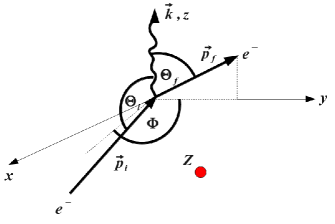
Figure 1: Parametrization of the Bremsstrahlung process: Momenta of incident electron $\mathbf{p}_{i}$, scattered electron $\mathbf{p}_{f}$ and emitted photon $\hbar\mathbf{k}$ form the angles $\Theta_{i}=\sphericalangle(\mathbf{p}_{i},\mathbf{k})$ and $\Theta_{f}=\sphericalangle(\mathbf{p}_{f},\mathbf{k})$, and $\Phi$ is the angle between the planes spanned by the vector pairs $(\mathbf{p}_{i},\mathbf{k})$ and $(\mathbf{p}_{f},\mathbf{k})$. The scattering nucleus has atomic number $Z$.

1.3 Available cross-sections for Bremsstrahlung

Our present understanding of Bremsstrahlung and pair production was largely developed in the first half of the 20th century. It was first calculated by Bethe and Heitler (1934). Important older reviews are by Heitler (1944), by Hough (1948), and by Koch and Motz (1959). We also used some recent text books (Greiner and Reinhardt, 1995; Peskin and Schroeder, 1995); together with Heitler (1944) and Hough (1948), they provide a good introduction into the quantum field theoretical description of Bremsstrahlung and pair production. The calculation of these two processes is related through some physical symmetry as will be explained in chapter 3.

As drawn in Fig. 1, when an electron scatters at a nucleus, a photon with frequency $\omega$ can be emitted. The geometry of this process is described by the three angles $\Theta_{i}$, $\Theta_{f}$ and $\Phi$. Cross sections can be total or differential. Total cross sections determine whether a collision takes place for given incident electron energy, singly differential cross sections give additional information on the photon energy or on the angle between incident electron and emitted photon, and doubly differential cross sections contain both. Triply differential cross sections additionally contain the angle at which the electron is scattered. As two angles are required to characterize the direction of the scattered electron, one could argue that this cross section should actually be called quadruply differential, but the standard terminology for the process is triply differential.

Koch and Motz (1959) review many different expressions for different limiting cases, but without derivations. Moreover, some experimental results are discussed and compared with the presented theory. Bethe and Heitler (1934), Heitler (1944), Hough (1948), Koch and Motz (1959), Peskin and Schroeder (1995), Greiner and Reinhardt (1955) use the Born approximation to derive and describe Bremsstrahlung and pair production cross sections.

Several years later new ansatzes were made to describe Bremsstrahlung. Elwert and Haug (1969) use approximate Sommerfeld-Maue eigenfunctions to derive cross sections for Bremsstrahlung under the assumption of a pure Coulomb field. They derive a triply differential cross section and beyond that also numerically a doubly differential cross section. Furthermore they compare with results obtained by using the Born approximation. They show that there is a small discrepancy for high atomic numbers between the Bethe-Heitler theory and experimental data, and they provide a correcting factor to fit the Bethe-Heitler approximation better to experimental data for large $Z$. However, they only investigate properties of Bremsstrahlung for $Z=13$ (aluminum) and $Z=79$ (gold).

Tseng and Pratt (1971) and Fink and Pratt (1973) use exact numerical calculations using Coulomb screened potentials and Furry-Sommerfeld-Maue wave functions, respectively. They investigate Bremsstrahlung and pair production for $Z=13$ and for $Z=79$ and show that their results with more accurate wave functions do not fit with the Bethe Heitler cross section exactly. This is not surprising as the Bethe-Heitler approximation is developed for low atomic numbers $Z$ and for $Z$ dependent electron energies as discussed in section 2.2.
Shaffer et al. (1996) review the Bethe Heitler and the Elwert Haug theory. They discuss that the Bethe Heitler approach is good for small atomic numbers and give a limit of $Z>29$ for experiments to deviate from theory. For $Z<29$ the theory of Bethe and Heitler, however, is stated to be in good agreement with experiments for energies above the keV range. They calculate triply differential cross sections using partial-wave and multipole expansions in a screened potential numerically for $Z=47$ (silver) and $Z=79$ and compare their results with experimental data. Actually their results are close to the Elwert Haug theory which fits the experimental data better than their theory.

Shaffer and Pratt (1997) also discuss the theory of Elwert and Haug (1969) and compare it with the Bethe Heitler theory and, additionally, with the Bethe Heitler results multiplied with the Elwert factor and with the exact partial wave method. They show that all theories agree within a factor 10 in the keV energy range, and that the Elwert-Haug theory fits the exact partial wave method best. However, they only investigate Bremsstrahlung for atomic nuclei with $Z=47$, 53 (iodine), 60 (neodymium), 68 (erbium) and 79, but not for small atomic numbers $Z=7$ and 8 as relevant in air. In summary, Elwert and Haug (1969), Tseng and Pratt (1971), Fink and Pratt (1973), Shaffer et al. (1996) and Shaffer and Pratt (1997) calculate cross sections for Bremsstrahlung and pair production for atomic numbers $Z=13$ and $Z>47$ numerically, but not analytically, and they do not provide any formula or data which can be used to simulate discharges in air.

The EEDL database consists mainly of experimental data which have been adjusted to nuclear model calculations. For the low energy range Geant4 takes over this data and gives a fit formula. The singly differential cross section related to $\omega$ which is used in the Geant4 toolkit is valid in an energy range from 1 keV to 10 GeV and taken from Seltzer and Berger (1985). The singly differential cross section related to $\Theta_{i}$ is based on the doubly differential cross section by (68; 69) and valid for very high energies, i.e., well above $(1-10)$ MeV. But in the preimplemented cross sections of Geant4 the dependence on the photon energy is neglected in this case so that it is actually a singly differential cross section describing $\Theta_{i}$.

Table 1 gives an overview of the available literature and data for total or singly, doubly or triply differential Bremsstrahlung cross sections; parameterized angles or photon energies are given, as well as the different energy ranges of the incident electron. Furthermore, the table shows the atomic number $Z$ investigated and includes some further remarks.

For calculating the angularly resolved photon energy spectrum of TGF’s, we need a doubly differential cross section resolving both energy and emission angle of the photons; we need it in the energy range between 1 keV and 1 GeV for the small atomic numbers $Z=7$ and 8. Therefore most of the literature reviewed here is not applicable. However, the Bethe-Heitler approximation is valid for atomic numbers $Z<29$ and for electron energies above 1 keV (58). How the range of validity depends on the atomic number $Z$ is discussed in section 2.2. We therefore will use the triply differential cross section derived by Bethe and Heitler (1934) to determine the correct doubly differential cross.

Data/Paper	Information	Energy range	Atomic Number $Z$	Remarks
Bethe and	$\omega$	1 keV - 1 GeV	7,8	energy range depends on $Z$
Heitler (1934,1944)	$\omega,\Theta_{i},\Theta_{f},\Phi$
	Total	different lower	depends on the
Koch and	$\omega$	bounds, no	used formulae
Motz (1959)	$\omega,\Theta_{i},\Phi$	upper bounds
	$\omega,\Theta_{i},\Theta_{f},\Phi$
Aiginger (1966)	$\omega,\Theta_{i}$	180, 380 keV	79, Al2O3	experimental
Elwert and	$\omega,\Theta_{i}$	keV range	13,79
Haug (1969)	$\omega,\Theta_{i},\Theta_{f},\Phi$
Penczynski and	$\omega,\Theta_{i}$	$(300\pm 10)$ keV	82	experimental
Wehner (1970)
Tseng and	$\omega,\Theta_{i},\Theta_{f},\Phi$	keV, MeV range	13,79
Pratt (1971)
Fink and	$\omega$	keV, MeV range	6,13,79,92	also for pair production
Pratt (1973)	$\omega,\Theta_{i},\Theta_{f},\Phi$
Tsai (1974,1977)	$\omega,\Theta_{i}$	$>$ few 10 MeV	all
Seltzer and	$\omega$	1 keV - 10 GeV	Z=6,13,29,47,74,92
Berger (1985)
EEDL (1991)	Total	5 eV - 1 TeV	all	see (12)
Nackel (1994)	$\omega,\Theta_{i}$	keV	6,29,47,79	only twodimensional description
Schaffer	$\omega,\Theta_{i},\Phi$	keV range	6,13,29,47,74,92
et al. (1996)
Schaffer and	$\omega,\Theta_{i},\Theta_{f},\Phi$	keV range	47,53,60,68,79
Pratt (1997)	$\omega,\Theta_{i}$
Lehtinen (2000)	$\omega,\Theta_{i}$	1 keV - 1 GeV	7,8	Simple product ansatz for
				angular and frequency part
	Total	5 eV - 1 TeV	all	based on EEDL
Geant 4 (2003)	$\omega$	1 keV - 10 GeV	6,13,29,47,74,92	based on Seltzer and Berger (1985)
	$\Theta_{i}$	$>$ few 10 MeV	all	based on Tsai (1974, 1977)

Table 1: Available data for Bremsstrahlung cross sections. Besides the available information on total or singly, doubly or triply differential cross-sections, the range of validity of the incident electron energy and of the atomic number is given. If not stated otherwise, these are theoretical expressions.

I

1.4 Bremsstrahlung data used by other TGF researchers

Carlson et al. (2009, 2010) use Geant 4, a library of sotware tools with a preimplemented database to simulate the production of Terrestrial Gamma-Ray Flashes. But Geant 4 does not supply an energy resolved angular distribution as it does not contain a doubly differential cross section, parameterizing both energy and emission angle of the Bremsstrahlung photons (see Table 1). Furthermore, it is designed for high electron energies. It also includes the Landau-Pomeranchuk-Migdal (LPM) (Landau and Pomeranchuk, 1953) effect and dielectric suppression (Ter-Mikaelian, 1954) which do not contribute in the keV and MeV range. We will briefly discuss the cross sections and effects implemented in Geant 4 in D.

Lehtinen has suggested a doubly differential cross section in his PhD thesis (Lehtlinen, 2000) that is also used by Xu et al. (2012). Lehtinen’s ansatz is a heuristic approach based on factorization into two factors. The first factor is the singly differential cross section of Bethe and Heitler (1934) that resolves only electron and photon energies, but no angles. The second factor is due to Jackson (1975, p. 712 et seq.), it depends on the variable $(1-\beta^{2})\;[(1-\beta\cos\Theta_{i})^{2}+(\cos\Theta_{i}-\beta)^{2}]\;/\;(1-\beta\cos\Theta_{i})^{4}$, where $\beta=|{\bf}v_{i}|/c$ measures the incident electron velocity on the relativistic scale. However, this factor derived in Jackson (1975, p. 712 et seq.) is calculated in the classical and not quantum mechanical case, and it is valid only if the photon energy is much smaller than the total energy of the incident electron. We will compare this ansatz with our results in E.

Dwyer (2007) chooses to use the triply differential cross section by Bethe and Heitler (1934), but with an additional form factor parameterizing the structure of the nucleus (36). We will show in F that this form factor, however, does not contribute for energies above 1 keV. This cross section depends on all three angles as shown in Fig. 1. If one is only interested in the angle $\Theta_{i}$ between incident electron and emitted Bremsstrahlung photon, the angles $\Theta_{f}$ and $\Phi$ have to be integrated out — either numerically, or the analytical results derived in the present paper can be used.

1.5 Organization of the paper

In chapter 2 we introduce the triply differential cross section derived by Bethe and Heitler Then we integrate over the two angles $\Theta_{f}$ and $\Phi$ to obtain the doubly differential cross section which gives a correlation between the energy of the emitted photon and its direction relative to the incident electron. Furthermore, we investigate the limit of very small or very large angles and of high photon energies; this also serves as a consistency check for the correct integration of the full expression.

In chapter 3 we perform the same calculations for pair production, i.e., when an incident photon interacts with an atomic nucleus and creates a positron electron pair. As we explain, this process is actually related by some physical symmetry to Bremsstrahlung, therefore results can be transferred from Bremsstrahlung to pair production. We get a doubly differential cross section for energy and emission angle of the created positron relative to direction and energy of the incident photon.

The physical interpretation and implications of our analytical results is discussed in chapter 4. Energies and emission angles of the created photons and positrons are described in the particular case of scattering on nitrogen nuclei. For electron energies below 100 keV, the emission of Bremsstrahlung photons in different directions varies typically by not more than an order of magnitude, while for higher electron energies the photons are mainly emitted in forward direction. For this case, we derive an analytical approximation for the most likely emission angle of Bremsstrahlung photons and positrons for given particle energies.

In chapter 5 we will briefly summarize the results of our calculations.

Details of our calculations can be found in A - I. Beyond that we provide a C++ code The C++ code can be downloaded directly from the website of the journal.

2 Bremsstrahlung

2.1 Definition of the process

If an electron with momentum $\mathbf{p}_{i}$ approaches the nucleus of an atom, it can change its direction due to Coulomb interaction with the nucleus; the electron acceleration creates a Bremsstrahlung photon with momentum $\mathbf{k}$ that can be emitted at an angle $\Theta_{i}$ relative to the initial direction of the electron. The new direction of the electron forms an angle $\Theta_{f}$ with the direction of the photon. The angle $\Phi$ is the angle between the planes spanned by the vector pairs $(\mathbf{p}_{i},\mathbf{k})$ and $(\mathbf{p}_{f},\mathbf{k})$. This process is shown in figure 1. A virtual photon (allowed by Heisenberg’s uncertainty principle) transfers a momentum ${\bf q}$ between the electron and the nucleus. Therefore both energy and momentum are conserved in the scattering process.

The corresponding triply differential cross section was derived by Bethe and Heitler (1934):

$$d^{4}\sigma = \frac{Z^{2}\alpha_{fine}^{3}\hbar^{2}}{(2\pi)^{2}}\frac{|\mathbf{p}_{f}|}{|\mathbf{p}_{i}|}\frac{d\omega}{\omega}\frac{d\Omega_{i}d\Omega_{f}d\Phi}{|\mathbf{q}|^{4}}\times$$ (1)

$$\times \left[\frac{\mathbf{p}_{f}^{2}\sin^{2}\Theta_{f}}{(E_{f}-c|\mathbf{p}_{f}|\cos\Theta_{f})^{2}}\left(4E_{i}^{2}-c^{2}\mathbf{q}^{2}\right)\right.$$

$$+ \frac{\mathbf{p}_{i}^{2}\sin^{2}\Theta_{i}}{(E_{i}-c|\mathbf{p}_{i}|\cos\Theta_{i})^{2}}\left(4E_{f}^{2}-c^{2}\mathbf{q}^{2}\right)$$

$$+ 2\hbar^{2}\omega^{2}\frac{\mathbf{p}_{i}^{2}\sin^{2}\Theta_{i}+\mathbf{p}_{f}^{2}\sin^{2}\Theta_{f}}{(E_{f}-c|\mathbf{p}_{f}|\cos\Theta_{f})(E_{i}-c|\mathbf{p}_{i}|\cos\Theta_{i})}$$

$$- 2\left.\frac{|\mathbf{p}_{i}||\mathbf{p}_{f}|\sin\Theta_{i}\sin\Theta_{f}\cos\Phi}{(E_{f}-c|\mathbf{p}_{f}|\cos\Theta_{f})(E_{i}-c|\mathbf{p}_{i}|\cos\Theta_{i})}\left(2E_{i}^{2}+2E_{f}^{2}-c^{2}\mathbf{q}^{2}\right)\right].$$

Here $Z$ is the atomic number of the nulceus, $\alpha_{fine}\approx{1}/{137}$ is the fine structure constant, $h\approx 6.63\cdot 10^{-34}$ Js is Planck’s constant, $\hbar=h/{2\pi}$ and $c\approx 3\cdot 10^{8}$ m/s is the speed of light. The kinetic energy $E_{kin,i/f}$ of the electron in the initial and final state is related to its total energy and momentum as

$$E_{i/f}=E_{kin,i/f}+m_{e}c^{2}=\sqrt{m_{e}^{2}c^{4}+\mathbf{p}_{i/f}^{2}c^{2}}$$ (2)

where $m_{e}\approx 9.1\cdot 10^{-31}$ kg is the electron mass. The conservation of energy implies

$$E_{f}=E_{i}-\hbar\omega$$ (3)

which determines $E_{f}$ as a function of $E_{i}$ and $\hbar\omega$. The directions of the emitted photon with energy $\hbar\omega$ and of the scattered electron are parameterized by the three angles (see Fig. 1)

$$\Theta_{i} = \sphericalangle(\mathbf{p}_{i},\mathbf{k}),$$ (4)

$$\Theta_{f} = \sphericalangle(\mathbf{p}_{f},\mathbf{k}),$$ (5)

$$\Phi = \textnormal{Angle between the planes $(\mathbf{p}_{i},\mathbf{k})$ and $(\mathbf{p}_{f},\mathbf{k})$}.$$ (6)

The differentials are

$$d\Omega_{i} = \sin\Theta_{i}\ d\Theta_{i},$$ (7)

$$d\Omega_{f} = \sin\Theta_{f}\ d\Theta_{f}.$$ (8)

Furthermore one can get an expression for the absolute value of the virtual photon $\mathbf{q}$ with the help of the momenta, the photon energy $\hbar\omega$ and the angles (4) - (6). Its value is

$$-\mathbf{q}^{2} = -|\mathbf{p}_{i}|^{2}-|\mathbf{p}_{f}|^{2}-\left(\frac{\hbar}{c}\omega\right)^{2}+2|\mathbf{p}_{i}|\frac{\hbar}{c}\omega\cos\Theta_{i}-2|\mathbf{p}_{f}|\frac{\hbar}{c}\omega\cos\Theta_{f}$$ (9)

$$+ 2|\mathbf{p}_{i}||\mathbf{p}_{f}|(\cos\Theta_{f}\cos\Theta_{i}+\sin\Theta_{f}\sin\Theta_{i}\cos\Phi).$$

2.2 Validity of the cross sections of Bethe and Heitler

The cross sections of Bethe and Heitler (1) are valid if the Born approximation (5) holds

$$v\gg\frac{Zc}{137}$$ (10)

For nitrogen with $Z=7$ and for oxygen with $Z=8$, this holds for electron velocities $|\mathbf{v}_{Z=7}|\gg 15\cdot 10^{6}$ m/s and $|\mathbf{v}_{Z=8}|\gg 18\cdot 10^{6}$ m/s; this is equivalent to a kinetic energy of

$$E_{kin}=\frac{m_{e}c^{2}}{\sqrt{1-\frac{v^{2}}{c^{2}}}}-m_{e}c^{2}\gg\left\{\begin{array}[]{c}670\ \textnormal{eV},\ Z=7\\ 875\ \textnormal{eV},\ Z=8\end{array}\right..$$ (13)

This means that incident electron energies above 1 keV can be treated with Eq. 1, for lower energies, one cannot calculate with free electron waves anymore, but has to use Coulomb waves (Heitler, 1944; Greiner und Reinhardt, 1995); in this case one cannot derive cross sections like (1) analytically any more. Thus the Bethe Heitler cross section and our results must not be used for energies of the electron in the initial and final state smaller than 1 keV. However, for higher energies of the electron in the initial and final state, the approximation by Bethe and Heitler becomes more accurate; thus this approximation is better if $E_{kin}\geq 10$ keV.

2.3 Integration over $\Phi$

The easiest way is to integrate over the angle $\Phi$ between the scattering planes first (see Fig. 1) . For this purpose it is useful to redefine some quantities in the following way; therefore (1) can be written much more simply:

$$\alpha := 2|\mathbf{p}_{i}||\mathbf{p}_{f}|\sin\Theta_{i}\sin\Theta_{f},$$ (14)

$$\beta := -\mathbf{p}_{i}^{2}-\mathbf{p}_{f}^{2}-\left(\frac{\hbar}{c}\omega\right)^{2}-2\frac{\hbar}{c}\omega|\mathbf{p}_{f}|\cos\Theta_{f}+2\frac{\hbar}{c}\omega|\mathbf{p}_{i}|\cos\Theta_{i}$$ (15)

$$+ 2|\mathbf{p}_{i}||\mathbf{p}_{f}|\cos\Theta_{i}\cos\Theta_{f}$$

$$A := \frac{Z^{2}\alpha_{fine}^{3}}{(2\pi)^{2}}\frac{|\mathbf{p}_{f}|}{|\mathbf{p}_{i}|}\frac{\hbar^{2}}{\omega},$$ (16)

$$a_{1} := \left(\frac{|\mathbf{p}_{f}|^{2}c^{2}\sin^{2}\Theta_{f}}{(E_{f}-|\mathbf{p}_{f}|c\cos\Theta_{f})^{2}}+\frac{|\mathbf{p}_{i}|^{2}c^{2}\sin^{2}\Theta_{i}}{(E_{i}-|\mathbf{p}_{i}|c\cos\Theta_{i})^{2}}\right)\cdot A,$$ (17)

$$a_{2} := \left(-\frac{2|\mathbf{p}_{i}||\mathbf{p}_{f}|c^{2}\sin\Theta_{i}\sin\Theta_{f}}{(E_{i}-|\mathbf{p}_{i}|c\cos\Theta_{i})(E_{f}-|\mathbf{p}_{f}|c\cos\Theta_{f})}\right)\cdot A,$$ (18)

$$a_{3} := \left(\frac{4E_{i}^{2}|\mathbf{p}_{f}|^{2}\sin^{2}\Theta_{f}}{(E_{f}-|\mathbf{p}_{f}|c\cos\Theta_{f})^{2}}+\frac{4E_{f}^{2}|\mathbf{p}_{i}|^{2}\sin^{2}\Theta_{i}}{(E_{i}-|\mathbf{p}_{i}|c\cos\Theta_{i})^{2}}\right.$$ (19)

$$+ \left.\frac{2\hbar^{2}\omega^{2}(|\mathbf{p}_{i}|^{2}\sin\Theta_{i}+|\mathbf{p}_{f}|^{2}\sin^{2}\Theta_{f})}{(E_{i}-|\mathbf{p}_{i}|c\cos\Theta_{i})(E_{f}-|\mathbf{p}_{f}|c\cos\Theta_{f})}\right)\cdot A,$$

$$a_{4} := \left(-\frac{|\mathbf{p}_{i}||\mathbf{p}_{f}|\sin\Theta_{i}\sin\Theta_{f}(4E_{i}^{2}+4E_{f}^{2})}{(E_{i}-|\mathbf{p}_{i}|c\cos\Theta_{i})(E_{f}-|\mathbf{p}_{f}|c\cos\Theta_{f})}\right)\cdot A.$$ (20)

With (14) - (20), Eq. (1) can be written as:

$$\frac{d^{4}\sigma}{d\omega\Omega_{i}d\Omega_{f}d\Phi} = \frac{a_{1}}{\alpha\cos\Phi+\beta}+\frac{a_{2}\cos\Phi}{\alpha\cos\Phi+\beta}$$ (21)

$$+ \frac{a_{3}}{(\alpha\cos\Phi+\beta)^{2}}+\frac{a_{4}\cos\Phi}{(\alpha\cos\Phi+\beta)^{2}};$$

thus the integration over $\Phi$ simply reads

$$\frac{d^{3}\sigma}{d\omega d\Omega_{i}d\Omega_{f}} = \int\limits_{0}^{2\pi}d\Phi\left[\frac{a_{1}}{\alpha\cos\Phi+\beta}+\frac{a_{2}\cos\Phi}{\alpha\cos\Phi+\beta}\right.$$ (22)

$$+ \left.\frac{a_{3}}{(\alpha\cos\Phi+\beta)^{2}}+\frac{a_{4}\cos\Phi}{(\alpha\cos\Phi+\beta)^{2}}\right]$$

where $a_{i},\ i\in\{1,\ldots,4\},\alpha$ and $\beta$ still depend on $\Theta_{f}$ and $\Theta_{i}$. These integrals can be calculated with the help of the residue theorem which is reviewed briefly in A. If $R(x,y):\mathbb{R}^{2}\rightarrow\mathbb{R}$ is a rational function without poles on the unit circle $x^{2}+y^{2}=1$, then

$$\int\limits_{0}^{2\pi}R(\cos\Phi,\sin\Phi)d\Phi=2\pi i\sum\limits_{|z|<1}\textnormal{Res}(f,z)$$ (23)

where $f$ is a complex function which is defined as

$$f(z):=\frac{1}{iz}R\left(\frac{1}{2}\left(z+\frac{1}{z}\right),\frac{1}{2i}\left(z-\frac{1}{z}\right)\right).$$ (24)

The residuum of a pole $z_{j}$ of order $n$ is defined as

$$\textnormal{Res}(f,z_{j})=\frac{1}{(n-1)!}\lim_{z\rightarrow z_{j}}\frac{d^{n-1}}{dz^{n-1}}\Big{[}(z-z_{j})f(z)\Big{]}.$$ (25)

To integrate the functions in Eq. (22), we write

$$R_{1}(x,y) := \frac{a_{1}}{\alpha x+\beta},$$ (26)

$$R_{2}(x,y) := \frac{a_{2}x}{\alpha x+\beta},$$ (27)

$$R_{3}(x,y) := \frac{a_{3}}{(\alpha x+\beta)^{2}},$$ (28)

$$R_{4}(x,y) := \frac{a_{4}x}{(\alpha x+\beta)^{2}};$$ (29)

and get from (24)

$$f_{1}(z) = \frac{2a_{1}}{i(\alpha z^{2}+2\beta z+\alpha)},$$ (30)

$$f_{2}(z) = \frac{a_{2}z^{2}+a_{2}}{zi(\alpha z^{2}+2\beta z+\alpha)},$$ (31)

$$f_{3}(z) = \frac{4a_{3}z}{i\left(\alpha z^{2}+2\beta z+\alpha\right)^{2}},$$ (32)

$$f_{4}(z) = \frac{2a_{4}(z^{2}+1)}{i\left(\alpha z^{2}+2\beta z+\alpha\right)^{2}}.$$ (33)

The poles of the functions $f_{i}(z)$ in (30) - (33) are given by

$$z_{1,2}=-\frac{\beta}{\alpha}\pm\sqrt{\left(\frac{\beta}{\alpha}\right)^{2}-1}.$$ (34)

For $f_{1,2}$ poles are of order one and for $f_{3,4}$ of order two. In addition $f_{2}$ has a pole at

$$z_{3}=0.$$ (35)

According to (23) one needs poles with $|z_{i}|<1$. For $z_{3}$ it is quite clear that $|z_{3}|=0<1$. As the angles $\Theta_{i}$ and $\Theta_{f}$ are between $0$ and $\pi$, the expression $\alpha>0$ in Eq. (14). Furthermore $\cos\Theta_{f}>-1$, $\cos\Theta_{i}<1$ and $|\mathbf{p_{i}}|>\hbar/c\ \omega$. Hence

$$\beta$$

$$= -\mathbf{p}_{i}^{2}-\mathbf{p}_{f}^{2}-\left(\frac{\hbar}{c}\omega\right)^{2}-2\frac{\hbar}{c}\omega|\mathbf{p}_{f}|\cos\Theta_{f}+2\frac{\hbar}{c}\omega|\mathbf{p}_{i}|\cos\Theta_{i}$$

$$+ 2|\mathbf{p}_{i}||\mathbf{p}_{f}|\cos\Theta_{i}\cos\Theta_{f}$$

$$= -\mathbf{p}_{i}^{2}-\mathbf{p}_{f}^{2}-\left(\frac{\hbar}{c}\omega\right)^{2}+2\frac{\hbar}{c}\omega|\mathbf{p}_{i}|\cos\Theta_{i}$$

$$+ 2|\mathbf{p}_{f}|\cos\Theta_{f}\left(-\frac{\hbar}{c}\omega+|\mathbf{p}_{i}|\cos\Theta_{i}\right)$$ (38)

$$< -\mathbf{p}_{i}^{2}-\mathbf{p}_{f}^{2}-\left(\frac{\hbar}{c}\omega\right)^{2}+2\frac{\hbar}{c}\omega|\mathbf{p}_{i}|+2|\mathbf{p}_{f}|\cos\Theta_{f}\left(-\frac{\hbar}{c}\omega+|\mathbf{p}_{i}|\right)$$ (39)

$$< -\mathbf{p}_{i}^{2}-\mathbf{p}_{f}^{2}-\left(\frac{\hbar}{c}\omega\right)^{2}+2\frac{\hbar}{c}\omega|\mathbf{p}_{i}|+2|\mathbf{p}_{f}|\left(-\frac{\hbar}{c}\omega+|\mathbf{p}_{i}|\right)$$ (40)

$$= -\mathbf{p}_{i}^{2}-\mathbf{p}_{f}^{2}-\left(\frac{\hbar}{c}\omega\right)^{2}+2\frac{\hbar}{c}\omega|\mathbf{p}_{i}|-2|\mathbf{p}_{f}|\frac{\hbar}{c}\omega+2|\mathbf{p}_{f}||\mathbf{p}_{i}|$$ (41)

$$= -\left(|\mathbf{p}_{i}|-|\mathbf{p}_{f}|-\frac{\hbar}{c}\omega\right)^{2}<0$$ (42)

Therefore $\beta/\alpha$ in Eq. (34) is a negative real number. Furthermore $\sin\Theta_{i}<1$ and $\sin\Theta_{f}<1$. Thus

$$-\beta-\alpha$$

$$= \mathbf{p}_{i}^{2}+\mathbf{p}_{f}^{2}+\left(\frac{\hbar}{c}\omega\right)^{2}+2\frac{\hbar}{c}\omega|\mathbf{p}_{f}|\cos\Theta_{f}-2\frac{\hbar}{c}\omega|\mathbf{p}_{i}|\cos\Theta_{i}$$

$$- 2|\mathbf{p}_{i}||\mathbf{p}_{f}|\cos\Theta_{i}\cos\Theta_{f}-2|\mathbf{p}_{i}||\mathbf{p}_{f}|\sin\Theta_{i}\sin\Theta_{f}$$ (44)

$$> \mathbf{p}_{i}^{2}+\mathbf{p}_{f}^{2}+\left(\frac{\hbar}{c}\omega\right)^{2}-2\frac{\hbar}{c}\omega|\mathbf{p}_{f}|-2\frac{\hbar}{c}\omega|\mathbf{p}_{i}|-4|\mathbf{p}_{i}||\mathbf{p}_{f}|$$ (45)

$$> \mathbf{p}_{i}^{2}+\mathbf{p}_{f}^{2}+\left(\frac{\hbar}{c}\omega\right)^{2}>0$$ (46)

$$\Rightarrow -\frac{\beta}{\alpha}>1$$ (47)

It follows immediately that $|z_{1}|>1$ and $|z_{2}|<1$. For all residua one obtains

$$\textnormal{Res}(f_{1},z_{2}) = -\frac{a_{1}}{i}\frac{1}{\sqrt{\beta^{2}-\alpha^{2}}},$$ (48)

$$\textnormal{Res}(f_{2},z_{2}) = \frac{a_{2}\beta}{\alpha i}\frac{1}{\sqrt{\beta^{2}-\alpha^{2}}},$$ (49)

$$\textnormal{Res}(f_{2},z_{3}) = \frac{a_{2}}{\alpha i},$$ (50)

$$\textnormal{Res}(f_{3},z_{2}) = -\frac{a_{3}\beta}{i}\frac{1}{(\sqrt{\beta^{2}-\alpha^{2}})^{3}},$$ (51)

$$\textnormal{Res}(f_{4},z_{2}) = a_{4}\alpha\frac{1}{(\sqrt{\beta^{2}-\alpha^{2}})^{3}}.$$ (52)

With the knowledge of these residua and using (23), the integral in (22) can be calculated elementarily

$$\frac{d^{3}\sigma}{d\omega d\Omega_{i}d\Omega_{f}}=\frac{2\pi a_{2}}{\alpha} + \frac{2\pi}{\sqrt{\beta^{2}-\alpha^{2}}}\left[-a_{1}+\frac{a_{2}\beta}{\alpha}\right.$$ (53)

$$- \left.\frac{a_{3}\beta}{|\beta^{2}-\alpha^{2}|}+\frac{a_{4}\alpha}{|\beta^{2}-\alpha^{2}|}\right].$$

2.4 Integration over $\Theta_{f}$

After having obtained an expression for the “triply” differential cross section, there is still the integration over $\Theta_{f}$ left. This calculation is mainly straight forward, but rather tedious. Using expression (53), it is

$$\frac{d^{2}\sigma}{d\omega d\Omega_{i}}=\int\limits_{0}^{\pi}d\Theta_{f}\left[\frac{2\pi a_{2}}{\alpha}\right. + \frac{2\pi}{\sqrt{\beta^{2}-\alpha^{2}}}\left(-a_{1}+\frac{a_{2}\beta}{\alpha}\right.$$ (54)

$$- \left.\left.\frac{a_{3}\beta}{|\beta^{2}-\alpha^{2}|}+\frac{a_{4}\alpha}{|\beta^{2}-\alpha^{2}|}\right)\right]\sin\Theta_{f}.$$

Let’s now consider the first integral of (54). If one inserts (14) and (18), it becomes

$$\int\limits_{0}^{\pi}d\Theta_{f}\frac{2\pi a_{2}}{\alpha}\sin\Theta_{f} = -\frac{2\pi Ac^{2}}{E_{i}-cp_{i}\cos\Theta_{i}}\int\limits_{0}^{\pi}d\Theta_{f}\frac{\sin\Theta_{f}}{E_{f}-cp_{f}\cos\Theta_{f}}$$ (55)

$$= -\frac{2\pi Ac^{2}}{E_{i}-cp_{i}\cos\Theta_{i}}\int\limits_{-1}^{+1}dx\frac{1}{E_{f}-cp_{f}x}$$ (56)

where the substitution $x:=\cos\Theta_{f}$ was made in the second step. (56) is rather simple and yields

$$\int\limits_{0}^{\pi}d\Theta_{f}\frac{2\pi a_{2}}{\alpha}\sin\Theta_{f}=-\frac{2\pi Ac}{(E_{i}-cp_{i}\cos\Theta_{i})p_{f}}\ln\left(\frac{E_{f}+p_{f}c}{E_{f}-p_{f}c}\right).$$ (57)

This was a quite simple calculation. All the other integrals can be calculated similarly, but with more effort. As another example let’s consider the last integral. Before inserting (14), (15) and (20) one can define for simplicity

$$\Delta_{1} := -\mathbf{p}_{i}^{2}-\mathbf{p}_{f}^{2}-\left(\frac{\hbar}{c}\omega\right)^{2}+2\frac{\hbar}{c}\omega|\mathbf{p}_{i}|\cos\Theta_{i},$$ (58)

$$\Delta_{2} := -2\frac{\hbar}{c}\omega|\mathbf{p}_{f}|+2|\mathbf{p}_{i}||\mathbf{p}_{f}|\cos\Theta_{i}.$$ (59)

The expression $\beta$ from Eq. (15) is then

$$\beta=\Delta_{1}+\Delta_{2}\cos\Theta_{f}.$$ (60)

Thus the regularly appearing term $\beta^{2}-\alpha^{2}$ can be written as

$$\beta^{2}-\alpha^{2} = (\Delta_{2}^{2}+4p_{i}^{2}p_{f}^{2}\sin^{2}\Theta_{i})\cos^{2}\Theta_{f}+2\Delta_{1}\Delta_{2}\cos\Theta_{f}$$ (61)

$$+ (\Delta_{1}^{2}-4p_{i}^{2}p_{f}^{2}\sin^{2}\Theta_{i})$$

$$= \Box_{1}^{2}\cos^{2}\Theta_{f}+2\Delta_{1}\Delta_{2}\cos\Theta_{f}+\Box_{2}^{2}$$ (62)

where the definitions

$$\Box_{1}^{2} := \Delta_{2}^{2}+4p_{i}^{2}p_{f}^{2}\sin^{2}\Theta_{i},$$ (63)

$$\Box_{2}^{2} := \Delta_{1}^{2}-4p_{i}^{2}p_{f}^{2}\sin^{2}\Theta_{i}$$ (64)

have been introduced.

By using (14), (20) and (62), the last integral of (53) becomes

$$\int\limits_{0}^{\pi}d\Theta_{f}\frac{2\pi a_{4}\alpha}{\sqrt{(\beta^{2}-\alpha^{2})^{3}}}\sin\Theta_{f}=-\frac{16\pi Ap_{i}^{2}p_{f}^{2}\sin^{2}\Theta_{i}(E_{i}^{2}+E_{f}^{2})}{E_{i}-cp_{i}\cos\Theta_{i}}$$ (66)

$$\times \int\limits_{0}^{\pi}d\Theta_{f}\frac{\sin^{2}\Theta_{f}}{\sqrt{(\Box_{1}^{2}\cos\Theta_{f}^{2}+2\Delta_{1}\Delta_{2}\cos\Theta_{f}+\Box_{2}^{2})^{3}}(E_{f}-cp_{f}\cos\Theta_{f})}\sin\Theta_{f}$$

$$= -\frac{16\pi Ap_{i}^{2}p_{f}^{2}\sin^{2}\Theta_{i}(E_{i}^{2}+E_{f}^{2})}{E_{i}-cp_{i}\cos\Theta_{i}}$$

$$\times \int\limits_{-1}^{+1}dx\frac{1-x^{2}}{\sqrt{(\Box_{1}^{2}x^{2}+2\Delta_{1}\Delta_{2}x+\Box_{2}^{2})^{3}}(E_{f}-cp_{f}x)}$$

where $x=\cos\Theta_{f}$ has been substituted again.
This integration can be performed elementarily by finding the indefinite integral

$$\frac{\Box_{1}^{2}x^{2}+2\Delta_{1}\Delta_{2}x+\Box_{2}^{2}}{\sqrt{(\Box_{1}^{2}x^{2}+2\Delta_{1}\Delta_{2}x+\Box_{2}^{2})^{3}}(\Delta_{1}^{2}\Delta_{2}^{2}-\Box_{1}^{2}\Box_{2}^{2})(\Box_{1}^{2}E_{f}^{2}+2\Delta_{1}\Delta_{2}E_{f}p_{f}c+\Box_{2}^{2}p_{f}c)}\times$$ (67)

$$\times \left(-\Box_{1}^{4}E_{f}x+\Box_{2}^{4}p_{f}c+2\Delta_{1}^{2}\Delta_{2}^{2}(E_{f}x-p_{f}c)+\Delta_{1}\Delta_{2}\Box_{2}^{2}(E_{f}+p_{f}cx)\right.$$

$$- \left.\Box_{1}^{2}(\Box_{2}^{2}(E_{f}x-p_{f}c)\Delta_{1}\Delta_{2}(E_{f}+p_{f}cx))\right)$$

$$+ \frac{E_{f}^{2}-p_{f}^{2}c^{2}}{\sqrt{(\Box_{1}^{2}E_{f}^{2}+2\Delta_{1}\Delta_{2}E_{f}p_{f}c+\Box_{2}^{2}p_{f}c)^{3}}}\ln\Bigl{(}(E_{f}-p_{f}cx)(\Box_{1}^{2}E_{f}x+\Box_{2}^{2}p_{f}c$$

$$+ \Delta_{1}\Delta_{2}(E_{f}+p_{f}cx)+\sqrt{\Box_{1}^{2}x^{2}+2\Delta_{1}\Delta_{2}x+\Box_{2}^{2}}\times$$

$$\times \sqrt{\Box_{1}^{2}E_{f}^{2}+2\Delta_{1}\Delta_{2}E_{f}p_{f}c+\Box_{2}^{2}p_{f}c})\Bigr{)},$$

by inserting $+1$ and $-1$ as upper and lower limit, using (63) and (64) and simplifying. The integral in (LABEL:theta.12) is then finally

$$\int\limits_{0}^{\pi}d\Theta_{f}\frac{2\pi a_{4}\alpha}{\sqrt{(\beta^{2}-\alpha^{2})^{3}}}\sin\Theta_{f} - \frac{16\pi Ap_{i}^{2}p_{f}^{2}\sin^{2}\Theta_{i}(E_{i}^{2}+E_{f}^{2})}{E_{i}-cp_{i}\cos\Theta_{i}}\times$$

$$\times \left[-\frac{2(\Delta_{2}p_{f}c+\Delta_{1}E_{f})}{(-\Delta_{2}^{2}+\Delta_{1}^{2}-4p_{i}^{2}p_{f}^{2}\sin^{2}\Theta_{i})((\Delta_{2}E_{f}+\Delta_{1}p_{f}c)^{2}+4m^{2}c^{4}p_{i}^{2}p_{f}^{2}\sin^{2}\Theta_{i})}\right.$$

$$+ \frac{m^{2}c^{4}}{\sqrt{((\Delta_{2}E_{f}+\Delta_{1}p_{f}c)^{2}+4m^{2}c^{4}p_{i}^{2}p_{f}^{2}\sin^{2}\Theta_{i})^{3}}}\times$$

$$\times \ln\Bigg{(}\Big{(}(E_{f}-cp_{f})(4p_{i}^{2}p_{f}^{2}\sin^{2}\Theta_{i}(-E_{f}-p_{f}c)+(\Delta_{1}-\Delta_{2})((\Delta_{2}E_{f}+\Delta_{1}p_{f}c)$$

$$- \sqrt{\Box_{1}^{2}E_{f}^{2}+2\Delta_{1}\Delta_{2}E_{f}p_{f}c+\Box_{2}^{2}p_{f}c})\Big{)}\Big{(}(E_{f}+cp_{f})(4p_{i}^{2}p_{f}^{2}\sin^{2}\Theta_{i}(+E_{f}-p_{f}c)$$

$$+ (\Delta_{1}+\Delta_{2})((\Delta_{2}E_{f}+\Delta_{1}p_{f}c)-\sqrt{\Box_{1}^{2}E_{f}^{2}+2\Delta_{1}\Delta_{2}E_{f}p_{f}c+\Box_{2}^{2}p_{f}c})\Big{)}^{-1}\Bigg{)}\Bigg{]}.$$

All the other integrals can be calculated similarly where one always has to substitute $x=\cos\Theta_{f}$. With this technique the whole doubly differential cross section finally becomes

$$\frac{d^{2}\sigma(E_{i},\omega,\Theta_{i})}{d\omega d\Omega_{i}}=\sum\limits_{j=1}^{6}I_{j}$$ (69)

with the following contributions:

$$I_{1} = \frac{2\pi A}{\sqrt{\Delta_{2}^{2}+4p_{i}^{2}p_{f}^{2}\sin^{2}\Theta_{i}}}\ln\left(\frac{\Delta_{2}^{2}+4p_{i}^{2}p_{f}^{2}\sin^{2}\Theta_{i}-\sqrt{\Delta_{2}^{2}+4p_{i}^{2}p_{f}^{2}\sin^{2}\Theta_{i}}(\Delta_{1}+\Delta_{2})+\Delta_{1}\Delta_{2}}{-\Delta_{2}^{2}-4p_{i}^{2}p_{f}^{2}\sin^{2}\Theta_{i}-\sqrt{\Delta_{2}^{2}+4p_{i}^{2}p_{f}^{2}\sin^{2}\Theta_{i}}(\Delta_{1}-\Delta_{2})+\Delta_{1}\Delta_{2}}\right)$$ (70)

$$\times \left[1+\frac{c\Delta_{2}}{p_{f}(E_{i}-cp_{i}\cos\Theta_{i})}-\frac{p_{i}^{2}c^{2}\sin^{2}\Theta_{i}}{(E_{i}-cp_{i}\cos\Theta_{i})^{2}}-\frac{2\hbar^{2}\omega^{2}p_{f}\Delta_{2}}{c(E_{i}-cp_{i}\cos\Theta_{i})(\Delta_{2}^{2}+4p_{i}^{2}p_{f}^{2}\sin^{2}\Theta_{i})}\right],$$

$$I_{2} = -\frac{2\pi Ac}{p_{f}(E_{i}-cp_{i}\cos\Theta_{i})}\ln\left(\frac{E_{f}+p_{f}c}{E_{f}-p_{f}c}\right),$$ (71)

$$I_{3} = \frac{2\pi A}{\sqrt{(\Delta_{2}E_{f}+\Delta_{1}p_{f}c)^{2}+4m^{2}c^{4}p_{i}^{2}p_{f}^{2}\sin^{2}\Theta_{i}}}$$

$$\times \ln\Bigg{(}\Big{(}(E_{f}+p_{f}c)(4p_{i}^{2}p_{f}^{2}\sin^{2}\Theta_{i}(E_{f}-p_{f}c)+(\Delta_{1}+\Delta_{2})((\Delta_{2}E_{f}+\Delta_{1}p_{f}c)$$

$$- \sqrt{(\Delta_{2}E_{f}+\Delta_{1}p_{f}c)^{2}+4m^{2}c^{4}p_{i}^{2}p_{f}^{2}\sin^{2}\Theta_{i}}))\Big{)}\Big{(}(E_{f}-p_{f}c)(4p_{i}^{2}p_{f}^{2}\sin^{2}\Theta_{i}(-E_{f}-p_{f}c)$$

$$+ (\Delta_{1}-\Delta_{2})((\Delta_{2}E_{f}+\Delta_{1}p_{f}c)-\sqrt{(\Delta_{2}E_{f}+\Delta_{1}p_{f}c)^{2}+4m^{2}c^{4}p_{i}^{2}p_{f}^{2}\sin^{2}\Theta_{i}}))\Big{)}^{-1}\Bigg{)}$$

$$\times \left[-\frac{(\Delta_{2}^{2}+4p_{i}^{2}p_{f}^{2}\sin^{2}\Theta_{i})(E_{f}^{3}+E_{f}p_{f}^{2}c^{2})+p_{f}c(2(\Delta_{1}^{2}-4p_{i}^{2}p_{f}^{2}\sin^{2}\Theta_{i})E_{f}p_{f}c+\Delta_{1}\Delta_{2}(3E_{f}^{2}+p_{f}^{2}c^{2}))}{(\Delta_{2}E_{f}+\Delta_{1}p_{f}c)^{2}+4m^{2}c^{4}p_{i}^{2}p_{f}^{2}\sin^{2}\Theta_{i}}\right.$$

$$- \frac{c(\Delta_{2}E_{f}+\Delta_{1}p_{f}c)}{p_{f}(E_{i}-cp_{i}\cos\Theta_{i})}$$

$$- \frac{4E_{i}^{2}p_{f}^{2}(2(\Delta_{2}E_{f}+\Delta_{1}p_{f}c)^{2}-4m^{2}c^{4}p_{i}^{2}p_{f}^{2}\sin^{2}\Theta_{i})(\Delta_{1}E_{f}+\Delta_{2}p_{f}c)}{((\Delta_{2}E_{f}+\Delta_{1}p_{f}c)^{2}+4m^{2}c^{4}p_{i}^{2}p_{f}^{2}\sin^{2}\Theta_{i})^{2}}$$

$$+ \left.\frac{8p_{i}^{2}p_{f}^{2}m^{2}c^{4}\sin^{2}\Theta_{i}(E_{i}^{2}+E_{f}^{2})-2\hbar^{2}\omega^{2}p_{i}^{2}\sin^{2}\Theta_{i}p_{f}c(\Delta_{2}E_{f}+\Delta_{1}p_{f}c)+2\hbar^{2}\omega^{2}p_{f}m^{2}c^{3}(\Delta_{2}E_{f}+\Delta_{1}p_{f}c)}{(E_{i}-cp_{i}\cos\Theta_{i})((\Delta_{2}E_{f}+\Delta_{1}p_{f}c)^{2}+4m^{2}c^{4}p_{i}^{2}p_{f}^{2}\sin^{2}\Theta_{i})}\right],$$

$$I_{4} = -\frac{4\pi Ap_{f}c(\Delta_{2}E_{f}+\Delta_{1}p_{f}c)}{(\Delta_{2}E_{f}+\Delta_{1}p_{f}c)^{2}+4m^{2}c^{4}p_{i}^{2}p_{f}^{2}\sin^{2}\Theta_{i}}-\frac{16\pi E_{i}^{2}p_{f}^{2}A(\Delta_{2}E_{f}+\Delta_{1}p_{f}c)^{2}}{((\Delta_{2}E_{f}+\Delta_{1}p_{f}c)^{2}+4m^{2}c^{4}p_{i}^{2}p_{f}^{2}\sin^{2}\Theta_{i})^{2}},$$ (73)

$$I_{5} = \frac{4\pi A}{(-\Delta_{2}^{2}+\Delta_{1}^{2}-4p_{i}^{2}p_{f}^{2}\sin^{2}\Theta_{i})((\Delta_{2}E_{f}+\Delta_{1}p_{f}c)^{2}+4m^{2}c^{4}p_{i}^{2}p_{f}^{2}\sin^{2}\Theta_{i})}$$ (74)

$$\times \left[\frac{\hbar^{2}\omega^{2}p_{f}^{2}}{E_{i}-cp_{i}\cos\Theta_{i}}\right.$$

$$\times \frac{E_{f}[2\Delta_{2}^{2}(\Delta_{2}^{2}-\Delta_{1}^{2})+8p_{i}^{2}p_{f}^{2}\sin^{2}\Theta_{i}(\Delta_{2}^{2}+\Delta_{1}^{2})]+p_{f}c[2\Delta_{1}\Delta_{2}(\Delta_{2}^{2}-\Delta_{1}^{2})-16\Delta_{1}\Delta_{2}p_{i}^{2}p_{f}^{2}\sin^{2}\Theta_{i}]}{\Delta_{2}^{2}+4p_{i}^{2}p_{f}^{2}\sin^{2}\Theta_{i}}$$

$$+ \frac{2\hbar^{2}\omega^{2}p_{i}^{2}\sin^{2}\Theta_{i}(2\Delta_{1}\Delta_{2}p_{f}c+2\Delta_{2}^{2}E_{f}+8p_{i}^{2}p_{f}^{2}\sin^{2}\Theta_{i}E_{f})}{E_{i}-cp_{i}\cos\Theta_{i}}$$

$$+ \frac{2E_{i}^{2}p_{f}^{2}\{2(\Delta_{2}^{2}-\Delta_{1}^{2})(\Delta_{2}E_{f}+\Delta_{1}p_{f}c)^{2}+8p_{i}^{2}p_{f}^{2}\sin^{2}\Theta_{i}[(\Delta_{1}^{2}+\Delta_{2}^{2})(E_{f}^{2}+p_{f}^{2}c^{2})+4\Delta_{1}\Delta_{2}E_{f}p_{f}c]\}}{((\Delta_{2}E_{f}+\Delta_{1}p_{f}c)^{2}+4m^{2}c^{4}p_{i}^{2}p_{f}^{2}\sin^{2}\Theta_{i})}$$

$$+ \left.\frac{8p_{i}^{2}p_{f}^{2}\sin^{2}\Theta_{i}(E_{i}^{2}+E_{f}^{2})(\Delta_{2}p_{f}c+\Delta_{1}E_{f})}{E_{i}-cp_{i}\cos\Theta_{i}}\right],$$

$$I_{6} = \frac{16\pi E_{f}^{2}p_{i}^{2}\sin^{2}\Theta_{i}A}{(E_{i}-cp_{i}\cos\Theta_{i})^{2}(-\Delta_{2}^{2}+\Delta_{1}^{2}-4p_{i}^{2}p_{f}^{2}\sin^{2}\Theta_{i})}.$$ (75)

Eq. (69) depends explicitly on $E_{i},\omega$ and $\Theta_{i}$ while $E_{f}$ and $p_{f}$ are functions of $E_{i}$ and $\omega$ through (2) and (3). (69) is the final result of the integration of (1) over $\Phi$ and $\Theta_{f}$ with the help of the residue theorem and some basic calculations. Now this result can be used both as input for Monte Carlo code and for discussing some basic properties of the behaviour of produced Bremsstrahlung photons.
Actually (69) is also valid for $\Theta_{i}=0$, as will be shown in the next section, but the simple way just to set $\Theta_{i}=0$ in (69) will fail, especially for numerical purposes, because the logarithmic part in (70) tends to $\ln(0/0)$ for $\Theta_{i}\rightarrow 0$ and so fails for numerical applications. Thus we need an additional expression for $\Theta_{i}=0$ which has to be consistent with (69).

2.5 Special limits: $\Theta_{i}=0,\pi$ and $\hbar\omega\rightarrow E_{kin,i}$

For some special cases the integration of (1) over $\Phi$ and $\Theta_{f}$ is easier. This information can also be used to verify (69) by checking consistency and use them for Monte Carlo codes.

2.5.1 $\Theta_{i}=0$ or $\Theta_{i}=\pi$

If one is only interested in forward and backward scattering, one can set $\Theta_{i}=0$ or $\Theta_{i}=\pi$ before integrating; then (1) becomes

$$\frac{d^{4}\sigma}{d\omega d\Omega_{i}d\Omega_{f}d\Phi} = \frac{Z^{2}\alpha_{fine}^{3}\hbar^{2}}{(2\pi)^{2}}\frac{|\mathbf{p}_{f}|}{|\mathbf{p}_{i}|}\frac{1}{\omega}\frac{1}{|\mathbf{q}|^{4}}$$ (76)

$$\times \left(\frac{\mathbf{p}_{f}^{2}\sin^{2}\Theta_{f}}{(E_{f}-c|\mathbf{p}_{f}|\cos\Theta_{f})^{2}}\left(4E_{i}^{2}-c^{2}\mathbf{q}^{2}\right)\right.$$

$$+ 2\left.\hbar^{2}\omega^{2}\frac{\mathbf{p}_{f}^{2}\sin^{2}\Theta_{f}}{(E_{f}-c|\mathbf{p}_{f}|\cos\Theta_{f})(E_{i}\mp c|\mathbf{p}_{i}|\cos\Theta_{i})}\right)$$

where the momentum $\mathbf{q}$ of the virtual photon can be written as

$$-\mathbf{q}^{2}=-\mathbf{p}_{i}^{2}-\mathbf{p}_{f}^{2}-\left(\frac{\hbar}{c}\omega\right)^{2}-2\frac{\hbar}{c}|\mathbf{p}_{f}|\cos\Theta_{f}\pm 2\frac{\hbar}{c}\omega|\mathbf{p}_{i}|\pm 2|\mathbf{p}_{i}||\mathbf{p}_{f}|\cos\Theta_{f}.$$

(77)

Here the upper sign corresponds to $\Theta_{i}=0$ and the lower one to $\Theta_{i}=\pi$.
As (76) and (77) do not depend on $\Phi$ at all, the $\Phi$ integration simply gives a factor of $2\pi$, and (76) becomes

$$\frac{d^{3}\sigma}{d\omega d\Omega_{i}d\Omega_{f}} = \frac{Z^{2}\alpha_{fine}^{3}\hbar^{2}}{2\pi}\frac{|\mathbf{p}_{f}|}{|\mathbf{p}_{i}|}\frac{1}{\omega}\frac{1}{|\mathbf{q}|^{4}}$$ (78)

$$\times \left(\frac{\mathbf{p}_{f}^{2}\sin^{2}\Theta_{f}}{(E_{f}-c|\mathbf{p}_{f}|\cos\Theta_{f})^{2}}\left(4E_{i}^{2}-c^{2}\mathbf{q}^{2}\right)\right.$$

$$+ 2\left.\hbar^{2}\omega^{2}\frac{\mathbf{p}_{f}^{2}\sin^{2}\Theta_{f}}{(E_{f}-c|\mathbf{p}_{f}|\cos\Theta_{f})(E_{i}\mp c|\mathbf{p}_{i}|\cos\Theta_{i})}\right).$$

Finally this expression has to be integrated over $\Theta_{f}$ in order to obtain the doubly differential cross section. Similarly to the total integration of (54) it is convenient to define

$$\tilde{\Delta}_{1} := -\left(p_{i}\mp\frac{\hbar}{c}\omega\right)^{2}-p_{f}^{2},$$ (79)

$$\tilde{\Delta}_{2} := -2\frac{\hbar}{c}\omega p_{f}\pm 2p_{i}p_{f}$$ (80)

where $\tilde{\Delta}_{1,2}=\Delta_{1,2}(\Theta_{i}=0,\pi),j\in\{1,2\}$ , with definitions (58) and (59). Eq. (77) can then be rewritten as

$$-\mathbf{q}^{2}=\tilde{\Delta}_{1}+\tilde{\Delta}_{2}\cos\Theta_{f}$$ (81)

and

$$\frac{d^{2}\sigma}{d\omega d\Omega_{i}} = \frac{Z^{2}\alpha_{fine}^{3}\hbar^{2}}{2\pi}\frac{|\mathbf{p}_{f}|}{|\mathbf{p}_{i}|}\frac{1}{\omega}\int\limits_{0}^{\pi}d\Theta_{f}\left[\frac{|\mathbf{p}_{f}|^{2}c^{2}\sin^{2}\Theta_{f}}{(E_{f}-|\mathbf{p}_{f}|c\cos\Theta_{f})^{2}(\tilde{\Delta}_{1}+\tilde{\Delta}_{2}\cos\Theta_{f})}\right.$$

$$+ \frac{4E_{i}^{2}|\mathbf{p}_{f}|^{2}\sin^{2}\Theta_{f}}{(E_{f}-|\mathbf{p}_{f}|c\cos\Theta_{f})^{2}(\tilde{\Delta}_{1}+\tilde{\Delta}_{2}\cos\Theta_{f})^{2}}$$

$$+ \left.\frac{2\hbar^{2}\omega^{2}|\mathbf{p}_{f}|^{2}\sin^{2}\Theta_{f}}{(E_{i}\mp c|\mathbf{p}_{i}|)(E_{f}-|\mathbf{p}_{f}|c\cos\Theta_{f})(\tilde{\Delta}_{1}+\tilde{\Delta}_{2}\cos\Theta_{f})^{2}}\right]\sin\Theta_{f}$$

where the integration is rather elementary and can be performed by substituting $x=\cos\Theta_{f}$ again. Thus (LABEL:small.7) yields

$$\frac{d^{2}\sigma}{d\omega d\Omega_{i}}(E_{i},\omega,\Theta_{i}=0,\pi)=\frac{Z^{2}\alpha^{3}\hbar^{2}}{2\pi}\frac{|\mathbf{p}_{f}|}{|\mathbf{p}_{i}|}\frac{1}{\omega}\left[-\frac{2|\mathbf{p}_{f}|c}{\tilde{\Delta}_{2}E_{f}+\tilde{\Delta}_{1}|\mathbf{p}_{f}|c}\right.$$ (83)

$$+ \frac{|\mathbf{p}_{f}|^{2}c^{2}(-\tilde{\Delta}_{1}^{2}+\tilde{\Delta}_{2}^{2})}{\tilde{\Delta}_{2}(\tilde{\Delta}_{2}E_{f}+\tilde{\Delta}_{1}|\mathbf{p}_{f}|c)^{2}}\ln\left(\frac{\tilde{\Delta}_{1}+\tilde{\Delta}_{2}}{\tilde{\Delta}_{1}-\tilde{\Delta}_{2}}\right)$$

$$+ \frac{2\tilde{\Delta}_{1}E_{f}|\mathbf{p}_{f}|c+\tilde{\Delta}_{2}(E_{f}^{2}+|\mathbf{p}_{f}|^{2}c^{2})}{(\tilde{\Delta}_{2}E_{f}+\tilde{\Delta}_{1}|\mathbf{p}_{f}|c)^{2}}\ln\left(\frac{E_{f}+|\mathbf{p}_{f}|c}{E_{f}-|\mathbf{p}_{f}|c}\right)$$

$$- \frac{16E_{i}^{2}|\mathbf{p}_{f}|^{2}}{(\tilde{\Delta}_{2}E_{f}+\tilde{\Delta}_{1}|\mathbf{p}_{f}|c)^{2}}-\frac{4\hbar^{2}|\mathbf{p}_{f}|^{2}\omega^{2}}{(\tilde{\Delta}_{2}E_{f}+\tilde{\Delta}_{1}|\mathbf{p}_{f}|c)(E_{i}\mp c|\mathbf{p}_{i}|)\tilde{\Delta}_{2}}$$

$$- \frac{8E_{i}^{2}|\mathbf{p}_{f}|^{2}(\tilde{\Delta}_{1}E_{f}+\tilde{\Delta}_{2}|\mathbf{p}_{f}|c)}{(\tilde{\Delta}_{2}E_{f}+\tilde{\Delta}_{1}|\mathbf{p}_{f}|c)^{3}}\ln\left(\frac{(\tilde{\Delta}_{1}-\tilde{\Delta}_{2})(E_{f}-|\mathbf{p}_{f}|c)}{(\tilde{\Delta}_{1}+\tilde{\Delta}_{2})(E_{f}+|\mathbf{p}_{f}|c)}\right)$$

$$+ \frac{2\hbar^{2}|\mathbf{p}_{f}|^{2}\omega^{2}(2\tilde{\Delta}_{1}\tilde{\Delta}_{2}E_{f}+\tilde{\Delta}_{1}^{2}|\mathbf{p}_{f}|c+\tilde{\Delta}_{2}^{2}|\mathbf{p}_{f}|c)}{(\tilde{\Delta}_{2}E_{f}+\tilde{\Delta}_{1}|\mathbf{p}_{f}|c)^{2}(E_{i}\mp c|\mathbf{p}_{i}|)\tilde{\Delta}_{2}^{2}}\ln\left(\frac{\tilde{\Delta}_{1}+\tilde{\Delta}_{2}}{\tilde{\Delta}_{1}-\tilde{\Delta}_{2}}\right)$$

$$+ \left.\frac{2\hbar^{2}|\mathbf{p}_{f}|\omega^{2}(E_{f}^{2}-c^{2}|\mathbf{p}_{f}|^{2})}{(\tilde{\Delta}_{2}E_{f}+\tilde{\Delta}_{1}|\mathbf{p}_{f}|c)^{2}(E_{i}\mp c|\mathbf{p}_{i}|)c}\ln\left(\frac{E_{f}-|\mathbf{p}_{f}|c}{E_{f}+|\mathbf{p}_{f}|c}\right)\right].$$

This expression is much simpler than (69), but only valid for $\Theta_{i}=0$ or $\Theta_{i}=\pi$. Actually this expression has also been obtained by calculating the limit $\Theta_{i}\rightarrow 0$ or $\Theta_{i}\rightarrow\pi$ in (69); hence the consistency check is succesful. Details can be found in B.

2.5.2 $\hbar\omega\rightarrow E_{kin,i}$

The other case which can be investigated easily is when almost all kinetic energy of the incident electron is transferred to the emitted photon, i.e.,

$$E_{f}=E_{i}-\hbar\omega=E_{kin,i}+m_{e}c^{2}-\hbar\omega\xrightarrow{\hbar\omega\rightarrow E_{kin,i}}m_{e}c^{2}$$ (84)

and

$$|\mathbf{p}_{f}|=\sqrt{\frac{E_{f}^{2}}{c^{2}}-m_{e}^{2}c^{2}}\xrightarrow{\hbar\omega\rightarrow E_{kin,i}}\sqrt{\frac{m_{e}^{2}c^{4}}{c^{2}}-m_{e}^{2}c^{2}}\equiv 0$$ (85)

and consequently from Eq. (9)

$$-\mathbf{q}^{2}\xrightarrow{\hbar\omega\rightarrow E_{kin,i}}-\mathbf{p}_{i}^{2}-\left(\frac{\hbar}{c}\omega\right)^{2}+2\frac{\hbar}{c}\omega|\mathbf{p}_{i}|\cos\Theta_{i} =: \delta$$ (86)

$$\Rightarrow\mathbf{q}^{4} \xrightarrow{\hbar\omega\rightarrow E_{kin,i}} \delta^{2}.$$ (87)

With these limits it follows for the triply differential cross section (1)

$$\frac{d^{4}\sigma}{d\omega d\Omega_{i}d\Omega_{f}d\Phi} \xrightarrow{\hbar\omega\rightarrow E_{kin,i}} \frac{Z^{2}\alpha_{fine}^{3}\hbar^{2}}{(2\pi)^{2}}\frac{|\mathbf{p}_{f}|}{|\mathbf{p}_{i}|}\frac{1}{\omega}\frac{1}{\delta^{2}}\left[\frac{|\mathbf{p}_{i}|^{2}\sin^{2}\Theta_{i}}{(E_{i}-c|\mathbf{p}_{i}|\cos\Theta_{i})^{2}}\right.$$

$$\times (4E_{f}^{2}+\delta c^{2})+2\left.\hbar^{2}\omega^{2}\frac{|\mathbf{p}_{i}|^{2}\sin^{2}\Theta_{i}}{(E_{i}-c|\mathbf{p}_{i}|\cos\Theta_{i})E_{f}}\right].$$

Actually (LABEL:limit.5) depends neither on $\Phi$, nor on $\Theta_{f}$. Therefore

$$\int\limits_{0}^{2\pi}d\Phi\int\limits_{0}^{\pi}\sin\Theta_{i}d\Theta_{i}=4\pi$$ (89)

which leads to a very simple expression for the doubly differential cross section

$$\frac{d^{2}\sigma}{d\omega d\Omega_{i}}\xrightarrow{\hbar\omega\rightarrow E_{kin,i}} \frac{Z^{2}\alpha^{3}\hbar^{2}}{\pi}\frac{|\mathbf{p}_{f}|}{|\mathbf{p}_{i}|}\frac{1}{\omega}\frac{1}{\delta^{2}}\left[\frac{|\mathbf{p}_{i}|^{2}\sin^{2}\Theta_{i}}{(E_{i}-c|\mathbf{p}_{i}|\cos\Theta_{i})^{2}}(4E_{f}^{2}+\delta c^{2})\right.$$ (90)

$$+ 2\left.\hbar^{2}\omega^{2}\frac{|\mathbf{p}_{i}|^{2}\sin^{2}\Theta_{i}}{(E_{i}-c|\mathbf{p}_{i}|\cos\Theta_{i})E_{f}}\right].$$

Although taking the limit $\hbar\omega\rightarrow E_{kin,i}$ contradicts Eq. (13) as the energy of the emitted electron should be larger than $1$ keV (13), (90) can be used for two purposes.
As (90) can be obtained, as well, by taking the limit $|\mathbf{p}_{f}|\rightarrow 0$ in (69), the complicated expression (69) is checked for consistency analytically. For further details the reader is referred to C. Furthermore we will see in section 4.1.5 that the most probable scattering angle does not depend on the photon energy for $E_{kin,i}\geq 1$ MeV. Therefore this cross section can be used for calculating the most probable scattering angle in this energy range.

3 Pair production

Pairs of electrons and positrons can be produced if a photon interacts with the nucleus of an atom. This process is related by some symmetry to the production of Bremsstrahlung photons. Bremsstrahlung occurs when an electron is affected by the nucleus of an atom, scattered and then emits a photon. So there are three real particles involved: incident electron, scattered electron and emitted photon. As the photon has no antiparticle one can change the time direction of the photon. For antimatter it is well known that antiparticles can be interpreted as the corresponding particles moving back in time. So one can substitute the incident electron by an positron moving forward in time. Thus by substituting emitted photon by incident photon and incident electron by emitted positron (due to time reversal and changing its charge) it is possible to describe pair production from Bremsstrahlung. Thus the emitted photon in the Bremsstrahlung process has to be substituted by the incident photon from the nucleus and the incident electron by the produced positron. With these two replacements one gets the differential cross section for pair production (32; 28)

$$d^{4}\sigma = \frac{Z^{2}\alpha_{fine}^{3}c^{2}}{(2\pi)^{2}\hbar}|\mathbf{p}_{+}||\mathbf{p}_{-}|\frac{dE_{+}}{\omega^{3}}\frac{d\Omega_{+}d\Omega_{-}d\Phi}{|\mathbf{q}|^{4}}\times$$

$$\times \left[-\frac{\mathbf{p}_{-}^{2}\sin^{2}\Theta_{-}}{(E_{-}-c|\mathbf{p}_{-}|\cos\Theta_{-})^{2}}\left(4E_{+}^{2}-c^{2}\mathbf{q}^{2}\right)\right.$$

$$- \frac{\mathbf{p}_{+}^{2}\sin^{2}\Theta_{+}}{(E_{+}-c|\mathbf{p}_{+}|\cos\Theta_{+})^{2}}\left(4E_{-}^{2}-c^{2}\mathbf{q}^{2}\right)$$

$$+ 2\hbar^{2}\omega^{2}\frac{\mathbf{p}_{+}^{2}\sin^{2}\Theta_{+}+\mathbf{p}_{-}^{2}\sin^{2}\Theta_{-}}{(E_{+}-c|\mathbf{p}_{+}|\cos\Theta_{+})(E_{-}-c|\mathbf{p}_{-}|\cos\Theta_{-})}$$

$$+ 2\left.\frac{|\mathbf{p}_{+}||\mathbf{p}_{-}|\sin\Theta_{+}\sin\Theta_{-}\cos\Phi}{(E_{+}-c|\mathbf{p}_{+}|\cos\Theta_{+})(E_{-}-c|\mathbf{p}_{-}|\cos\Theta_{-})}\left(2E_{+}^{2}+2E_{-}^{2}-c^{2}\mathbf{q}^{2}\right)\right],$$

where $Z$, $\alpha_{fine}$, $h$, $\hbar$ and $c$ are the same parameters as in Eq. (1). $\omega$ is the frequency of the incident photon, $E_{\pm}$ and $p_{\pm}$ are the total energy and the momentum of the positron/electron with

$$E_{\pm}=\sqrt{\mathbf{p}_{\pm}^{2}c^{2}+m_{e}^{2}c^{4}}.$$ (92)

Similarly to (1) there are three angles, $\Theta_{\pm}$ between the direction of the photon and the positron/electron direction, $\Theta_{+}=\sphericalangle(\mathbf{p}_{+},\mathbf{k}),\Theta_{-}=\sphericalangle(\mathbf{p}_{-},\mathbf{k})$, and $\Phi$ is the angle between the scattering planes $(\mathbf{p}_{+},\mathbf{k})$ and $(\mathbf{p}_{-},\mathbf{k})$. The absolute value of the momentum of the virtual photon is

$$-\mathbf{q}^{2} = -|\mathbf{p}_{+}|^{2}-|\mathbf{p}_{-}|^{2}-\left(\frac{\hbar}{c}\omega\right)^{2}+2|\mathbf{p}_{+}|\frac{\hbar}{c}\omega\cos\Theta_{+}+2|\mathbf{p}_{-}|\frac{\hbar}{c}\omega\cos\Theta_{-}$$ (93)

$$- 2|\mathbf{p}_{+}||\mathbf{p}_{-}|(\cos\Theta_{+}\cos\Theta_{-}+\sin\Theta_{+}\sin\Theta_{-}\cos\Phi).$$

Algebraically one obtains (LABEL:pair.1) from (1) by replacing

$$E_{f} \rightarrow E_{-},$$ (94)

$$E_{i} \rightarrow -E_{+},$$ (95)

$$\mathbf{p}_{i} \rightarrow -\mathbf{p}_{+},$$ (96)

$$\mathbf{p}_{f} \rightarrow \mathbf{p}_{-},$$ (97)

$$\omega \rightarrow -\omega,$$ (98)

$$\Theta_{i} \rightarrow \pi-\Theta_{+},$$ (99)

$$\Theta_{f} \rightarrow \Theta_{-},$$ (100)

$$\Phi \rightarrow \Phi-\pi$$ (101)

where the quantities on the left hand side are for Bremsstrahlung, and those on the right hand side for pair production. At the end one has to multiply with an additional factor to get the correct prefactor. With all the mentioned substitutions it is

$$d^{4}\sigma_{brems} \leftarrow \frac{\hbar^{3}\omega^{2}}{|\mathbf{p}_{+}|^{2}c^{2}}\frac{d\omega}{dE_{+}}d^{4}\sigma_{pair},$$ (102)

Because of this symmetry the results for pair production follow easily from those for Bremsstrahlung.
The direction of the positron relative to the incident photon is given by integrating (LABEL:pair.1) over $\Phi$ and $\Theta_{-}$. But this is the same exercise as to integrate (1) over $\Phi$ and $\Theta_{f}$. Because of the symmetry between Bremsstrahlung and pair production one can take (69) and substitute (94) - (101) to obtain a doubly differential cross section

$$\frac{d^{2}\sigma(E_{+},\omega,\Theta_{+})}{dE_{+}d\Omega_{+}}=\sum\limits_{j=1}^{6}I_{j}$$ (103)

with the following contributions

$$I_{1} = \frac{2\pi A}{\sqrt{(\Delta^{(p)}_{2})^{2}+4p_{+}^{2}p_{-}^{2}\sin^{2}\Theta_{i}}}$$

$$\times \ln\left(\frac{(\Delta^{(p)}_{2})^{2}+4p_{+}^{2}p_{-}^{2}\sin^{2}\Theta_{i}-\sqrt{(\Delta^{(p)}_{2})^{2}+4p_{+}^{2}p_{-}^{2}\sin^{2}\Theta_{i}}(\Delta^{(p)}_{1}+\Delta^{(p)}_{2})+\Delta^{(p)}_{1}\Delta^{(p)}_{2}}{-(\Delta^{(p)}_{2})^{2}-4p_{+}^{2}p_{-}^{2}\sin^{2}\Theta_{i}-\sqrt{(\Delta^{(p)}_{2})^{2}+4p_{+}^{2}p_{-}^{2}\sin^{2}\Theta_{i}}(\Delta^{(p)}_{1}-\Delta^{(p)}_{2})+\Delta^{(p)}_{1}\Delta^{(p)}_{2}}\right)$$

$$\times \left[-1-\frac{c\Delta^{(p)}_{2}}{p_{-}(E_{+}-cp_{+}\cos\Theta_{i})}+\frac{p_{+}^{2}c^{2}\sin^{2}\Theta_{i}}{(E_{+}-cp_{+}\cos\Theta_{i})^{2}}-\frac{2\hbar^{2}\omega^{2}p_{-}\Delta^{(p)}_{2}}{c(E_{+}-cp_{+}\cos\Theta_{i})((\Delta^{(p)}_{2})^{2}+4p_{+}^{2}p_{-}^{2}\sin^{2}\Theta_{i})}\right],$$

$$I_{2} = \frac{2\pi Ac}{p_{-}(E_{+}-cp_{+}\cos\Theta_{i})}\ln\left(\frac{E_{-}+p_{-}c}{E_{-}-p_{-}c}\right),$$ (105)

$$I_{3} = \frac{2\pi A}{\sqrt{(\Delta^{(p)}_{2}E_{-}+\Delta^{(p)}_{1}p_{-}c)^{2}+4m^{2}c^{4}p_{+}^{2}p_{-}^{2}\sin^{2}\Theta_{i}}}$$ (106)

$$\times \ln\Bigg{(}\Big{(}(E_{-}+p_{-}c)(4p_{+}^{2}p_{-}^{2}\sin^{2}\Theta_{i}(E_{-}-p_{-}c)+(\Delta^{(p)}_{1}+\Delta^{(p)}_{2})((\Delta^{(p)}_{2}E_{-}+\Delta^{(p)}_{1}p_{-}c)$$

$$- \sqrt{(\Delta^{(p)}_{2}E_{-}+\Delta^{(p)}_{1}p_{-}c)^{2}+4m^{2}c^{4}p_{+}^{2}p_{-}^{2}\sin^{2}\Theta_{i}}))\Big{)}\Big{(}(E_{-}-p_{-}c)(4p_{+}^{2}p_{-}^{2}\sin^{2}\Theta_{i}(-E_{-}-p_{-}c)$$

$$+ (\Delta^{(p)}_{1}-\Delta^{(p)}_{2})((\Delta^{(p)}_{2}E_{-}+\Delta^{(p)}_{1}p_{-}c)-\sqrt{(\Delta^{(p)}_{2}E_{-}+\Delta^{(p)}_{1}p_{-}c)^{2}+4m^{2}c^{4}p_{+}^{2}p_{-}^{2}\sin^{2}\Theta_{i}}))\Big{)}^{-1}\Bigg{)}$$

$$\times \left[\frac{c(\Delta^{(p)}_{2}E_{-}+\Delta^{(p)}_{1}p_{-}c)}{p_{-}(E_{+}-cp_{+}\cos\Theta_{i})}\right.$$

$$+ \Big{[}((\Delta^{(p)}_{2})^{2}+4p_{+}^{2}p_{-}^{2}\sin^{2}\Theta_{i})(E_{-}^{3}+E_{-}p_{-}c)+p_{-}c(2((\Delta^{(p)}_{1})^{2}-4p_{+}^{2}p_{-}^{2}\sin^{2}\Theta_{i})E_{-}p_{-}c$$

$$+ \Delta^{(p)}_{1}\Delta^{(p)}_{2}(3E_{-}^{2}+p_{-}^{2}c^{2}))\Big{]}\Big{[}(\Delta^{(p)}_{2}E_{-}+\Delta^{(p)}_{1}p_{-}c)^{2}+4m^{2}c^{4}p_{+}^{2}p_{-}^{2}\sin^{2}\Theta_{i}\Big{]}^{-1}$$

$$+ \Big{[}-8p_{+}^{2}p_{-}^{2}m^{2}c^{4}\sin^{2}\Theta_{i}(E_{+}^{2}+E_{-}^{2})-2\hbar^{2}\omega^{2}p_{+}^{2}\sin^{2}\Theta_{i}p_{-}c(\Delta^{(p)}_{2}E_{-}+\Delta^{(p)}_{1}p_{-}c)$$

$$+ 2\hbar^{2}\omega^{2}p_{-}m^{2}c^{3}(\Delta^{(p)}_{2}E_{-}+\Delta^{(p)}_{1}p_{-}c)\Big{]}\Big{[}(E_{+}-cp_{+}\cos\Theta_{i})((\Delta^{(p)}_{2}E_{-}+\Delta^{(p)}_{1}p_{-}c)^{2}+4m^{2}c^{4}p_{+}^{2}p_{-}^{2}\sin^{2}\Theta_{i})\Big{]}^{-1}$$

$$+ \left.\frac{4E_{+}^{2}p_{-}^{2}(2(\Delta^{(p)}_{2}E_{-}+\Delta^{(p)}_{1}p_{-}c)^{2}-4m^{2}c^{4}p_{+}^{2}p_{-}^{2}\sin^{2}\Theta_{i})(\Delta^{(p)}_{1}E_{-}+\Delta^{(p)}_{2}p_{-}c)}{((\Delta^{(p)}_{2}E_{-}+\Delta^{(p)}_{1}p_{-}c)^{2}+4m^{2}c^{4}p_{+}^{2}p_{-}^{2}\sin^{2}\Theta_{i})^{2}}\right],$$

$$I_{4} = \frac{4\pi Ap_{-}c(\Delta^{(p)}_{2}E_{-}+\Delta^{(p)}_{1}p_{-}c)}{(\Delta^{(p)}_{2}E_{-}+\Delta^{(p)}_{1}p_{-}c)^{2}+4m^{2}c^{4}p_{+}^{2}p_{-}^{2}\sin^{2}\Theta_{i}}+\frac{16\pi E_{+}^{2}p_{-}^{2}A(\Delta^{(p)}_{2}E_{-}+\Delta^{(p)}_{1}p_{-}c)^{2}}{((\Delta^{(p)}_{2}E_{-}+\Delta^{(p)}_{1}p_{-}c)^{2}+4m^{2}c^{4}p_{+}^{2}p_{-}^{2}\sin^{2}\Theta_{i})^{2}},$$ (107)

$$I_{5} = \frac{4\pi A}{(-(\Delta^{(p)}_{2})^{2}+(\Delta^{(p)}_{1})^{2}-4p_{+}^{2}p_{-}^{2}\sin^{2}\Theta_{i})((\Delta^{(p)}_{2}E_{-}+\Delta^{(p)}_{1}p_{-}c)^{2}+4m^{2}c^{4}p_{+}^{2}p_{-}^{2}\sin^{2}\Theta_{i})}$$ (108)

$$\times \left[\frac{\hbar^{2}\omega^{2}p_{-}^{2}}{E_{+}cp_{+}\cos\Theta_{i}}\Big{[}E_{-}[2(\Delta^{(p)}_{2})^{2}((\Delta^{(p)}_{2})^{2}-(\Delta^{(p)}_{1})^{2})+8p_{+}^{2}p_{-}^{2}\sin^{2}\Theta_{i}((\Delta^{(p)}_{2})^{2}+(\Delta^{(p)}_{1})^{2})]\right.$$

$$+ p_{-}c[2\Delta^{(p)}_{1}\Delta^{(p)}_{2}((\Delta^{(p)}_{2})^{2}-(\Delta^{(p)}_{1})^{2})-16\Delta^{(p)}_{1}\Delta^{(p)}_{2}p_{+}^{2}p_{-}^{2}\sin^{2}\Theta_{i}]\Big{]}\Big{[}(\Delta^{(p)}_{2})^{2}+4p_{+}^{2}p_{-}^{2}\sin^{2}\Theta_{i}\Big{]}^{-1}$$

$$+ \frac{2\hbar^{2}\omega^{2}p_{+}^{2}\sin^{2}\Theta_{i}(2\Delta^{(p)}_{1}\Delta^{(p)}_{2}p_{-}c+2(\Delta^{(p)}_{2})^{2}E_{-}+8p_{+}^{2}p_{-}^{2}\sin^{2}\Theta_{i}E_{-})}{E_{+}-cp_{+}\cos\Theta_{i}}$$

$$- \Big{[}2E_{+}^{2}p_{-}^{2}\{2((\Delta^{(p)}_{2})^{2}-(\Delta^{(p)}_{1})^{2})(\Delta^{(p)}_{2}E_{-}+\Delta^{(p)}_{1}p_{-}c)^{2}+8p_{+}^{2}p_{-}^{2}\sin^{2}\Theta_{i}[((\Delta^{(p)}_{1})^{2}+(\Delta^{(p)}_{2})^{2})(E_{-}^{2}+p_{-}^{2}c^{2})$$

$$+ 4\Delta^{(p)}_{1}\Delta^{(p)}_{2}E_{-}p_{-}c]\}\Big{]}\Big{[}(\Delta^{(p)}_{2}E_{-}+\Delta^{(p)}_{1}p_{-}c)^{2}+4m^{2}c^{4}p_{+}^{2}p_{-}^{2}\sin^{2}\Theta_{i}\Big{]}^{-1}$$

$$- \left.\frac{8p_{+}^{2}p_{-}^{2}\sin^{2}\Theta_{i}(E_{+}^{2}+E_{-}^{2})(\Delta^{(p)}_{2}p_{-}c+\Delta^{(p)}_{1}E_{-})}{E_{+}-cp_{+}\cos\Theta_{i}}\right],$$

$$I_{6} = -\frac{16\pi E_{-}^{2}p_{+}^{2}\sin^{2}\Theta_{i}A}{(E_{+}-cp_{+}\cos\Theta_{i})^{2}(-(\Delta^{(p)}_{2})^{2}+(\Delta^{(p)}_{1})^{2}-4p_{+}^{2}p_{-}^{2}\sin^{2}\Theta_{+})}$$ (109)

with

$$A=\frac{Z^{2}\alpha_{fine}^{3}c^{2}}{(2\pi)^{2}\hbar}\frac{|\mathbf{p}_{+}||\mathbf{p}_{-}|}{\omega^{3}},$$ (110)

and with $\Delta^{(p)}_{1},\Delta^{(p)}_{2}$ defined as

$$\Delta^{(p)}_{1} := -|\mathbf{p}_{+}|^{2}-|\mathbf{p}_{-}|^{2}-\left(\frac{\hbar}{c}\omega\right)+2\frac{\hbar}{c}\omega|\mathbf{p}_{+}|\cos\Theta_{+},$$ (111)

$$\Delta^{(p)}_{2} := 2\frac{\hbar}{c}\omega|\mathbf{p}_{i}|-2|\mathbf{p}_{+}||\mathbf{p}_{-}|\cos\Theta_{+}.$$ (112)

4 Discussion

4.1 Bremsstrahlung

4.1.1 Comparison with experiments

If electrons are scattered at nuclei, they can produce hard Bremsstrahlung photons with frequency $\omega$ and direction $\Theta_{i}$ relative to the direction of the electrons.
Figure 2 compares our equation (69) with experimental results for

a) $E_{kin,i}=180$ keV, $\hbar\omega=50$ keV           b) $E_{kin,i}=380$ keV, $\hbar\omega=100$ keV

Figure 2: $\omega/Z^{2}\cdot d^{2}\sigma/{(d\omega d\Omega_{i})}(E_{kin,i},\omega,\Theta_{i})$ for Bremsstrahlung as a function of the scattering angle $\Theta_{i}$ between emitted photon and incident electron for gold $Z=79$ where 1 mb = $10^{-31}$ m². The energies are a) $E_{kin,i}=180$ keV, $\hbar\omega=50$ keV and b) $E_{kin,i}=380$ keV, $\hbar\omega=100$ keV. The solid lines shows our result (69); the dotted lines show experimental values (Aiginiger, 1966).

gold ($Z=79$) for different electron and photon energies (Aiginger, 1966). For $Z=79$ the minimal electron energy (13) for the Born approximation to be valid, is $E_{kin,\{i,f\}}=115$ keV. Figure 2 shows that the cross sections agree overall in size for $E_{kin,i}=180$ keV, $\hbar\omega=50$ keV and for $E_{kin,i}=380$ keV, $\hbar\omega=100$ keV. However, for the first case, the energy of the electron in the final state is $E_{kin,f}=130$ keV $\approx 115$ keV, thus close to the velocity limit. Therefore there is a larger deviation, especially for small angles, than for the second case where a very good agreement can be observed.

4.1.2 Angular distribution of Bremsstrahlung

Figure 3 shows the doubly differential cross section (69) for Bremsstrahlung for several electron and photon energies.

a) $E_{kin,i}=10$ keV                                   b) $E_{kin,i}=150$ keV

c) $E_{kin,i}=1$ MeV                                   d) $E_{kin,i}=100$ MeV

Figure 3: The doubly differential cross section $d^{2}\sigma/{(d\omega d\Omega_{i})}(E_{kin,i},\omega,\Theta_{i})$ for Bremsstrahlung ($Z=7$) versus the scattering angle $\Theta_{i}$ between emitted photon and incident electron. The electron energies are a) $E_{kin,i}=10$ keV, b) $E_{kin,i}=150$ keV, c) $E_{kin,i}=1$ MeV and d) $E_{kin,i}=100$ MeV. In each plot the the photon energy $\hbar\omega$ amounts to $1\%,10\%,50\%$ and $95\%$ of the kinetic energy of the incident electron.

At first, the probability for generating photons decreases with increasing photon energy for fixed electron energy. This can be understood easily by applying (90). As can be seen there, the doubly differential cross section grows linearly in the momentum of the electron in the final state which is equivalent to

$$\frac{d^{2}\sigma}{d\omega d\Omega_{i}}\sim|\mathbf{p}_{f}|$$ (113)

for high photon energies. So, if all kinetic energy is transferred from the electron onto the photon, the final momentum $|\mathbf{p}_{f}|$ vanishes, and thus

$$\frac{d^{2}\sigma}{d\omega d\Omega_{i}}\rightarrow 0.$$ (114)

For nonrelativistic electron and photon energies the scattering angle tends to be mainly equally distributed, i.e. the photons do not have a preference for a particular direction. When the photon energy increases, photons are mainly emitted in forward direction, but the ratio between forward and backward scattering is at least three orders of magnitude lower than for a relativistic electron. This case belongs to the classical case where the velocity is small compared to the speed of light. Namely, it is $v/c|_{E_{kin,i}=10\textnormal{keV}}\approx 0.20$ and non-relativistic equations will be enough to describe these phenomena. In the relativistic case ($v/c|_{E_{kin,i}=1\textnormal{MeV}}\approx 0.94$ and $v/c|_{E_{kin,i}=100\textnormal{MeV}}\approx 0.99999$) the differential cross section becomes more and more anisotropic. Forward scattering is preferred to backward scattering although the maximal cross section does not lie precisely at $\Theta_{i}=0$ as can be seen in figure 3 c). But the more the electron energy increases the more the maximum wanders to smaller angles, for example, it seems in figure 3 d) that the maximal emission is indeed for $\Theta_{i}$=0. As mentioned in section 2.4 and in B, formula (70) cannot be evaluated directly at $\Theta_{i}=0$. However, for this purpose, we derived (83) which is valid for $\Theta_{i}=0$ and $\Theta_{i}=\pi$.

a) $E_{kin,i}=1$ MeV                                   b) $E_{kin,i}=100$ MeV

Figure 4: The doubly differential cross section $d^{2}\sigma/(d\omega d\Omega_{i})$ as in figure 3 for a smaller angular range

a)                                                          b)

Figure 5: The ratio between the doubly differential cross section for backward scattering ($\Theta_{i}=180^{\circ}$) $d^{2}\sigma(E_{kin,i},\omega,\Theta_{i}=180^{\circ})/(d\omega d\Omega_{i})$ and the maximum of this cross section $\max\left(d^{2}\sigma(E_{kin,i},\omega,\Theta_{i})/(d\omega d\Omega_{i})\right)$ vs. the kinetic energy of the incident electron for different ratios between photon and electron energies in a a) linear and b) logarithmic scale for $Z=7$ .

Figure 4 shows again (69) for two relativistic electron and different photon energies but for a smaller range of angles. It shows in more detail that the angle of maximal scattering is small, but not 0.
Figure 5 shows the ratio between the cross section for backward scattering and forward scattering. It can be clearly seen that the tendency for backward scattering decreases for increasing electron energy. The lower the electron energy becomes, the more forward and backward scattering become similar and in general, the scattering tends to be isotropic. Only for ratios between photon energies and electron energies close to 1, forward scattering is preferred for the whole range of energies, but still decreases with increasing electron energies.
In energetic electron avalanches electrons scatter frequently which leads to a large velocity dispersion. It depends on the direction of the applied electric field whether electrons move forward or whether their directions are distributed arbitrarily. If so, however, this implies that photons will not necessarily move in a preferred direction, but in the direction of the incident electron. Their motion and thus change of direction depend on photon processes, such as Compton scattering.

4.1.3 Relativistic transformation

The tendency of forward scattering in the case of relativistic incident electrons can be understood by applying the laws of relativistic transformations. Imagine a non-quantum field theoretical description of Bremsstrahlung  (35). If one regards an inertial system in which the incident particle is at rest (Fig. 6 a) ), radiation is emitted isotropically with a small-angle deflection.

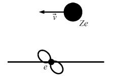
a) b)

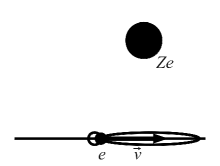
Figure 6: a) In the rest frame of the electron where the nucleus is moving instead radiation is emitted isotropically with a small-angle deflection. b) If, however, one transforms the situation into the rest frame of the nucleus where the electron is moving, most of the radiation is emitted in forward direction relative to the direction of the electron.

If the physical laws for this process are relativistically transformed into the laboratory system where the nucleus is at rest and the electron moving, most of the radiation is emitted in forward direction relative to the electron direction (Fig. 6 b) ). Because this transformation is valid for a non-quantum field theoretical, relativistic electron, it must also be true for a relativistic quantum theoretical description, therefore we see that the forward scattering of photons can simply be explained as a result of the relativistic transformation.

a) $E_{kin,i}=400$ keV                                   b) $E_{kin,i}=m_{e}c^{2}\approx 511$ keV

Figure 7: The doubly differential cross section $d^{2}\sigma/{(d\omega d\Omega_{i})}(E_{kin,i},\omega,\Theta_{i})$ for Bremsstrahlung ($Z=7$) versus the scattering angle $\Theta_{i}$ between emitted photon and incident electron. The electron energies are a) $E_{kin,i}=400$ keV, b) $E_{kin,i}\approx 511$ keV. In each plot the the photon energy $\hbar\omega$ amounts to $1\%,10\%,50\%$ and $95\%$ of the kinetic energy of the incident electron.

The forward scattering can moreover be understood by using the conservation laws of energy and momentum. They predict that photons have to be scattered in forward direction if electron and photon energy are high. The interested reader is referred to H.
Although figure 3 shows that the maxima of the doubly differential cross section form with increasing electron energy, it is difficult to determine in these plots when these maxima really start to be generated clearly. Figure 7 shows the doubly differential cross section in dependence of the incident electron energy for $E_{kin,i}=400$ keV and $E_{kin,i}\approx 511$ keV when the kinetic energy is equal to the rest energy. For $400$ keV and for $\hbar\omega/E_{kin,i}=0.01$ the cross section for forward scattering is already two orders of magnitude larger than for backward scattering, but a clear maximum cannot be seen. However, for the same kinetic energy, but for $\hbar\omega/E_{kin,i}=0.95$ there is already a clear maximum formed. But if the kinetic energy grows up to $511$ keV which is equal to the rest energy of the electron, there is even a maximum for $\hbar\omega=0.01E_{kin,i}$. This can be expected due to the relativistic transformation. If $E_{kin,i}\ll m_{e}c^{2}$, then the photon emission is relatively isotropic. But if the kinetic energy is approximately equal to the rest energy of the electron, relativistic laws are valid. Especially for $E_{kin,i}=m_{e}c^{2}$

$$\frac{v}{c}=\frac{\sqrt{3}}{2}\approx 87\%,$$ (115)

therefore the electron has to be treated relativistically and clear maxima close to $\Theta_{i}=0$ form for every possible photon energy.

4.1.4 Dependence on the energy of the emitted photon

Figure 3 shows that for both slow and relativistic electrons the doubly differentical cross section also varies with the photon energy for fixed electron energies. For fixed electron energy, lower photon energies are more likely. Moreover, photons are more likely for certain angles. They are more likely for lowly energetic electrons in the limit $\Theta_{i}\rightarrow 180^{\circ}$ and for highly energetic electrons in the limit $\Theta_{i}\rightarrow 0^{\circ}$. Figure 8 shows the doubly differential cross section in another way. Now the photon energy is fixed and the electron energy differs within one plot. For all cases it is more likely that low energetic electrons create photons than relativistic electrons do, in the limit $\Theta_{i}\rightarrow 180^{\circ}$. But for small angles, i.e. for forward emission of photons, the probability rapidly increases for relativistic electrons and exceeds the probability at small electron energies.

a) $\hbar\omega=50$ eV                                   b) $\hbar\omega=500$ eV

c) $\hbar\omega=500$ keV                                   d) $\hbar\omega=950$ keV

Figure 8: The doubly differential cross section $d^{2}\sigma/{(d\omega d\Omega_{i})}(E_{kin,i},\omega,\Theta_{i})$ for Bremsstrahlung ($Z=7$) vs. the scattering angle $\Theta_{i}$ for several electron and photon energies. In each panel the photon energy $\hbar\omega$ is fixed and the cross section is plotted for various kinetic energies of the incident electron.

4.1.5 The most probable scattering angle

Figure 3 also shows that the angle for which maximal scattering takes place, is rather independent of the photon energy. Hence, one can use (90) to determine a formula for that scattering angle. Actually this derivation leads to a quartic equation which can, however, be approximated for small angles, i.e. $\Theta_{i}\lesssim 20^{\circ}$, through a quadratic equation. The reader is referred to I for the detailed calculation. The solution of the quadratic equation reads

$$\Theta_{i}=\sqrt{\frac{-\frac{\delta_{0}}{\hbar\omega}(4E_{f}^{2}+\delta_{0}c^{2})-\frac{2\delta_{0}\hbar\omega}{E_{f}}(E_{i}-c|\mathbf{p}_{i}|)}{2\frac{|\mathbf{p}_{i}|}{c}\left[4E_{f}^{2}+\delta_{0}c^{2}+\frac{2\hbar^{2}\omega^{2}}{E_{f}}(E_{i}-c|\mathbf{p}_{i}|)\right]-|\mathbf{p}_{i}|\delta_{0}c-\frac{\hbar\omega}{E_{f}}c|\mathbf{p}_{i}|\delta_{0}}}$$ (116)

with

$$\delta_{0}:=-|\mathbf{p}_{i}|^{2}-\left(\frac{\hbar}{c}\omega\right)^{2}+2\frac{\hbar}{c}\omega|\mathbf{p}_{i}|,$$ (117)

$\hbar\omega\rightarrow E_{kin,i}$, e.g. $\hbar\omega=0.9999E_{kin,i}$ and

$$p_{i}=\sqrt{E_{kin,i}\left(\frac{E_{kin,i}}{c^{2}}+2m_{e}\right)}.$$ (118)

a)                                                          b)

Figure 9: $\Theta_{i}$ for maximal scattering vs. incident electron energy in a a) semilog and b) loglog plot for $Z=7$ . Besides (116) for $\hbar\omega=0.9999E_{kin,i}$, the exact solution of the quartic equation and various data for different $\hbar\omega/E_{kin,i}$ are shown.

Figure 9 shows (116) and manually extracted values for $\Theta_{i}$ for different photon energies. It shows much better than figure 3 that $\Theta_{i}$ is rather independent of the photon energy for relativistic electron energies. Besides (116), the solution of the quartic equation, is shown. Moreover, it shows that (116) gives a good approximation for those angles $\Theta_{i}$ for which scattering is maximal. Actually, we see that the exact solution describes the angle for maximal scattering better, especially for low energies, but for high energies both curves fit very well.
By inserting $E_{kin,i}=\hbar\omega/0.9999$ into (116) one obtains a formula which relates the photon energy to the most probable scattering angle.

4.2 Pair production

4.2.1 Basic properties of pair production

We now proceed from Bremsstrahlung to pair production. One photon with energy $\hbar\omega$ creates two particles, namely an electron and a positron, both with rest energy $m_{e}c^{2}$. Therefore

$$E_{kin,-}+E_{kin,+}=\hbar\omega-2m_{e}c^{2}$$ (119)

follows for the kinetic energies of these two particles. Thus the photon energy has to be $\hbar\omega\geq 2m_{e}c^{2}\approx 1.022$ MeV for pair production and the kinetic energy of the particles is bounded as $E_{kin,\pm}\leq\hbar\omega-2m_{e}c^{2}$.

a) $\hbar\omega=5$ MeV                                   b) $\hbar\omega=10$ MeV

c) $\hbar\omega=50$ MeV                                   d) $\hbar\omega=100$ MeV

Figure 10: Doubly differential cross section ${d^{2}\sigma(E_{+},\omega,\Theta_{+})}/{(dE_{+}d\Omega_{+})}$ as a function of the angle $\Theta_{+}$ between incident photon and created positron for $Z=7$: The cross section is shown for fixed photon energies a) $\hbar\omega=5$ MeV, b) $\hbar\omega=10$ MeV, c) $\hbar\omega=50$ MeV and d) $\hbar\omega=100$ MeV. In each panel different positron energies $E_{+}$ relative to the available photon energy $\hbar\omega-2m_{e}c^{2}$ are plotted.

Figure 10 shows the doubly differential cross section (103) for different photon and positron energies. Forward scattering is dominant, there is almost no case now of more isotropic scattering. This results from the fact that almost all positron energies in Figure 10 are relativistic. For very highly energetic photons, e.g. $50$ MeV and $100$ MeV, and thus relativistic positron energies in Fig. 10 there are clear maxima for forward scattering. For energies $\hbar\omega<50$ MeV , however, the maxima are $>5^{\circ}$ , but forward scattering is still preferred. Pair production is symmetric in positron and electron energy. Thus for the singly differential cross section

$$\frac{d\sigma}{dE_{+}}(E_{+},\omega)=\int\limits_{0}^{\pi}\frac{d^{2}\sigma(E_{+},\omega,\Theta_{+})}{dE_{+}d\Omega_{+}}\sin\Theta_{+}d\Theta_{+}$$ (120)

the probability of the creation of a positron with a given energy is as large as the probability to create an electron with this energy:

$$\left.\frac{d\sigma}{dE_{+}}\right|_{\frac{E_{+}}{\hbar\omega-2m_{e}c^{2}}}=\left.\frac{d\sigma}{dE_{+}}\right|_{1-\frac{E_{+}}{\hbar\omega-2m_{e}c^{2}}}.$$ (121)

a) $E_{kin,+}=150$ keV                                   b) $E_{kin,+}=1$ MeV

Figure 11: Doubly differential cross section ${d^{2}\sigma(E_{+},\omega,\Theta_{+})}/{(dE_{+}d\Omega_{+})}$ as a function of the angle $\Theta_{+}$ between incident photon and created positron for $Z=7$: The cross section is shown for fixed positron energies a) $E_{kin,+}=150$ keV and b) $E_{kin,+}=1$ MeV. In each panel curves for the photon energies $\hbar\omega=$ 5 MeV, 10 MeV, 50 MeV and 100 MeV are included.

Figure 11 shows the doubly differential cross section (103) for fixed positron and different photon energies. Again positrons which are generated with high velocities predominantly scatter forward while this tendency vanishes if the positron energy is very low. This can be traced back to the relativistic behaviour again. If a positron is very energetic, it has to be treated relativistically and the relativistic transformation leads to forward scattering (this is the same explanation as for Bremsstrahlung). We also see that the creation of positrons is more likely for highly energetic photons.

4.2.2 The most probable scattering angle

As for Bremsstrahlung one can get a simple formula for the preferred direction. Performing the same calculation as for Bremsstrahlung one obtains

$$\Theta_{+} = \Bigg{[}\Big{(}-\frac{\delta^{(p)}_{0}}{\hbar\omega}(-4E_{-}^{2}-\delta^{(p)}_{0}c^{2})-\frac{2\delta^{(p)}_{0}\hbar\omega}{E_{-}}(E_{+}-c|\mathbf{p}_{+}|)\Big{)}$$ (122)

$$\times \Big{(}2\frac{|\mathbf{p}_{+}|}{c}\left[-4E_{-}^{2}-\delta^{(p)}_{0}c^{2}+\frac{2\hbar^{2}\omega^{2}}{E_{-}}(E_{+}-c|\mathbf{p}_{+}|)\right]-|\mathbf{p}_{+}|\delta^{(p)}_{0}c$$

$$- \frac{\hbar\omega}{E_{-}}c|\mathbf{p}_{+}|\delta^{(p)}_{0}\Big{)}^{-1}\Bigg{]}^{\frac{1}{2}}$$

with

$$\delta^{(p)}:=-|\mathbf{p}_{+}|^{2}-\left(\frac{\hbar}{c}\omega\right)^{2}+2|\mathbf{p}_{+}|\frac{\hbar}{c}\omega$$ (123)

and

$$\frac{E_{+}-m_{e}c^{2}}{\hbar\omega-2m_{e}c^{2}}\approx 1.$$ (124)

Figure 12

a)                                                          b)

Figure 12: $\Theta_{+}$ for maximal scattering vs. incident photon energy in a a) semilog and b) loglog plot for $Z=7$ . Besides (122) for $E_{kin,+}/(\hbar\omega-2m_{e}c^{2})=0.9999$ various data for different $E_{kin,+}/(\hbar\omega-2m_{e}c^{2})$ are shown.

shows that (122) is a good approximation for $\Theta_{+}$ for high photon energies and high ratios between photon and positron energy. The smaller the ratio between photon and positron energy, however, is, the worse (122) becomes for low photon energies. If the photon energy is larger than 50 MeV, relativistic positrons are created; therefore forward scattering takes place and $\Theta_{+}$ can be calculated with (122).

5 Conclusion

We have reviewed literature relevant for Bremsstrahlung in Terrestrial gamma-ray flashes (TGFs) (Bethe and Heitler, 1934; Heitler, 1944; Elwert and Haug, 1969; Seltzer and Berger, 1985; Shaffer et al., 1996; Agostinelle et al., 2003). Focussing on atomic numbers $Z=7$ (nitrogen) and $Z=8$ (oxygen) and an energy range of 1 keV to 1 GeV, no good parametrization of an energy resolved angular distribution in the form of doubly differential cross section is available. The theory of Bethe and Heitler covers this energy range for $Z=7,8$, but it parameterizes the direction of the scattered electron as well; therefore we integrated their triply differential cross section to obtain the correct energy resolved angular distribution for Bremsstrahlung and pair production. Other authors (Lehtinen, 2000; Dwyer, 2007; Carlson et al., 2009, 2010) used different approaches, as discussed in the introduction. They use singly or triply differential cross sections which do not give a direct relation between the photon energy and the direction of the photon relative to the motion of the electron. As positrons are created within a thundercloud as well (6), we used a symmetry between the production of Bremsstrahlung and the creation of an electron-positron pair both in the field of a nucleus to obtain a cross section which relates the energy of the created positron with its direction.

We have seen that emitted Bremsstrahlung photons are mainly released in forward direction if the electron which interacts with the nucleus has such a high energy that it has to be treated relativistically. For lower energies scattering tends to be more isotropic. For the case that almost all kinetic energy of the incident electron is transformed into photon energy, we derived an approximation for the most probable photon emission angle as a function of the incident electron energy and of the photon energy. The expression is valid for all ratios of photon over electron energy if the electron motion is relativistic. So, when photons have been created within a thundercloud or discharge, they are mainly scattered in forward direction as long as the electrons move relativistically, i.e. if their kinetic energy is at least as large as their rest energy.

Similar results hold for pair production. Next to the doubly differential cross section we derived a simple approximation for the most probable positron emission angle for the case that the photon energy is larger than 10 MeV (for ratios between the kinetic energy of the positron and available photon energy down to 25%) or than 100 MeV (for ratios lower than 25%). We have seen that for very highly energetic photons that almost all positrons are scattered in forward direction. If, however, the photon energy decreases, the probability of forward scattering decreases as well. Instead the maximal cross section can be found at $\Theta_{+}\approx 90^{\circ}$ for low ratios between $E_{+}$ and $\hbar\omega-2m_{e}c^{2}$ and is, beyond that, symmetric to this angle.

Our analytical results for the doubly differential cross-sections for Bremsstrahlung and pair production are also supplied in the form of two functions written in C++. In this form the functions can be implemented into Monte Carlo codes simulating energetic processes like the production of gamma-rays or electron positron pairs in thunderstorms.

Acknowledgements: We dedicate this article to the memory of Davis D. Sentman. He was a great inspiration and discussion partner in the summer of 2011 when C.K. worked on this project, and he was an invaluable colleague and co-organizer for U.E. for many years. We acknowledge fruitful and motivating discussions with Brant Carlsson. C.K. acknowledges financial support by STW-project 10757, where Stichting Technische Wetenschappen (STW) is part of The Netherlands’ Organization for Scientific Research NWO.

Appendix A The residual theorem to calculate integrals with trigonometric functions

In this appendix the method how to calculate integrals of the form

$$\int\limits_{0}^{2\pi}R(\cos\Phi,\sin\Phi)d\Phi$$ (125)

shall be discussed where $R(x,y):\mathbb{R}^{2}\setminus\{x,y\in\mathbb{R}|y=\pm\sqrt{1-x^{2}}\}\rightarrow\mathbb{R}$ is a rational function without poles on the unit circle $x^{2}+y^{2}=1$. But before explaining this method let’s briefly review some general facts about residua.

A.1 The residual theorem

Let $f:\mathbb{C}\supset I\rightarrow\mathbb{C},z\mapsto f(z)$, be a holomorphic function and $\Gamma:[a,b]\rightarrow\mathbb{C},t\mapsto\Gamma(t)$, a closed curve in the complex plane. Then one can calculate complex curve integrals via

$$\int\limits_{\Gamma}f(z)dz=2\pi i\sum\limits_{j}\textnormal{Res}(f,z_{j})$$ (126)

where the sum has to be taken over all poles $z_{j}$ of $f$ and complex curve integrals are defined as

$$\int\limits_{\Gamma}f(z)dz:=\int\limits_{a}^{b}f(\Gamma(t))\cdot\frac{d\Gamma}{dt}(t)dt.$$ (127)

The residuum of a pole $z_{j}$ can be calculated via

$$\textnormal{Res}(f,z_{j})=\frac{1}{(n-1)!}\lim_{z\rightarrow z_{j}}\frac{d^{n-1}}{dz^{n-1}}\Big{[}(z-z_{j})f(z)\Big{]}$$ (128)

where $n$ denotes the order of the pole.

A.2 Integral with trigonometric functions

With the help of the (126) one can simply perform the integration of (125). For that purpose define

$$f(z):=\frac{1}{iz}R\left(\frac{1}{2}\left(z+\frac{1}{z}\right),\frac{1}{2i}\left(z-\frac{1}{z}\right)\right)$$ (129)

and choose the unit circle

$$\Gamma(t)=e^{it},t\in[0,2\pi]$$ (130)

as closed curve; hence (127) becomes

$$\int\limits_{\Gamma}f(z)dz = \int\limits_{0}^{2\pi}\frac{1}{ie^{it}}R\left(\frac{1}{2}\left(e^{it}+e^{-it}\right),\frac{1}{2i}\left(e^{it}-e^{-it}\right)\right)ie^{it}dt$$ (131)

$$= \int\limits_{0}^{2\pi}R\left(\frac{1}{2}\left(e^{it}+e^{-it}\right),\frac{1}{2i}\left(e^{it}-e^{-it}\right)\right)dt$$ (132)

$$= \int\limits_{0}^{2\pi}R(\cos t,\sin t)dt$$ (133)

where the identities $\cos t=1/2\left(e^{it}+e^{-it}\right)$ and $\sin t=1/(2i)\left(e^{it}-e^{-it}\right)$ were used in the last step.
Finally with (126) and (133) one gets a simple formula to calculate (125):

$$\int\limits_{0}^{2\pi}R(\cos\Phi,\sin\Phi)d\Phi=2\pi i\sum\limits_{|z|<1}\textnormal{Res}(f,z)$$ (134)

with $f$ being defined in (129).

Appendix B The doubly differential cross section for $\Theta_{i}=0$ and $\Theta_{i}=\pi$

In order to get (83) from (69) it is rather straight forward to set $\Theta_{i}=0$ or $\Theta_{i}=\pi$. Especially it is

$$\Delta_{1}(\Theta_{i}=0,\pi) = \tilde{\Delta}_{1},$$ (135)

$$\Delta_{2}(\Theta_{i}=0,\pi) = \tilde{\Delta}_{2}.$$ (136)

But there is one case which should be considered a bit more thoroughly.
This regards the logarithm in (70). For $\Theta_{i}=\pi$ it is $\Delta_{2}(\Theta=\pi)=\tilde{\Delta}_{2}=-2p_{f}(\hbar/c\ \omega+p_{i})<0$; thus $|\tilde{\Delta}_{2}|=-\tilde{\Delta}_{2}$ and

$$\left.\frac{\ln\left(\frac{\Delta_{2}^{2}+4p_{i}^{2}p_{f}^{2}\sin^{2}\Theta_{i}-\sqrt{\Delta_{2}^{2}+4p_{i}^{2}p_{f}^{2}\sin^{2}\Theta_{i}}(\Delta_{1}+\Delta_{2})+\Delta_{1}\Delta_{2}}{-\Delta_{2}^{2}-4p_{i}^{2}p_{f}^{2}\sin^{2}\Theta_{i}-\sqrt{\Delta_{2}^{2}+4p_{i}^{2}p_{f}^{2}\sin^{2}\Theta_{i}}(\Delta_{1}-\Delta_{2})+\Delta_{1}\Delta_{2}}\right)}{\sqrt{\Delta_{2}^{2}+4p_{i}^{2}p_{f}^{2}\sin^{2}\Theta_{i}}}\right|_{\Theta_{i}=\pi}$$ (137)

$$= \frac{1}{|\tilde{\Delta}_{2}|}\ln\left(\frac{\tilde{\Delta}_{2}^{2}-|\tilde{\Delta}_{2}|(\tilde{\Delta}_{1}+\tilde{\Delta}_{2})+\tilde{\Delta}_{1}\tilde{\Delta_{2}}}{-\tilde{\Delta_{2}}^{2}-|\tilde{\Delta}_{2}|(\tilde{\Delta}_{1}-\tilde{\Delta}_{2})+\tilde{\Delta}_{1}\tilde{\Delta}_{2}}\right)$$ (138)

$$= -\frac{1}{\tilde{\Delta}_{2}}\ln\left(\frac{\tilde{\Delta}_{1}+\tilde{\Delta}_{2}}{\tilde{\Delta}_{1}-\tilde{\Delta}_{2}}\right)$$ (139)

which is a very simple calculation. However, for $\Theta_{i}=0$ it is $\Delta_{2}(\Theta_{i}=0)=\tilde{\Delta}_{2}=-2p_{f}(\hbar/c\ \omega-p_{i})$ which can be both negative or positive depending on values of $p_{i}$ and $\hbar/c\ \omega$ If $\tilde{\Delta}_{2}<0$ then equations (137) - (139) are valid again. If $\tilde{\Delta}_{2}>0$, however, it follows for the argument of the logarithm

$$\left.\frac{\Delta_{2}^{2}+4p_{i}^{2}p_{f}^{2}\sin^{2}\Theta_{i}-\sqrt{\Delta_{2}^{2}+4p_{i}^{2}p_{f}^{2}\sin^{2}\Theta_{i}}(\Delta_{1}+\Delta_{2})+\Delta_{1}\Delta_{2}}{-\Delta_{2}^{2}-4p_{i}^{2}p_{f}^{2}\sin^{2}\Theta_{i}-\sqrt{\Delta_{2}^{2}+4p_{i}^{2}p_{f}^{2}\sin^{2}\Theta_{i}}(\Delta_{1}-\Delta_{2})+\Delta_{1}\Delta_{2}}\right|_{\Theta_{i}=0}$$ (140)

$$= \frac{\tilde{\Delta}_{2}^{2}-\tilde{\Delta}_{2}(\tilde{\Delta}_{1}+\tilde{\Delta}_{2})+\tilde{\Delta}_{1}\tilde{\Delta}_{2}}{-\tilde{\Delta}_{2}^{2}-\tilde{\Delta_{2}}(\tilde{\Delta}_{1}-\tilde{\Delta}_{2})+\tilde{\Delta}_{1}\tilde{\Delta}_{2}}=\frac{0}{0}.$$ (141)

Hence it is necessary to use the rule of L’Hôpital:

$$\lim_{\Theta_{i}\rightarrow 0}\frac{\Delta_{2}^{2}+4p_{i}^{2}p_{f}^{2}\sin^{2}\Theta_{i}-\sqrt{\Delta_{2}^{2}+4p_{i}^{2}p_{f}^{2}\sin^{2}\Theta_{i}}(\Delta_{1}+\Delta_{2})+\Delta_{1}\Delta_{2}}{-\Delta_{2}^{2}-4p_{i}^{2}p_{f}^{2}\sin^{2}\Theta_{i}-\sqrt{\Delta_{2}^{2}+4p_{i}^{2}p_{f}^{2}\sin^{2}\Theta_{i}}(\Delta_{1}-\Delta_{2})+\Delta_{1}\Delta_{2}}$$ (144)

$$= \lim_{\Theta_{i}\rightarrow 0}\frac{8p_{i}^{2}p_{f}^{2}\sin\Theta_{i}\cos\Theta_{i}-\frac{\Delta_{1}+\Delta_{2}}{2\sqrt{\Delta_{2}^{2}+4p_{i}^{2}p_{f}^{2}\sin^{2}\Theta_{i}}}\cdot 8p_{i}^{2}p_{f}^{2}\sin\Theta_{i}\cos\Theta_{i}}{-8p_{i}^{2}p_{f}^{2}\sin\Theta_{i}\cos\Theta_{i}-\frac{\Delta_{1}-\Delta_{2}}{2\sqrt{\Delta_{2}^{2}+4p_{i}^{2}p_{f}^{2}\sin^{2}\Theta_{i}}}\cdot 8p_{i}^{2}p_{f}^{2}\sin\Theta_{i}\cos\Theta_{i}}$$

$$= \ln\left(\frac{\tilde{\Delta}_{1}-\tilde{\Delta}_{2}}{\tilde{\Delta}_{1}+\tilde{\Delta}_{2}}\right).$$

With (144) the whole limit yields

$$\left.\frac{\ln\left(\frac{\Delta_{2}^{2}+4p_{i}^{2}p_{f}^{2}\sin^{2}\Theta_{i}-\sqrt{\Delta_{2}^{2}+4p_{i}^{2}p_{f}^{2}\sin^{2}\Theta_{i}}(\Delta_{1}+\Delta_{2})+\Delta_{1}\Delta_{2}}{-\Delta_{2}^{2}-4p_{i}^{2}p_{f}^{2}\sin^{2}\Theta_{i}-\sqrt{\Delta_{2}^{2}+4p_{i}^{2}p_{f}^{2}\sin^{2}\Theta_{i}}(\Delta_{1}-\Delta_{2})+\Delta_{1}\Delta_{2}}\right)}{\sqrt{\Delta_{2}^{2}+4p_{i}^{2}p_{f}^{2}\sin^{2}\Theta_{i}}}\right|_{\Theta_{i}=0}$$ (145)

$$= \frac{1}{\tilde{\Delta}_{2}}\ln\left(\frac{\tilde{\Delta}_{1}-\tilde{\Delta}_{2}}{\tilde{\Delta}_{1}+\tilde{\Delta}_{2}}\right)=-\frac{1}{\tilde{\Delta}_{2}}\ln\left(\frac{\tilde{\Delta}_{1}+\tilde{\Delta}_{2}}{\tilde{\Delta}_{1}-\tilde{\Delta}_{2}}\right)$$ (146)

which is and has to be identical with (139). So in both cases, $\tilde{\Delta}_{2}>0$ and $\tilde{\Delta}_{2}<0$, (139,146) are generated by setting $\Theta_{i}=0,\pi$; therefore one does not have to distinguish between the these cases in (83).
But it is of importance to mention that due to (141) one can get numerical problems if one only implements (69) and wants to calculate the doubly differential cross section for $\Theta_{i}=0$. Thus it is useful to distinguish for $\Theta_{i}\not=0$ and $\Theta_{i}=0$ and to use (83) instead for the latter case.
For the rest of limiting forward and/or backward scattering it is, however, straight forward to insert $\Theta_{i}=0,\pi$ and thus can deduce (83) from (69) with the additional help of (144).

Appendix C The doubly differential cross section for $\hbar\omega\rightarrow E_{kin,i}$

There are three contributions from (69) which lead to (90) in the limit $\hbar\omega\rightarrow E_{kin,i}\Leftrightarrow|\mathbf{p}_{f}|\rightarrow 0$:

$$\iota_{1} = \frac{16\pi E_{f}^{2}p_{i}^{2}\sin^{2}\Theta_{i}A}{(E_{i}-cp_{i}\cos\Theta_{i})^{2}(\Delta_{1}^{2}-\Delta_{2}^{2}-4p_{i}^{2}p_{f}^{2}\sin^{2}\Theta_{i})},$$ (147)

$$\iota_{2} = -\frac{2\pi Ap_{i}^{2}c^{2}\sin^{2}\Theta_{i}}{(E_{i}-cp_{i}\cos\Theta_{i})^{2}}\frac{1}{\sqrt{\Delta_{2}^{2}+4p_{i}^{2}p_{f}^{2}\sin^{2}\Theta_{i}}}$$ (148)

$$\times \ln\left(\frac{\Delta_{2}^{2}+4p_{i}^{2}p_{f}^{2}\sin^{2}\Theta_{i}-\sqrt{\Delta_{2}^{2}+4p_{i}^{2}p_{f}^{2}\sin^{2}\Theta_{i}}(\Delta_{1}+\Delta_{2})+\Delta_{1}\Delta_{2}}{-\Delta_{2}^{2}-4p_{i}^{2}p_{f}^{2}\sin^{2}\Theta_{i}-\sqrt{\Delta_{2}^{2}+4p_{i}^{2}p_{f}^{2}\sin^{2}\Theta_{i}}(\Delta_{1}-\Delta_{2})+\Delta_{1}\Delta_{2}}\right),$$

$$\iota_{3} = -\frac{4\pi\hbar^{2}\omega^{2}p_{i}^{2}\sin^{2}\Theta_{i}A}{E_{i}-cp_{i}\cos\Theta_{i}}\left[-\frac{2\Delta_{1}\Delta_{2}p_{f}c+2\Delta_{2}^{2}E_{f}+8p_{i}^{2}p_{f}^{2}\sin^{2}\Theta_{i}E_{f}}{(-\Delta_{2}^{2}+\Delta_{1}^{2}-4p_{i}^{2}p_{f}^{2}\sin^{2}\Theta_{i})((\Delta_{2}E_{f}+\Delta_{1}p_{f}c)^{2}+4m^{2}c^{4}p_{i}^{2}p_{f}^{2}\sin^{2}\Theta_{i})}\right.$$ (149)

$$+ \frac{p_{f}c(\Delta_{2}E_{f}+\Delta_{1}p_{f}c)}{\sqrt{((\Delta_{2}E_{f}+\Delta_{1}p_{f}c)^{2}+4m^{2}c^{4}p_{i}^{2}p_{f}^{2}\sin^{2}\Theta_{i})^{3}}}$$

$$\times \ln\Bigg{(}\Big{(}(E_{f}+p_{f}c)(4p_{i}^{2}p_{f}^{2}\sin^{2}\Theta_{i}(E_{f}-p_{f}c)+(\Delta_{1}+\Delta_{2})((\Delta_{2}E_{f}+\Delta_{1}p_{f}c)$$

$$- \sqrt{(\Delta_{2}E_{f}+\Delta_{1}p_{f}c)^{2}+4m^{2}c^{4}p_{i}^{2}p_{f}^{2}\sin^{2}\Theta_{i}}))\Big{)}\Big{(}(E_{f}-p_{f}c)(4p_{i}^{2}p_{f}^{2}\sin^{2}\Theta_{i}(-E_{f}-p_{f}c)$$

$$+ (\Delta_{1}-\Delta_{2})((\Delta_{2}E_{f}+\Delta_{1}p_{f}c)-\sqrt{(\Delta_{2}E_{f}+\Delta_{1}p_{f}c)^{2}+4m^{2}c^{4}p_{i}^{2}p_{f}^{2}\sin^{2}\Theta_{i}}))\Big{)}^{-1}\Bigg{)}\Bigg{]}$$

while all other integrals which appear in (69) cancel each other (which will be shown in an example later). It can be verified easily that

$$\lim_{p_{f}\rightarrow 0}\Delta_{1} = \delta,$$ (150)

$$\lim_{p_{f}\rightarrow 0}\Delta_{2} = 0\ \textnormal{ with $\Delta_{2}\sim|\mathbf{p}_{f}|$ }$$ (151)

according to definitions (58), (59) and (86). With these limits the behavior of $\iota_{1}$ for small $p_{f}$ can be calculated in a straight forward way:

$$\lim_{p_{f}\rightarrow 0}\iota_{1}=\frac{16\pi AE_{f}^{2}p_{i}^{2}\sin^{2}\Theta_{i}}{(E_{i}-cp_{i}\cos\Theta_{i})^{2}\delta^{2}}.$$ (152)

For (148) and (149), however, there is more effort to be invested. As it is $\sqrt{\Delta_{2}^{2}+4p_{i}^{2}p_{f}^{2}\sin^{2}\Theta_{i}}\rightarrow 0$ and $\ln\Bigg{(}\Big{(}\Delta_{2}^{2}+4p_{i}^{2}p_{f}^{2}\sin^{2}\Theta_{i}-\sqrt{\Delta_{2}^{2}+4p_{i}^{2}p_{f}^{2}\sin^{2}\Theta_{i}}\linebreak\times(\Delta_{1}+\Delta_{2})+\Delta_{1}\Delta_{2}\Big{)}/\Big{(}-\Delta_{2}^{2}-4p_{i}^{2}p_{f}^{2}\sin^{2}\Theta_{i}-\sqrt{\Delta_{2}^{2}+4p_{i}^{2}p_{f}^{2}\sin^{2}\Theta_{i}}(\Delta_{1}\linebreak-\Delta_{2})+\Delta_{1}\Delta_{2}\Big{)}\Bigg{)}\rightarrow 0$ for $p_{f}\rightarrow 0$, one has to use the rule of L’Hôpital. If one rewrites

$$\Delta_{2}=\Psi p_{f}$$ (153)

with

$$\Psi:=-2\frac{\hbar}{c}\omega+2p_{i}\cos\Theta_{i}$$ (154)

this rule leads to

$$\lim_{p_{f}\rightarrow 0}\left[\frac{1}{\sqrt{\Delta_{2}^{2}+4p_{i}^{2}p_{f}^{2}\sin^{2}\Theta_{i}}}\right.\times$$ (155)

$$\times \left.\ln\left(\frac{\Delta_{2}^{2}+4p_{i}^{2}p_{f}^{2}\sin^{2}\Theta_{i}-\sqrt{\Delta_{2}^{2}+4p_{i}^{2}p_{f}^{2}\sin^{2}\Theta_{i}}(\Delta_{1}+\Delta_{2})+\Delta_{1}\Delta_{2}}{-\Delta_{2}^{2}-4p_{i}^{2}p_{f}^{2}\sin^{2}\Theta_{i}-\sqrt{\Delta_{2}^{2}+4p_{i}^{2}p_{f}^{2}\sin^{2}\Theta_{i}}(\Delta_{1}-\Delta_{2})+\Delta_{1}\Delta_{2}}\right)\right]$$

$$= -\frac{2}{\delta};$$

thus

$$\lim_{p_{f}\rightarrow 0}\iota_{2}=\frac{4\pi Ap_{i}^{2}c^{2}\sin^{2}\Theta_{i}}{(E_{i}-cp_{i}\cos\Theta_{i})^{2}\delta}.$$ (156)

The limit of (149) can also be calculated by using (153). It is

$$\iota_{3} = -\frac{4\pi\hbar^{2}\omega^{2}p_{i}^{2}\sin^{2}\Theta_{i}A}{E_{i}-cp_{i}\cos\Theta_{i}}\left[-\frac{p_{f}^{2}(2\Delta_{1}\Psi c+2\Psi^{2}E_{f}+8p_{i}^{2}\sin^{2}\Theta_{i}E_{f})}{p_{f}^{2}(-\Delta_{2}^{2}+\Delta_{1}^{2}-4p_{i}^{2}\sin^{2}\Theta_{i})((\Psi E_{f}+\Delta_{1}c)^{2}+4m^{2}c^{4}p_{i}^{2}\sin^{2}\Theta_{i})}\right.$$ (157)

$$\times \frac{p_{f}^{2}c(\Psi E_{f}+\Delta_{1}c)}{p_{f}^{2}((\Psi E_{f}+\Delta_{1}c)^{2}+4m^{2}c^{4}p_{i}^{2}\sin^{2}\Theta_{i})}$$

$$\times \frac{1}{p_{f}\sqrt{(\Psi E_{f}+\Delta_{1}c)^{2}+4m^{2}c^{4}p_{i}^{2}\sin^{2}\Theta_{i})}}$$

$$\times \ln\Bigg{(}\Big{(}(E_{f}+p_{f}c)(4p_{i}^{2}p_{f}^{2}\sin^{2}\Theta_{i}(E_{f}-p_{f}c)+(\Delta_{1}+\Psi p_{f})(p_{f}(\Psi E_{f}+\Delta_{1}c)$$

$$- p_{f}\sqrt{(\Psi E_{f}+\Delta_{1}c)^{2}+4m^{2}c^{4}p_{i}^{2}\sin^{2}\Theta_{i}}))\Big{)}\Big{(}(E_{f}-p_{f}c)(4p_{i}^{2}p_{f}^{2}\sin^{2}\Theta_{i}(-E_{f}-p_{f}c)$$

$$+ (\Delta_{1}-\Psi p_{f})(p_{f}(\Psi E_{f}+\Delta_{1}c)-p_{f}\sqrt{(\Psi E_{f}+\Delta_{1}c)^{2}+4m^{2}c^{4}p_{i}^{2}\sin^{2}\Theta_{i}}))\Big{)}^{-1}\Bigg{)}\Bigg{]}$$

While $p_{f}$ can simply be reduced in the fractions, one has to use the rule of L’Hôpital again for the logarithmic part because it is $p_{f}\sqrt{(\Psi E_{f}+\Delta_{1}c)^{2}+4m^{2}c^{4}p_{i}^{2}\sin^{2}\Theta_{i}}\rightarrow 0$ and the logarithm $\rightarrow 0$ for $p_{f}\rightarrow 0$. Its limit is

$$\lim_{p_{f}\rightarrow 0}\frac{1}{p_{f}\sqrt{(\Psi E_{f}+\Delta_{1}c)^{2}+4m^{2}c^{4}p_{i}^{2}\sin^{2}\Theta_{i}}}$$ (158)

$$\times \ln\Bigg{(}\Big{(}(E_{f}+p_{f}c)(4p_{i}^{2}p_{f}^{2}\sin^{2}\Theta_{i}(E_{f}-p_{f}c)+(\Delta_{1}+\Psi p_{f})(p_{f}(\Psi E_{f}+\Delta_{1}c)$$

$$- p_{f}\sqrt{(\Psi E_{f}+\Delta_{1}c)^{2}+4m^{2}c^{4}p_{i}^{2}\sin^{2}\Theta_{i}}))\Big{)}\Big{(}(E_{f}-p_{f}c)(4p_{i}^{2}p_{f}^{2}\sin^{2}\Theta_{i}(-E_{f}-p_{f}c)$$

$$+ (\Delta_{1}-\Psi p_{f})(p_{f}(\Psi E_{f}+\Delta_{1}c)-p_{f}\sqrt{(\Psi E_{f}+\Delta_{1}c)^{2}+4m^{2}c^{4}p_{i}^{2}\sin^{2}\Theta_{i}}))\Big{)}^{-1}\Bigg{)}\Bigg{]}$$

$$= \left.-\frac{2}{E_{f}\Delta_{1}}\right|_{p_{f}\rightarrow 0}=-\frac{2}{E_{f}\delta};$$

thus the whole limit yields after some further calculations

$$\lim_{p_{f}\rightarrow 0}\iota_{3}=\frac{8\pi\hbar^{2}\omega^{2}p_{i}^{2}\sin^{2}\Theta_{i}A}{(E_{i}-cp_{i}\cos\Theta_{i})\delta^{2}E_{f}}.$$ (159)

Finally, if one inserts (16), the sum of (152), (156) and (159) leads to (90).
All other terms which appear in (69) vanish. For this purpose one should regroup all terms according to their origin. As an example let’s consider the three contributions which have arisen from $\int\limits_{\Theta_{f}=0}^{\pi}\int\limits_{\Phi=0}^{2\pi}\frac{a_{2}\cos\Phi}{\alpha\cos\Phi+\beta}d\Phi d\Omega_{f}$. For this integral it follows

$$\int\limits_{\Theta_{f}=0}^{\pi}\int\limits_{\Phi=0}^{2\pi}\frac{a_{2}\cos\Phi}{\alpha\cos\Phi+\beta}d\Phi d\Omega_{f}$$ (160)

$$= -\frac{2\pi Ac}{(E_{i}-cp_{i}\cos\Theta_{i})p_{f}}\ln\left(\frac{E_{f}+p_{f}c}{E_{f}-p_{f}c}\right)$$

$$- \frac{2\pi Ac^{2}}{E_{i}-cp_{i}\cos\Theta_{i}}\left[-\frac{\Delta_{2}}{\sqrt{\Delta_{2}^{2}+4p_{i}^{2}p_{f}^{2}\sin^{2}\Theta_{i}}p_{f}c}\right.$$

$$\times \left.\ln\left(\frac{\Delta_{2}^{2}+4p_{i}^{2}p_{f}^{2}\sin^{2}\Theta_{i}-\sqrt{\Delta_{2}^{2}+4p_{i}^{2}p_{f}^{2}\sin^{2}\Theta_{i}}(\Delta_{1}+\Delta_{2})+\Delta_{1}\Delta_{2}}{-\Delta_{2}^{2}-4p_{i}^{2}p_{f}^{2}\sin^{2}\Theta_{i}-\sqrt{\Delta_{2}^{2}+4p_{i}^{2}p_{f}^{2}\sin^{2}\Theta_{i}}(\Delta_{1}-\Delta_{2})+\Delta_{1}\Delta_{2}}\right)\right.$$

$$- \frac{\Delta_{2}E_{f}+\Delta_{1}p_{f}c}{p_{f}c\sqrt{(\Delta_{2}E_{f}+\Delta_{1}p_{f}c)^{2}+4m^{2}c^{4}p_{i}^{2}p_{f}^{2}\sin^{2}\Theta_{i}^{2}}}$$

$$\times \ln\Bigg{(}\Big{(}(E_{f}+p_{f}c)(4p_{i}^{2}p_{f}^{2}\sin^{2}\Theta_{i}(E_{f}-p_{f}c)+(\Delta_{1}+\Delta_{2})((\Delta_{2}E_{f}+\Delta_{1}p_{f}c)$$

$$- \sqrt{(\Delta_{2}E_{f}+\Delta_{1}p_{f}c)^{2}+4m^{2}c^{4}p_{i}^{2}p_{f}^{2}\sin^{2}\Theta_{i}}))\Big{)}\Big{(}(E_{f}-p_{f}c)(4p_{i}^{2}p_{f}^{2}\sin^{2}\Theta_{i}(-E_{f}-p_{f}c)$$

$$+ (\Delta_{1}-\Delta_{2})((\Delta_{2}E_{f}+\Delta_{1}p_{f}c)-\sqrt{(\Delta_{2}E_{f}+\Delta_{1}p_{f}c)^{2}+4m^{2}c^{4}p_{i}^{2}p_{f}^{2}\sin^{2}\Theta_{i}}))\Big{)}^{-1}\Bigg{)}\Bigg{]}$$

$$\xrightarrow{\hbar\omega\rightarrow E_{kin,i}} \frac{2\pi Ac}{E_{i}-cp_{i}\cos\Theta_{i}}\left[-\frac{2c}{E_{f}}+\Psi\left(-\frac{2}{\delta}\right)+\left(\Psi E_{f}+\delta c\right)\frac{2}{E_{f}\delta}\right]$$

$$= 0$$

where we have used (155), (158) and

$$\lim_{p_{f}\rightarrow 0}\frac{1}{p_{f}}\ln\left(\frac{E_{f}+p_{f}c}{E_{f}-p_{f}c}\right)=\frac{2c}{E_{f}}$$ (161)

in the limiting step. Of course, this term has to vanish because $a_{2}\sim p_{f}$, but the concrete calculation after having integrated over $\Phi$ and $\Theta_{f}$ is much more complicated. Therefore we have just given an example here. Similarly, all other terms cancel so that only the limits of $\iota_{i},\ i\in\{1,2,3\}$, stay.

Appendix D Discussion of Geant 4

As mentioned in the introduction, preimplemented cross sections for Bremsstrahlung can be found in the Geant 4 software library (Agostinelli et al., 2003; geant4.cern.ch). Geant 4 contains data for the total cross section $\sigma$, the singly differential cross section $d\sigma/d\omega$ and a singly differential cross section $d\sigma/d\Omega_{i}$ depending on $\Theta_{i}$, but not on $\omega$.
The singly differential cross section $d\sigma/d\omega$ by Bethe and Heitler is appropriate for small $Z$; it is (Bethe and Heitler, 1934; Heitler, 1944)

$$\frac{d\sigma}{d\omega}(E_{i},\omega)=\chi_{0}\frac{1}{\omega}\frac{p_{f}}{p_{i}}\left(\chi_{1}+L\chi_{2}\right)$$ (162)

with

$$\chi_{0} = \frac{Z^{2}r_{0}^{2}}{137},$$ (163)

$$L = \ln\left(\frac{p_{i}^{2}+p_{i}p_{f}-\frac{E_{i}\cdot\hbar\omega}{c^{2}}}{p_{i}^{2}-p_{i}p_{f}-\frac{E_{i}\cdot\hbar\omega}{c^{2}}}\right),$$ (164)

$$\epsilon_{0} = 2\ln\left(\frac{E_{i}+cp_{i}}{m_{e}c^{2}}\right),$$ (165)

$$\epsilon = 2\ln\left(\frac{E_{f}+cp_{f}}{m_{e}c^{2}}\right),$$ (166)

$$\chi_{1} = \frac{4}{3}-2\frac{E_{i}E_{f}}{c^{2}}\frac{p_{f}^{2}+p_{i}^{2}}{p_{i}^{2}p_{f}^{2}}+m_{e}^{2}c^{2}\left(\frac{\epsilon_{0}E_{f}}{cp_{i}^{3}}+\frac{\epsilon E_{i}}{cp_{f}^{3}}-\frac{\epsilon_{0}\epsilon}{p_{i}p_{f}}\right),$$ (167)

$$\chi_{2} = \frac{8}{3}\frac{E_{i}E_{f}}{c^{2}p_{i}p_{f}}+\left(\frac{\hbar}{c}\omega\right)^{2}\frac{1}{p_{i}^{3}p_{f}^{3}}\left(\frac{E_{i}^{2}E_{f}^{2}}{c^{4}}+p_{i}^{2}p_{f}^{2}\right)$$ (168)

$$+ \frac{m_{e}^{2}c\hbar\omega}{2p_{i}p_{f}}\left(\frac{\frac{E_{i}E_{f}}{c^{2}}+p_{i}^{2}}{p_{i}^{3}}\epsilon_{0}-\frac{\frac{E_{i}E_{f}}{c^{2}}+p_{f}^{2}}{p_{f}^{3}}\epsilon+2\frac{\hbar}{c^{3}}\frac{\omega E_{i}E_{f}}{p_{f}^{2}p_{i}^{2}}\right)$$

with the quantities as described in section 2.1.
Geant 4 uses a fit formula which is appropriate for large $Z$; it is (Agostinelli et al., 2003)

$$\frac{d\sigma}{d\omega}(E_{i},\omega)=\frac{S\left(\frac{\hbar\omega}{E_{kin,i}},\omega\right)}{C\omega}$$ (169)

where $C$ is a constant which is not specified in the Geant 4 documentation, nor in the source code. $S$ is defined as

$$S\left(\frac{\hbar\omega}{E_{kin,i}},\omega\right)=\left\{\begin{array}[]{l}1+a_{l}\frac{\hbar\omega}{E_{kin,i}}+b_{l}\left(\frac{\hbar\omega}{E_{kin,i}}\right)^{2},E_{kin,i}<1\ \textnormal{MeV}\\ 1-a_{h}\frac{\hbar\omega}{E_{i}}F_{1}+b_{h}\left(\frac{\hbar\omega}{E_{i}}\right)^{2}F_{2},E_{kin,i}\geq 1\ \textnormal{MeV}\end{array}\right.$$ (172)

where $E_{kin,i}=E_{i}-m_{e}c^{2}$ is the kinetic energy of the incident electron. $F_{1}$ and $F_{2}$ are defined as

$$F_{1} = \left\{\begin{array}[]{l}F_{0}(42.392-7.796\delta+1.961\delta^{2}-F),\ \delta\leq 1\\ F_{0}(42.24-8.368\ln(\delta+0.952)-F),\ \delta>1\end{array}\right.,$$ (175)

$$F_{2} = \left\{\begin{array}[]{l}F_{0}(41.734-6.484\delta+1.250\delta^{2}-F),\ \delta\leq 1\\ F_{0}(42.24-8.368\ln(\delta+0.952)-F),\ \delta>1\end{array}\right.$$ (178)

with $F=4\ln(Z)-0.55(\ln(Z))^{2}$, $F_{0}=1/(42.392-F)$ and $\delta=136m_{e}c^{2}\epsilon/(Z^{1/3}E_{i}(1-\epsilon))$ where $\epsilon=\hbar\omega/E_{i}$ is the ratio between the photon energy and the total energy of the incident electron.
$a_{h},b_{h},a_{l}$ and $b_{l}$ in (172) are defined as

$$a_{h} = 1+\frac{a_{h1}}{u}+\frac{a_{h2}}{u^{2}}+\frac{a_{h3}}{u^{3}},$$ (179)

$$b_{h} = 0.75+\frac{b_{h1}}{u}+\frac{b_{h2}}{u^{2}}+\frac{b_{h3}}{u^{3}},$$ (180)

$$a_{l} = a_{l0}+a_{l1}u+a_{l2}u^{2},$$ (181)

$$b_{l} = b_{l0}+b_{l1}u+b_{l2}u^{2},$$ (182)

with $u=\ln\left(E_{kin,i}/(m_{e}c^{2})\right)$. The $a_{hi},b_{hi},a_{li},b_{li}$ are directly defined in the Geant 4 source code as

$$a_{hj} = a_{hj,0}[Z(Z+1)]^{\frac{1}{3}}\left(a_{hj,1}+[Z(Z+1)]^{\frac{1}{3}}a_{hj,2}\right),\ j\in\{1,2,3\},$$

(183)

$$b_{hj} = b_{hj,0}[Z(Z+1)]^{\frac{1}{3}}\left(b_{hj,1}+[Z(Z+1)]^{\frac{1}{3}}b_{hj,2}\right),\ j\in\{1,2,3\},$$

$$a_{lj} = a_{lj,0}[Z(Z+1)]^{\frac{1}{3}}\left(a_{lj,1}+[Z(Z+1)]^{\frac{1}{3}}a_{lj,2}\right),\ j\in\{1,2,3\},$$ (185)

$$b_{lj} = b_{lj,0}[Z(Z+1)]^{\frac{1}{3}}\left(b_{lj,1}+[Z(Z+1)]^{\frac{1}{3}}b_{lj,2}\right),\ j\in\{1,2,3\},$$ (186)

where all the coefficients are also defined in the source code:

$$(a_{h})_{i,j} = \left(\begin{array}[]{ccc}4.67733&-0.619012&-0.020225\\ -7.34101&1.00462&-0.0320985\\ 2.93119&-0.403761&0.0125153\end{array}\right),$$ (190)

$$(b_{h})_{i,j} = \left(\begin{array}[]{ccc}4.23071&-6.10995&-0.0195531\\ -7.12527&0.969160&-0.0274255\\ 2.69925&-0.363283&-0.00955316\end{array}\right),$$ (194)

$$(a_{l})_{i,j} = \left(\begin{array}[]{ccc}-2.05398&0.0238815&0.000525483\\ -0.0769748&-0.0691499&0.00222453\\ 0.0406463&-0.0101281&0.000340919\end{array}\right),$$ (198)

$$(b_{l})_{i,j} = \left(\begin{array}[]{ccc}1.04133&-0.00943291&-0.000454758\\ 0.119253&0.0407467&-0.00130718\\ -0.0159391&0.00727752&-0.000194405\end{array}\right),$$ (202)

with $i\in\{1,2,3\}$ and $j\in\{0,1,2\}$. In (190) - (202) the first index denotes columns, the second one denotes rows.

a) $\hbar\omega=10$ keV                                     b) $\hbar\omega=100$ keV

c) $\hbar\omega=1$ MeV

Figure 13: The singly differential cross sections (162) and (169) as a function of the kinetic energy $E_{kin,i}$ of the incident electron for $Z=7$ (nitrogen) and for fixed photon energy a) $\hbar\omega=10$ keV, b) $\hbar\omega=100$ keV and c) $\hbar\omega=1$ MeV.

Figure 13 compares the Bethe Heitler cross section (162) with that of Geant 4 (169) where we have chosen $C=10^{28}$ for all energies in such a way that the orders of magnitude of (162) and (169) agree with each other. It shows that (using exactly the values provided in the source code of Geant 4) that there is a good quantitative and qualitative agreement for electron energies of $\approx 1$ MeV and $\approx 10$ MeV. But above and below that, both cross sections certainly differ.
That is because Geant 4 was developed for high energy energy physics in particle accelerators and thus for high atomic numbers. Thus the cross sections used in Geant 4 are not appropriate to describe the production of Bremsstrahlung photons in air. The Bethe - Heitler theory for the energy range we consider, is used for small atomic numbers.
Geant 4 also includes dielectric suppression, i.e. the suppression of the emission of lowly energetic photons because of their interaction with the electrons of the background medium (Ter-Mikaelian, 1954), and the Landau-Pomeranchuk-Migdal (LPM) effect (Landau and Pomeranchuk, 1953), i.e. the suppression of photon production due to the multiple scattering of electrons.
The influence of the dielectric effect can be estimated by

$$S(\hbar\omega)=\frac{(\hbar\omega)^{2}}{(\hbar\omega)^{2}+\frac{\hbar^{2}E_{i}^{2}n_{e}e^{2}}{m_{e}^{3}c^{2}\epsilon_{0}}}$$ (203)

where $n_{e}$ is the density of free electrons. For densities between $10^{20}$ m^-3 and $10^{25}$ m^-3, $S$ is almost $1$.

a) $n_{e}\approx 2\cdot 10^{25}$ m^-3                                b) $n\approx 10^{24}$ m^-3

Figure 14: The dielectric factor $S$ (203) vs. the photon energy for different electron energies for a) $n_{e}\approx 2\cdot 10^{25}$ m^-3 and b) $n_{e}\approx 10^{24}$ m^-3

Figure 14 shows (203) for different photon energies, electron energies and densities. Dielectric suppression has a very small effect when $E_{kin,i}\approx 1$ GeV; thus it can be neglected.
The LPM effect is not important, either. The LPM threshold energy is $\approx 10^{19}$ eV (Bertou et al., 2000); this is much higher than typical energies of electrons in the atmosphere.
The preimplemented cross sections used in Geant 4 are supposed to be used for high electron energies $\gtrsim 1$ MeV and high atomic numbers $Z$. In the case of TGFs it is necessary to treat electron energies in the keV and MeV range and small atomic numbers where the LPM effect and dieletric suppression are not significant.

Appendix E Comparison with Lehtinen (2000)

Figure 15 shows the comparison of (69) and

a) $E_{kin,i}=150$ keV, $\frac{\hbar\omega}{E_{kin,i}}=10^{-5}$           b) $E_{kin,i}=150$ keV, $\frac{\hbar\omega}{E_{kin,i}}=0.9$

a) $E_{kin,i}=1$ MeV, $\frac{\hbar\omega}{E_{kin,i}}=10^{-5}$              b) $E_{kin,i}=1$ MeV, $\frac{\hbar\omega}{E_{kin,i}}=0.9$

Figure 15: Comparison of the product ansatz from Lehtinen (2000) with our result (69) of the integration of (1) for different electron energies ($Z=7$): doubly differential cross section versus the scattering angle $\Theta_{i}$ between incident electron and emitted photon. The ratio between the photon energy $\hbar\omega$ and the kinetic electron energy $E_{kin,i}$ is fixed to 0.001% and 90%. The Born approximation (13) is valid in all cases.

the doubly differential cross section used by Lehtinen. Lehtinen uses a product ansatz for the angular and the frequency part; here the angular part is a non-quantum mechanical expression taken from (35). This cross section is only valid if $\hbar\omega\ll E_{i}$. There is a good agreement for low ratios between photon and electron energy, but a large deviation for larger ratios. Therefore this cross section is not appropriate for high ratios needed to obtain photons with energies up to several tens of MeV to determine the high energy tail of the TGF spectrum where almost all electron energy is converted into photon energy.

Appendix F Contribution of the atomic form factor

Dwyer (2007) uses the triply differential cross section by Bethe and Heitler (1934), but with an additional form factor $F(\mathbf{q})$ parameterizing the structure of the nucleus (36). $F$ is defined as

$$F(\mathbf{q}):=-\frac{1}{Ze}\int d^{3}\mathbf{r}\varrho(\mathbf{r})e^{-\frac{i}{\hbar}\mathbf{q}\cdot\mathbf{r}}$$ (204)

where $Z$ is the atomic number and $\varrho$ the charge density

$$\varrho(\mathbf{r})=Ze\delta(\mathbf{r})-\frac{Ze}{4\pi a^{2}r}e^{-\frac{r}{a}}$$ (205)

with $a=111{\lambda\!\!\!/}Z^{-1/3}$ where ${\lambda\!\!\!/}=\lambda/(2\pi)$ is the reduced Compton wave length of the electron. The delta function describes the nucleus itself and the Debye term describes the electrons of the shell. Performing the Fourier transformation in (204) gives

$$F(\mathbf{q})=\frac{\mathbf{q}^{2}}{\mathbf{q}^{2}+\frac{\hbar^{2}}{a^{2}}}$$ (206)

with $\mathbf{q}$ as in Eq. (9). We calculated the value of $F(\mathbf{q})$ for different angles, electron and photon energies [a) $E_{kin,i}=100$ keV, $\hbar\omega=10$ keV, $\Theta_{f}=37^{\circ},\Phi=87^{\circ}$; b) $E_{kin,i}=100$ keV, $\hbar\omega=80$ keV, $\Theta_{f}=62^{\circ},\Phi=43^{\circ}$; c) $E_{kin,i}=10$ MeV, $\hbar\omega=1$ MeV, $\Theta_{f}=12^{\circ},\Phi=31^{\circ}$ and d) $E_{kin,i}=50$ MeV, $\hbar\omega=10$ MeV, $\Theta_{f}=52^{\circ},\Phi=90^{\circ}$]. In all these cases the atomic form factor is 1. Hence, it can be neglected. As it makes the integration over $\Phi$ and $\Theta_{f}$ more complicated, it is useful not to use $F(\mathbf{q})$.

Appendix G Contribution of the integrals

As equation (69) is rather complicated, it is interesting to see which terms have the most important contribution.

a) $E_{kin,i}=100$ keV, $\hbar\omega=1$ keV        b) $E_{kin,i}=100$ keV, $\hbar\omega=95$ keV

c) $E_{kin,i}=10$ MeV, $\hbar\omega=100$ keV       d) $E_{kin,i}=10$ MeV, $\hbar\omega=9.5$ MeV

Figure 16: Contribution of (70) - (75) to (69) in a semilog plot for different electron and photon energies ($Z=7$).

a) $E_{kin,i}=100$ keV, $\hbar\omega=1$ keV        b) $E_{kin,i}=100$ keV, $\hbar\omega=95$ keV

c) $E_{kin,i}=10$ MeV, $\hbar\omega=100$ keV

Figure 17: Contribution of (70) - (75) to (69) in a linear plot for different electron and photon energies ($Z=7$).

Figure 16 shows the contribution of all parts to the final result in a logarithmic scale while Fig. 17 shows the same in a linear scale. In all cases, i.e. low and high electron energies and low and high ratios between $\hbar\omega$ and $E_{kin,i}$, the main contribution comes from (LABEL:theta.19). It is important to state that not all contributions can be seen in figure 16 because some of the terms have negative values which, however, are shown in figure 17. So one might think that for $E_{kin,i}=100$ keV and $\hbar\omega=1$ keV, equation (75) has the largest contribution, but as figure 17 shows, (74) has nearly the same absolute value, but opposite sign; therefore they cancel. Thus the third integral (LABEL:theta.19) is the most important one. The same holds for other electron energies and ratios between $\hbar\omega$ and $E_{kin,i}$. We conclude that (LABEL:theta.19) is the dominant contribution for all relevant parameter values.

Appendix H Conservation of energy and momentum

One can also gain information on the scattering angle $\Theta_{i}$ for high electron energies from the conservation of energy and momentum,

$$E_{i}+E_{q} = E_{f}+\hbar\omega,$$ (207)

$$\mathbf{p}_{i}+\mathbf{q} = \mathbf{p}_{f}+\hbar\mathbf{k}$$ (208)

where $E_{i,f}$ and $p_{i,f}$ are the energy and the momentum of the electron in the initial and final state. $\hbar\mathbf{k}$ is the momentum of the photon which is related to its energy $\hbar\omega$ through

$$\hbar|\mathbf{k}|=\frac{\hbar}{c}\omega,$$ (209)

and $E_{q}$ and $\mathbf{q}$ are the energy and the momentum of the virtual photon between electron and nucleus. $\mathbf{q}$ changes the momentum of the nucleus. But the contribution to the kinetic energy can be neglected; thus $E_{q}\equiv 0$ and

$$E_{i} = E_{f}+\hbar\omega,$$ (210)

$$\mathbf{p}_{i}-\hbar\mathbf{k} = \mathbf{p}_{f}-\mathbf{q}.$$ (211)

Squaring (211) and using $\mathbf{p}_{i}\cdot\mathbf{k}=|\mathbf{p}_{i}||\mathbf{k}|\cos\sphericalangle(\mathbf{p}_{i},\mathbf{k})=p_{i}\ k\cos\Theta_{i}$, the angle $\Theta_{i}$ is:

$$\cos\Theta_{i}=\frac{\left(\mathbf{p}_{f}-\mathbf{q}\right)^{2}-p_{i}^{2}-\hbar^{2}k^{2}}{-2\hbar p_{i}k}.$$ (212)

By using (210) and the relativistic energy-momentum relation (2) we get an expression for the momentum of the electron in the final state

$$p_{f}=\sqrt{p_{i}^{2}+\hbar^{2}k^{2}-2\hbar k\sqrt{p_{i}^{2}+m_{e}^{2}c^{2}}}$$ (213)

which leads to

$$\cos\Theta_{i}=\frac{2\hbar\omega\frac{E_{i}}{c}+2q\sqrt{(E_{i}-\hbar\omega)^{2}-m_{e}^{2}c^{4}}\cos\sphericalangle(\mathbf{p}_{f},\mathbf{q})-cq^{2}}{2\hbar\omega p_{i}}.$$ (214)

Although this is an analytical expression for the scattering angle $\Theta_{i}$ one should take into account that it depends on the vector $\mathbf{q}$ of the virtual photon which is not known in forehand. Thus, depending on $\mathbf{q}$, only a statistical statement can be made about $\Theta_{i}$.
It is, however, possible to investigate the limit of (214) for high electron energies which yields

$$\lim_{E_{i}\rightarrow\infty}\cos\Theta_{i}=1+\frac{cq}{\hbar\omega}\cos\sphericalangle(\mathbf{p}_{f},\mathbf{q})$$ (215)

As $\Theta_{i}\in\mathbb{R}\Leftrightarrow\cos\Theta_{i}\in[-1,+1]$ and $c,q,\hbar\omega>0$ we can conclude that

$$\cos\sphericalangle(\mathbf{p}_{f},\mathbf{q})\leq 0$$ (216)

Especially for $|\frac{cq}{\hbar\omega}\cos\sphericalangle(\mathbf{p}_{f},\mathbf{q})|\ll 1$,$\Theta_{i}\approx 0$, i.e., the photon is mainly emitted in forward direction.
If, additionally, the photon energy $\hbar\omega$ also increases more and more (for high electron energies) it is

$$\lim_{\hbar\omega\rightarrow\infty}\left(1+\frac{cq}{\hbar\omega}\cos\sphericalangle(\mathbf{p}_{f},\mathbf{q})\right)=1;$$ (217)

thus

$$\lim_{E_{i},\hbar\omega\rightarrow\infty}\Theta_{i}=0.$$ (218)

Hence, we conclude from simple considerations about energy and momentum conservation that the photon is mainly scattered in forward direction if the energies of electron and photon are both very high.

Appendix I Approximation for $\Theta_{i}$

In order to obtain (116) we calculate the derivative of (90) after $\Theta_{i}$:

$$\frac{\partial}{\partial\Theta_{i}}\left(\frac{d^{2}\sigma}{d\omega\sin\Theta_{i}d\Theta_{i}}\right)=\frac{Z^{2}\alpha_{fine}^{3}\hbar^{2}}{\pi}\frac{|\mathbf{p}_{f}||\mathbf{p}_{i}|}{\omega}\left[\frac{4\frac{\hbar}{c}\omega|\mathbf{p}_{i}|\sin\Theta_{i}}{\delta^{3}(\Theta_{i})}\right.\times$$

$$\times \left(\frac{\sin^{2}\Theta_{i}}{(E_{i}-c|\mathbf{p}_{i}|\cos\Theta_{i})^{2}}(4E_{f}^{2}+\delta(\Theta_{i})c^{2})+\frac{2\hbar^{2}\omega^{2}}{E_{f}}\frac{\sin^{2}\Theta_{i}}{E_{i}-c|\mathbf{p}_{i}|\cos\Theta_{i}}\right)$$

$$+ \frac{1}{\delta^{2}(\Theta_{i})}\left(\frac{2\sin\Theta_{i}\cos\Theta_{i}(E_{i}-c|\mathbf{p}_{i}|\cos\Theta_{i})-2c|\mathbf{p}_{i}|\sin^{3}\Theta_{i}}{(E_{i}-c|\mathbf{p}_{i}|\cos\Theta_{i})^{3}}\right.$$

$$\times (4E_{f}^{2}+\delta(\Theta_{i})c^{2})-\frac{2\hbar c\omega|\mathbf{p}_{i}|\sin^{3}\Theta_{i}}{(E_{i}-c|\mathbf{p}_{i}|\cos\Theta_{i})^{2}}$$

$$+ \left.\left.\frac{2\hbar^{2}\omega^{2}}{E_{f}}\frac{2\sin\Theta_{i}\cos\Theta_{i}(E_{i}-c|\mathbf{p}_{i}|\cos\Theta_{i})-c|\mathbf{p}_{i}|\sin^{3}\Theta_{i}}{(E_{i}-c|\mathbf{p}_{i}|\cos\Theta_{i})^{2}}\right)\right]$$

with definition (86) for $\delta$. In order to calculate the extrema one has to set equation (LABEL:disc.5) equal to zero:

$$0 = 4\frac{\hbar}{c}\omega|\mathbf{p}_{i}|\left[\frac{\sin^{2}\Theta_{i}}{(E_{i}-c|\mathbf{p}_{i}|\cos\Theta_{i})^{2}}(4E_{f}^{2}+\delta(\Theta_{i})c^{2})\right.$$ (220)

$$+ \left.\frac{2\hbar^{2}\omega^{2}}{E_{f}}\frac{\sin^{2}\Theta_{i}}{E_{i}-c|\mathbf{p}_{i}|\cos\Theta_{i}}\right](E_{i}-c|\mathbf{p}_{i}|\cos\Theta_{i})^{3}$$

$$+ \delta(\Theta_{i})\left[2(E_{i}\cos\Theta_{i}-c|\mathbf{p}_{i}|)(4E_{f}^{2}+\delta(\Theta_{i})c^{2})\right.$$

$$- 2\hbar c\omega|\mathbf{p}_{i}|\sin^{2}\Theta_{i}(E_{i}-c|\mathbf{p}_{i}|\cos\Theta_{i})$$

$$+ \frac{2\hbar^{2}\omega^{2}}{E_{f}}\left(2\cos\Theta_{i}(E_{i}-c|\mathbf{p}_{i}|\cos\Theta_{i})^{2}\right.$$

$$- \left.\left.c|\mathbf{p}_{i}|\sin^{2}\Theta_{i}(E_{i}-c|\mathbf{p}_{i}|\cos\Theta_{i})\right)\right].$$

As $\delta(\Theta_{i})\sim\cos\Theta_{i}$, expression (220) is quartic in $\cos\Theta_{i}$; therefore (220) can be solved analytically in principle, but the solution will be long and complicated. Figure 3 also shows that the angles for maximal scattering are very small for relativistic electrons, therefore one can approximate $\cos\Theta_{i}\approx 1$ and $\sin\Theta_{i}\approx\Theta_{i}$. This leads to

$$\delta(\Theta_{i})\approx-|\mathbf{p}_{i}|^{2}-\left(\frac{\hbar}{c}\omega\right)^{2}+2\frac{\hbar}{c}\omega|\mathbf{p}_{i}|=\delta(\Theta_{i}=0)=:\delta_{0}$$ (221)

and

$$0 = 4\frac{\hbar}{c}\omega|\mathbf{p}_{i}|\left[\Theta_{i}^{2}(4E_{f}^{2}+\delta_{0}c^{2})+\frac{2\hbar^{2}\omega^{2}}{E_{f}}\Theta_{i}^{2}(E_{i}-c|\mathbf{p}_{i}|)\right]$$

$$+ \delta_{0}\left[2(4E_{f}^{2}+\delta_{0}c^{2})-2\hbar c\omega|\mathbf{p}_{i}|\Theta_{i}^{2}+\frac{2\hbar^{2}\omega^{2}}{E_{f}}\left(2(E_{i}-c|\mathbf{p}_{i}|)-c|\mathbf{p}_{i}|\Theta_{i}^{2}\right)\right]$$

with solution

$$\Theta_{i}=\sqrt{\frac{-\frac{\delta_{0}}{\hbar\omega}(4E_{f}^{2}+\delta_{0}c^{2})-\frac{2\delta_{0}\hbar\omega}{E_{f}}(E_{i}-c|\mathbf{p}_{i}|)}{2\frac{|\mathbf{p}_{i}|}{c}\left[4E_{f}^{2}+\delta_{0}c^{2}+\frac{2\hbar^{2}\omega^{2}}{E_{f}}(E_{i}-c|\mathbf{p}_{i}|)\right]-|\mathbf{p}_{i}|\delta_{0}c-\frac{\hbar\omega}{E_{f}}c|\mathbf{p}_{i}|\delta_{0}}}$$ (223)

Vitae:

Christoph Köhn studied physics in Kiel and Hamburg, Germany from 2005 till 2010. After having finished his diploma thesis on six-dimensional supergravity, he started his PhD studies at CWI Amsterdam, The Netherlands.

Ute Ebert studied physics at the University of Heidelberg, Germany, and she wrote her PhD thesis at the University of Essen, Germany. After a postdoc period at the University of Leiden, Netherlands, she became staff member at CWI Amsterdam, Netherlands. Since 2002 she leads a research group at CWI and is part time professor at Eindhoven University of Technology. The research of her group concentrates on transient electrical discharges, both in plasma technology and in atmospheric electricity.

• Analytical results on doubly differential cross-sections for typical TGF parameters

• Distribution of emission angles and energies for Bremsstrahlung photons

• Distribution of emission angles and energies for positrons in pair production

• C++ code with the analytical cross section results provided

References

- Agostinelli et al., (2003) S. Agostinelli et al., 2003. G4-a simulation toolkit. Nucl. Instrum. Methods Phys. Res., Sect. A, vol. 506, pp. 250-303
- Aiginger, (1966) H. Aiginger, 1966. Elektron-Bremsstrahlungwirkungsquerschnitte von 180 und 380 keV-Elektronen. Zeitschrift fuer Physik , vol. 197, pp. 8-25
- Babich, (2003) L. P. Babich, 2003. High-energy phenomena in electric discharges in dense gases. Theory, experiment and natural phenomena. ISTC Science and technology series, vol. 2 Futurepast
- Bertou et al., (2000) Xavier Bertou et al., 2000. LPM effect and pair production in the geomagnetic field: a signature of ultra-high energy photons in the Pierre Auger Observatory, Astro. Phys., vol. 14, pp. 121-130
- Bethe and Heitler, (1934) H. A. Bethe and W. Heitler, 1934. On the stopping of fast particles and on the creation of positive electrons. Proc. Phys. Soc. London, vol. 146, pp. 83-112
- Briggs et al., (2010) M. Briggs et al., 2010. First results on terrestrial gamma ray flashes from the Fermi Gamma-ray Burst Monitor. J. Geophys. Res., vol. 115, A07323
- Briggs et al., (2011) M. S. Briggs et al., 2011. Electron-positron beams from terrestrial lightning observed with Fermi GBM. Geophys. Res. Lett., vol. 38, L02808
- Carlson et al., (2009) B. E. Carlson, N. G. Lehtinen and U. S. Inan, 2009. Terrestrial gamma ray flashes production by lightning current pulses. J. Geophys. Res., vol. 114, A00E08
- Carlson et al., (2010) B. E. Carlson, N. G. Lehtinen and U. S. Inan, 2010. Terrestrial gamma ray flash production by active lightning leader channels. J. Geophys. Res., vol. 115, A10324
- Chanrion and Neubert, (2008) O. Chanrion and T. Neubert, 2008. A PIC-MCC code for simulation of streamer propagation in air. J. Comput. Phys., vol. 227, pp. 7222-7245
- Chanrion and Neubert, (2010) O. Chanrion and T. Neubert, 2010. Production of runaway electrons by negative streamer discharges. J. Geophys. Res., vol. 115, A00E32
- Cullen et al., (1991) D.E. Cullen, S.T. Perkins and S.M. Seltzer, 1991. Tables and Graphs of Electron Interaction Cross 10 eV to 100 GeV Derived from the LLNL Evaluated Electron Data Library (EEDL), Z = 1 - 100. Lawrence Livermore National Laboratory, UCRL-50400, vol. 31
- Cummer et al., (2005) S. A. Cummer, Y. Zhai, W. Hu, D. M. Smith, L. I. Lopez, M. A. Stanley, 2005. Measurements and implications of the relationship between lightning and terrestrial gamma ray flashes. Geophys. Res. Lett., vol. 32, L08811
- Dwyer, (2003) J. R. Dwyer, 2003. A fundamental limit on electric fields in air. Geophys. Res. Lett., vol. 30, no. 2055
- Dwyer and Smith, (2005) J. R. Dwyer and D. M. Smith, 2005. A comparison between Monte Carlo simulations of runaway breakdown and terrestrial gamma-ray flashes. Geophys. Res. Lett., vol. 32, L22804
- (16) J. R. Dwyer et al., 2005a. X-ray bursts associated with leader steps in cloud-to-ground lightning. Geophys. Res. Lett., vol. 32, L01803
- (17) J. R. Dwyer et al., 2005b. X-ray bursts produced by laboratory sparks in air. Geophys. Res. Lett., vol. 32, L20809
- Dwyer, (2007) J. R. Dwyer, 2007. Relativistic breakdown in planetary atmospheres, Physics of plasmas. vol. 14, no. 042901
- (19) J. R. Dwyer et al., 2008a. A study of X-ray emission from laboratory sparks in air at atmospheric pressure. J. Geophys. Res., vol. 113, D23207
- (20) J. R. Dwyer et al., 2008b. High-energy electron beams launched into space by thunderstorms. Geophys. Res. Lett., vol. 35, L02815
- Dweyer, (2012) J. R. Dwyer, 2012. The relativistic feedback discharge model of terrestrial gamma ray flashes. Journal of Geophy. Res. - Space Phys., vol. 117, A02308
- Elwert and Haug, (1969) G. Elwert and E. Haug, 1969. Calculation of Bremsstrahlung cross sections with Sommerfeld-Maue eigenfunctions. Phys. Rev., vol. 183, pp. 90-105
- Fink and Pratt, (1973) J. K. Fink and R. H. Pratt, 1973. Use of Furry-Sommerfeld-Maue wave functions in pair production and Bremsstrahlung. Phys. Rev. A, vol. 7, pp. 392-403
- Fishman et al., (1994) G. J. Fishman et al., 1994. Discovery of intense gamma-ray flashes of atmospheric origin. Science, vol. 264, pp. 1313-1316
- Galimberti et al., (2002) I. Gallimberti et al., 2002. Fundamental processes in long air gap discharges. C. R. Physique, vol. 3, pp. 1335-1359
- Gjesteland et al., (2011) T. Gjesteland, N. Ostgaard, A.B. Collier, B.E. Carlson, M.B. Cohen, N.G. Lehtinen, 2011. Confining the angular distribution of terrestrial-gamma ray flash emission. J. Geophys. Res., vol. 116, A11313
- Grefenstette et al., (2009) B. W. Grefenstette, D. M. smith, B. J. Hazelton and L. I. Lopez, 2009. First RHESSI terrestrial gamma ray flash catalog. J. Geophys. Res., vol. 114, A02314
- Greiner and Reinhardt, (1995) W. Greiner and J. Reinhardt, 1995. Quantenelektrodynamik, Verlag Harri Deutsch
- Gurevich, (1961) A. V. Gurevich, 1961. On the theory of runaway electrons. Soviet Physics Jetp-USSR, vol. 12, pp. 904-912
- Gurevich et al., (1992) A. V. Gurevich, G. Milikh, R. Roussel-Dupré, 1992. Runaway electron mechanism of air breakdown and preconditioning during a thunderstorm. Phys. Lett. A, vol. 165, pp. 463-468
- Gurevich and Zybin, (2001) A. V. Gurevich and K. P. Zybin, 2001. Runaway breakdown and electric discharges in thunderstorms. Physics-Uspekhi, vol. 44, pp. 1119-1140
- Heitler, (1944) W. Heitler, 1944. The quantum theory of radiation. Oxford University Press
- Hough, (1948) P.V.C. Hough, 1948. The angular distribution of pair-produced electrons and Bremsstrahlung. Phys. Rev., vol. 74, pp. 80-86
- Inan and Lehtinen, (2005) U. S. Inan and N. G. Lehtinen, 2005. Production of terrestrial gamma-ray flashes by an electromagnetic pulse from a lightning return stroke. Geophys. Res. Lett., vol. 32, L19818
- (35) J. D. Jackson, 1975. Classical electrodynamics. John Wiley & Sons
- Koch and Motz, (1959) H. W. Koch and J. W. Motz, 1959. Bremsstrahlung Cross-Section Formulas and Related Data. Rev. Mod. Phys., vol. 31, pp. 920-956
- Kostyrya et al., (2006) I. D. Kostyrya, V. F. Tarasenko, A. N. Tkachev and S. I. Yakovlenko, 2006. X-ray radiation due to nanosecond volume discharges in air under atmospheric pressure. Techn. Phys., vol. 51, pp. 356-361
- Landau and Pomeranchuk, (1953) L. Landau and I. Pomeranchuk, 1953. Dokl. Akad. Nauk SSSR, vol. 92, pp. 535-536
- Lehtinen, (2000) N.G. Lehtinen, 2000. Relativistic runaway electrons above thunderstorms. Ph.D. thesis, Stanford University, Stanford, CA
- Li et al., (2007) C. Li, W. J. M. Brok, U. Ebert and J. J. A. M. van der Mullen, 2007. Deviations from the local field approximation in negative streamer heads. J. Appl. Phys., vol. 101, no. 123305
- Li et al., (2009) C. Li, U. Ebert and W. Hundsdorfer, 2009. 3D hybrid computations for streamer discharges and production of runaway electrons. J. Phys. D-Appl. Phys., vol. 42, no. 202003
- Li et al., (2010) C. Li, U. Ebert and W. Hundsdorfer, 2010. Spatially hybrid computations for streamer discharges with generic features of pulled fronts: I. Planar fronts. J. Comput. Phys., vol. 229, pp. 200-220
- Lu et al., (2011) G. Lu, S. A. Cummer, J. Li, F. Han, D. M. Smith and B. Grefenstette, 2011. Characteristics of broadband magnetic lightning emissions associated with terrestrial gamma-ray flashes. J. Geophys. Res., vol. 116, A03316
- March and Montanyà, (2010) V. March and J. Montanyà, 2010. Influence of the voltage-time derivative in X-ray emission from laboratory sparks. Geophys. Res. Lett., vol. 37, L19801
- Marisaldi et al., (2010) M. Marisaldi et. al., 2010. Detection of terrestrial gamma ray flashes up to 40 MeV by the AGILE satellite. J. Geophys. Res., vol. 115, A00E13
- Milikh and Roussel-Dupré, (2010) G. Milikh and R. Roussel-Dupré, 2010. Runaway breakdown and electrical discharges in thunderstorms. J. Geophys. Res., vol. 115, A00E60
- Moore et al., (2001) C. B. Moore, K. B. Eack, G. D. Aulich and W. Rison, 2001. Energetic radiation associated with lightning stepped-leaders. Geophys. Res. Lett., vol. 28, pp. 2141-2144
- Moss et al., (2006) G. D. Moss, V. P. Pasko, N. Y. Liu and G. Veronis, 2006. Monte Carlo model for analysis of thermal runaway electrons in streamer tips in transient luminous events and streamer zones of lightning leaders. J. Geophys. Res., vol. 111, A02307
- Nagel, (1994) W. Nackel, 1994. The elementary process of Bremsstrahlung. Phys. Rep., vol. 243, pp. 317-353
- Nguyen et al., (2008) C. V. Nguyen, A. P. J. van Deursen and Ute Ebert, 2008. Multiple x-ray bursts from long discharges in air. J. Phys. D-Appl. Phys., vol. 41, no. 234012
- Nguyen et al., (2010) C. V. Nguyen, A. P. J. van Deursen E. J. M. van Heesch and G. J. J. Winands, 2010. X-ray emission in streamer-corona plasma. J. Phys. D-Appl. Phys., vol. 43, no. 025202
- Penczynski and Wehner, (1970) P. E. Penczynski and H. L. Wehner, 1970. Measurement of the energetic and angular dependence of the external Bremsstrahlung asymmetry. Z. Physik, vol. 237, pp. 75-85
- Peskin and Schroeder, (1995) M. E. Peskin and D. V. Schroeder, 1995. An introduction to quantum field theory, Westview Press
- Phelps et al., (1987) A. V. Phelps, B. M. Jelenkovic and L. C. Pitchford, 1987. Simplified models of electron excitation and ionizattion at very high E/n. Phys. Rev. A, vol. 36, no. 5327
- Rahman et al., (2008) M. Rahman, V. Cooray, N. A. Ahmad, J. Nyberg, V. A. Rakov and S. Sharma, 2008. X-rays from 80 cm long sparks in air. Geophys. Res. Lett., vol. 35, L06805
- Rep’ev and Repin, (2008) A. G. Rep’ev and P. B. Repin, 2008. Spatiotemporal parameters of the X-ray radiation from a diffuse atmospheric-pressure discharge. Techn. Phys., vol. 53, pp. 73-80
- Seltzer and Berger, (1985) S.M.Seltzer and M.J.Berger, 1985. Bremsstrahlung spectra from electron interactions with screened atomic nuclei and orbital electrons. Nucl. Inst. Meth. B12, pp. 95-134
- Shaffer et al., (1996) C. D. Shaffer, X. M. Tong and R. H. Pratt, 1996. Triply differential cross section and polarization correlations in electron Bremsstrahlung emission. Phys. Rev. A, vol. 53, pp. 4158-4163
- Shaffer and Pratt, (1997) C. D. Shaffer and R. H. Pratt, 1997. Comparison of relativistic partial-wave calculations of triply differential electron-atom bremsstrahlung with simpler theories. Phys. Rev. A, vol. 56, pp. 3653-3658
- Shao et al., (2011) T. Shao, C. Zhang, Z. Niu, P. Yan, V. F. Tarasenko, E. K. Baksht, A. G. Burahenko and Y. B. Shut’ko, 2011. Diffuse discharge, runaway electron, and x-ray in atmospheric pressure air in a inhomogeneous electrical field in repetitive pulsed modes. Appl. Phys. Lett., vol. 98, no. 021506
- Smith et al., (2005) D. M. Smith, L. I. Lopez, R. P. Lin and C. P. Barrington-Leigh, 2005. Terrestrial gamma-ray flashes observed up to 20 Mev. Science, vol. 307, pp. 1085-1088
- Smith et al., (2010) D. M. Smith et al., 2010. Terrestrial gamma ray flashes correlated to storm phase and tropopause height. J. Geophys. Res., vol. 115, A00E49
- Smith et al., (2011) D. M. Smith, J. Dwyer, B. Hazelton, B. Greffenstette, G. F. M. Martinez-McKinney, Z. Zhang, A. Lowell, N. Kelley, M. Splitt, S. Lazarus, W. Ulrich, M. Schaal, Z. Saleh, E. Cramer, H. Rassoul, S.A. Cummer, G. Lu and R. Blakeslee, 2011. The rarity of terrestrial gamma-ray flashes. Geophys. Res. Lett., vol. 38, L08807
- Stankevich and Kalinin, (1967) Y. L. Stankevich and V. G. Kalinin, 1967. Fast electrons and X-ray radiation during the initial stage of growth of a pulsed spark discharge in air. Sov. Phys. Dokl., vol. 12, pp. 1042-1043
- Tavani et al., (2011) M. Tavani et al., 2011. Terrestrial gamma-ray flashes as powerful particle accelerators. Phys. Rev. Lett., vol. 106, no. 018501
- Ter-Mikaelian, (1954) M. L. Ter-Mikaelian, 1954. Dokl. Akad. Nauk SSSR, vol. 94, p 1033
- Torii et al., (2004) T. Torii, T. Nishijima, Zl. Kawasaki, T. Sugita, 2004. Downward emission of runaway electrons and bremsstrahlung photons in thunderstorm electric fields. Geophys. Res. Lett., vol. 31, L05113
- Tsai, (1974) Y-S. Tsai, 1974. Rev. Mod. Phys, vol. 46, p. 815
- Tsai, (1977) Y-S. Tsai, 1977. Rev. Mod. Phys, vol. 49, p. 421
- Tseng and Pratt, (1971) H. K. Tseng and R. H. Pratt, 1971. Exact screened calculations of atomic-field Bremsstrahlung. Phys. Rev. A, vol. 3, pp. 100-115
- Tsuchiya et al., (2011) H. Tsuchiya, T. Enoto, S. Yamada, T. Yuasa, K. Nakazawa, T. Kitaguchi, M. Kawaharada, M. Kokubun, H. Kato, M. Okano, K. Makishima, 2011. Long-duration gamma ray emissions from 2007 and 2008 winter thunderstorms. J. Geophys. Res., vol. 116, D09113
- Wilson, (1925) C. Wilson, 1925. The electric field of a thundercloud and some of its effects. Proc. Phys. Soc. London, vol. 37A, pp. 32D-37D
- Xu et al., (2012) W. Xu, S. Celestin and V. P. Pasko, 2012. Source altitudes of Terrestrial Gamma-ray Flashes produced by lightning leaders, Geophys. Res. Lett., vol. 39, L08801
Vitae: