Validity of the kink approximation to the tunneling action

Abstract

Coleman tunneling in a general scalar potential with two non-degenerate minima is known to have an approximation in terms of a piecewise linear triangular-shaped potential with sharp ’kinks’ at the place of the local minima. This approximate potential has a regime where the existence of the bounce solution needs the scalar field to ’wait’ for some amount of Euclidean time at one of the ’kinks’. We discuss under which conditions a kink approximation of locally smooth ’cap’ regions provides a good estimate for the bounce action.

I Introduction

A semi-classical approach to quantum tunneling processes in field theory has been presented in a series of pioneering papers Coleman (1977), Callan and Coleman (1977). The role of gravity in the process of tunneling was subsequently considered in Coleman and De Luccia (1980). The authors presented a scheme for calculating tunneling amplitudes for transitions from false to true vacua. The calculation involves the evaluation of the Euclidean action of the bounce solution to the imaginary-time equations of motion. The existence of the bounce solution was proven in generality in Coleman (1977). For almost degenerate vacuum energy, the thin-wall approximation can be used to calculate the tunneling amplitude without having to compute the bounce solution.

Given the fact that a bounce exists, a necessary and sufficient condition in this scheme for the false vacuum to be unstable and tunneling to occur is the existence of a single negative eigenvalue of the operator $\delta^{2}S$, the second variational derivative of the Euclidean action evaluated at the bounce, Coleman (1988). Various authors examined systems where the tunneling rate may become zero due to the non-existence of a bounce solution. This can e.g. happen through the appearance of singularities in multi-field setups including gravity Cvetic and Soleng (1995), Johnson and Larfors (2008) that can be seen as the limiting case of a bouncing path that is extremely stretched Yang (2010), Aguirre et al. (2010). Other examples for systems without bounce solutions are given by potentials with intermediate vacua Brown and Dahlen (2010), Brown and Dahlen (2011). Therefore, the decay process of false vacua via tunneling in the semi-classical picture firstly depends on the existence of a bounce under consistent approximations, and secondly on having only one negative eigenvalue of $\delta^{2}S$.

In this short note, we would like to examine the validity of the kink approximation in the single field setup, i.e. of bounce solutions in piecewise linear potentials that act as approximations to locally smooth potentials. It is clear that violating the conditions set out (implicitly) in the proof of Coleman (1977) is difficult in any physically realistic setup. Still this does not guarantee that the two pictures lead to quantitatively similar actions.

Consider an effective potential that has sharp minima and maxima (’kinks’), see Figure 1. Potentials of this shape can occur in the Randall-Sundrum scenario Randall and Sundrum (1999) and variants thereof Kaloper (1999); Brummer et al. (2006). Tunneling in this setup was first discussed analytically in Duncan and Jensen (1992). In this case, for certain ranges of parameters, a consistent bounce solution exists if we allow the field to rest for some amount of Euclidean time at the true minimum. With this field profile, it is possible for the relevant friction term to die off sufficiently so that the field can roll back up to the false vacuum. Having the field ’wait’ in such a manner is only an approximation to the physical situation in which the tip of the potential is replaced by a smooth cap.

In the next Section we briefly review the original arguments for the existence of bounce solutions in the single field setup. In Section III, we discuss the tunneling in a piecewise linear potential and explain how smoothing of the potential is important for certain parameter ranges of the potential. This subsequently leads us to a condition on the smooth potential for a meaningful approximation in terms of a piecewise linear potential in Section IV. In Section V, we comment on the applicability of the shooting algorithm in the smooth potential and we conclude in Section VI.

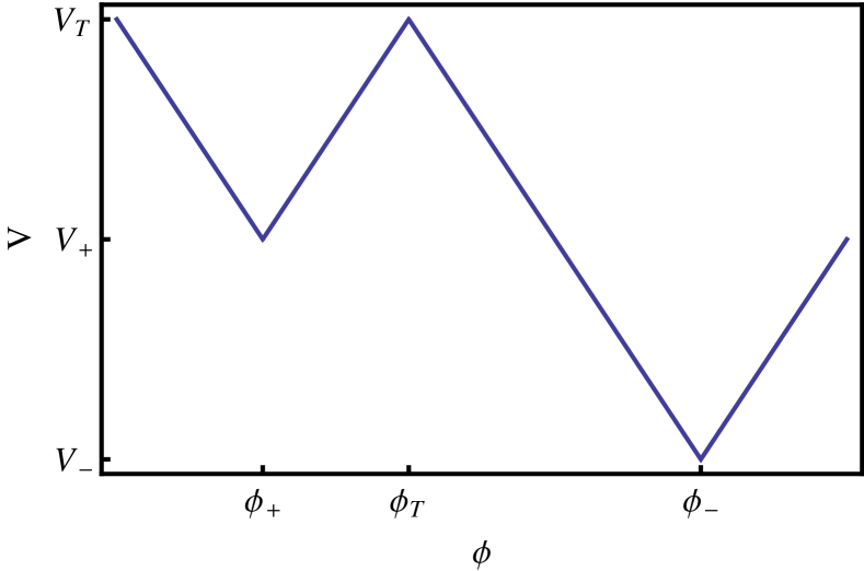
Figure 1: The piecewise linear potential first analyzed by Duncan and Jensen (1992). For $|\phi_{+}-\phi_{T}|>|\phi_{-}-\phi_{T}|$, the bounce solution can only be found after modifying the initial conditions.

II Existence of bounce solutions

In his pioneering paper Coleman (1977), Coleman offered an existence proof for the bounce solution. We briefly sketch this proof before we specialize to piecewise linear potentials in the next Section.

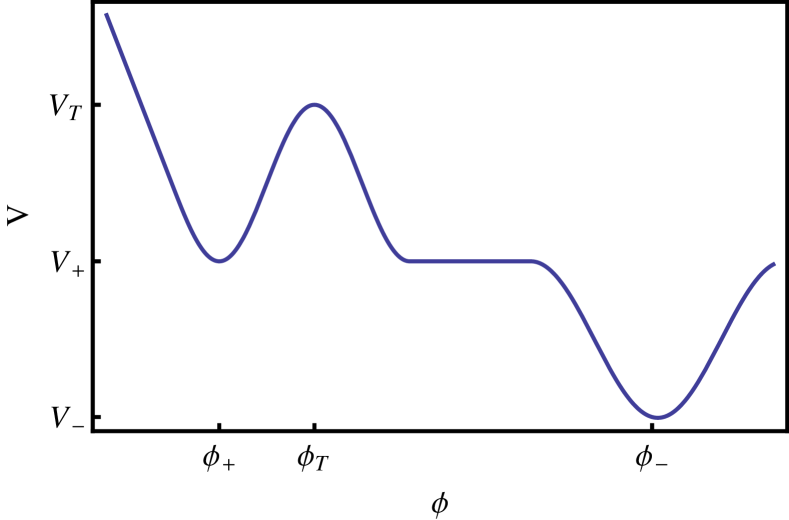
Figure 2: Schematic view of a potential with an existing bounce solution. The crucial part is that the true minimum is a smooth function of $\phi$, i.e. $\partial_{\phi}V$ is continuous.

In the inverted potential (see Figure 2), the bounce solution $\phi_{B}$ is the solution to the equation of motion (in $3+1$ dimensional Euclidean space time)

$$\phi^{\prime\prime}+\frac{3}{r}\phi^{\prime}-\partial_{\phi}V = 0\,,$$ (1)

where $\phi^{\prime}\equiv\partial_{r}\phi$ with the following properties. At the center of the bubble, at $r=0$, the field sits with zero velocity at position $\phi_{0}$ somewhere between $\phi_{T}$, the location of the top of the potential barrier, and $\phi_{-}$, the location of the true vacuum. For $r>0$, the field moves towards the false vacuum $\phi_{+}$, reaching it with zero speed for $r\to\infty$. Owing to the friction term in Eq. (1), it is not immediately clear that the field can ever reach $\phi_{+}$.

Inside of the bubble, starting ever closer to $\phi_{-}$, the field can sit almost fixed at that position for a longer and longer time – until friction dies off. Then, energy conservation makes the field roll past $\phi_{+}$ as long as $\Delta V_{-}\geq\Delta V_{+}$ ($\phi_{\pm}$ being the location of the false and true vacuum respectively, and $\Delta V_{\pm}=V_{T}-V_{\pm}$). To show that overshooting past $\phi_{+}$ occurs for starting values $\phi_{0}$ close enough to $\phi_{-}$, we need to be somewhat quantitative: For analytic potentials it is possible to linearize the equation of motion close to the true vacuum $\phi_{-}$, giving

$$\left(\partial_{r}^{2}+\frac{3}{r}\partial_{r}-\mu^{2}\right)(\phi-\phi_{-}) = 0\,,$$ (2)

with $\mu^{2}=V^{\prime\prime}(\phi_{-})$. It is solved by

$$\phi(r)-\phi_{-} = 2(\phi_{0}-\phi_{-})\frac{I_{1}(\mu r)}{\mu r}\,,$$ (3)

where $I_{1}$ is the Bessel function of the first kind, see Coleman (1977). Hence for $\phi_{0}$ ever closer to $\phi_{-}$, the field can sit near $\phi_{-}$ for larger and larger $r$. Making the initial displacement from $\phi_{-}$ sufficiently small, $r$ becomes large enough such that the friction term effectively disappears. Thus by energy conservation, $\phi$ can rush past $\phi_{+}$.

On the other hand, starting far away from the top of the inverted potential, the field does not have enough energy to climb up to $\phi_{+}$. Thus, by continuity, there must be an initial value $\phi_{0}$ being $\phi_{T}<\phi_{0}<\phi_{-}$ such that the field reaches $\phi_{+}$ with zero velocity.

III Piecewise linear potentials

The existence of the bounce crucially depends on the possibility of the field to spend arbitrarily long times arbitrarily close to the true vacuum. In other words, if the equation of motion (2) takes on a different form, it is not guaranteed that the field can spend enough time near the true minimum for the friction term to die out. In particular, it is intuitively clear that this is the case for piecewise linear potentials, see Figure 1. In the following, we discuss the tunneling solutions in detail for a piecewise linear potential, pointing out several subtleties before we analyze the transition to the smooth and regular potential where the kinks are resolved by caps.

Tunneling in a piecewise linear potential

$$V = \left\{\begin{array}[]{cc}V_{T}+\lambda_{+}(\phi-\phi_{T})\,,&\phi<\phi_{T}\\ V_{T}-\lambda_{-}(\phi-\phi_{T})\,,&\phi\geq\phi_{T}\end{array}\right.\,,$$ (6)

has been analyzed by Duncan and Jensen (1992), see Figure 1. We present their analysis in a slightly different form.

First of all, we set $\phi_{T}=V_{T}=0$ as shifts in the field and in the zero point energy do not change the physics – ignoring the effects of gravity. Solving the equation of motion inside of the bubble

$$\phi_{i}^{\prime\prime}+\frac{3}{r}\phi_{i}^{\prime}+\lambda_{-} = 0\,,$$ (7)

subject to $\phi(0)=\phi_{0}$, $\phi^{\prime}(0)=0$, we find

$$\phi_{i} = \phi_{0}-\frac{\lambda_{-}}{8}r^{2}\,.$$ (8)

Enforcing the matching condition $\phi_{i}(R_{T})=0$ gives

$$R_{T} = 2\sqrt{\frac{2\phi_{0}}{\lambda_{-}}}\,.$$ (9)

Solving the equation of motion on the outside of the bubble

$$\phi_{o}^{\prime\prime}+\frac{3}{r}\phi_{o}^{\prime}-\lambda_{+} = 0\,,$$ (10)

subject to $\phi_{o}(R_{T})=0$, $\phi_{o}^{\prime}(R_{T})=\phi_{i}^{\prime}(R_{T})$, we find

$$\phi_{o} = \frac{(R_{T}^{2}-r^{2})(R_{T}^{2}(\lambda_{-}+\lambda_{+})-r^{2}\lambda_{+})}{8r^{2}}\,.$$ (11)

On the outside, the field settles in the false vacuum at radius $R_{+}>R_{T}$, for which $\phi_{o}^{\prime}(R_{+})=0$

$$R_{+} = \left(1+\frac{\lambda_{-}}{\lambda_{+}}\right)^{1/4}R_{T}\,.$$ (12)

At this position, the field has the value

$$\phi_{o}(R_{+}) \equiv \phi_{+}=-\phi_{0}\frac{\sqrt{1+c}-1}{\sqrt{1+c}+1}\,,$$ (13)

where $c=\lambda_{-}/\lambda_{+}$. As $\phi_{0}<\phi_{-}$, this gives a restriction on the shape of the potential

$$\alpha\equiv\frac{-\phi_{+}}{\phi_{-}}\leq\frac{-\phi_{+}}{\phi_{0}}=\frac{\sqrt{1+c}-1}{\sqrt{1+c}+1}<1\,.$$ (14)

This is equivalent to

$$\frac{\Delta V_{+}}{\Delta V_{-}} \leq \frac{1}{2+c+2\sqrt{1+c}}\leq\frac{1}{4}\,.$$ (15)

In other words, the bounce solutions given by Eq. (8) and Eq. (11) with initial condition $\phi(0)=\phi_{0}$, $\phi^{\prime}(0)=0$ are only valid for the parameter range $\alpha<1$ and $\Delta\equiv\Delta V_{+}/\Delta V_{-}<\frac{1}{4}$.

As was already pointed out by Duncan and Jensen (1992), outside of this parameter range, the initial conditions need to be modified to find a bounce solution. These modifications are explored in more detail below. But before proceeding, let us take a look at the physical meaning of these conditions. It corresponds to a potential profile where the energy difference between the false and the true vacuum is large (i.e.  not thin-wall) and $|\phi_{+}|<|\phi_{-}|$. In this case, it is always possible to find a field position $\phi_{0}<\phi_{-}$ with zero initial velocity such that the field can roll up the hill to $\phi_{+}$.

On the other hand, if either $\Delta>1/4$ for any value of $\alpha$, or $\Delta<1/4$ and $\alpha>1$, it is not immediately clear that a bounce solution exists for $\phi_{0}\leq\phi_{-}$. The physical picture is as follows:

For $\Delta>1/4$ (and any value of $\alpha$), there is a smaller energy difference between the true and the false minimum – in the extreme case, making the energy difference infinitesimally small for $\Delta\to 1$, the thin-wall limit. For almost degenerate minima, the field would need to wait near the true minimum for the friction term to fall off. But the linear potential makes it impossible for the field to stay longer at that initial position. Therefore, with a small energy difference between the true and the false vacuum, the field can not roll up the hill due to friction, and no solution exists that reaches $\phi_{+}$.

For $\Delta<1/4$ and $\alpha>1$, although the field has a large potential energy to start with, the non-vanishing friction term still prevents it from climbing up the long shallow part to reach $\phi_{+}$.

Another example in which a large difference in potential energy does not guarantee a bounce solution are scalar potentials with local $\phi^{4}$ (or higher power) behavior

$$V = -\frac{c_{4}}{4}(\phi-\phi_{*})^{4}+\text{higher order}\,,\quad c_{4}>0\,.$$ (16)

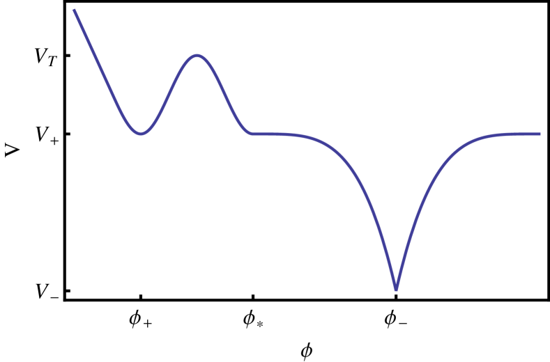
Figure 3: Shape of a true minimum for which no bounce exists. If the wings of the trough at $\phi_{-}$ are polynomials of at least order $4$, the bounce solution in the inverted potential cannot roll past the point $\phi_{*}$ on the left.

For solutions to the equation of motion

$$\phi^{\prime\prime}+\frac{3}{r}\phi^{\prime}+c_{4}(\phi-\phi_{*})^{3} = 0\,,$$ (17)

with initial conditions $\phi(0)=\phi_{0}$ and $\phi^{\prime}(0)=0$, the field reaches $\phi=\phi_{*}$ with zero speed Dutta et al. (2011) independent from the release point $\phi_{0}$. If the $\phi^{4}$ behavior ends with a kink (as depicted in Figure 3) no bounce solution exists.

It is important to note that the arguments illustrated in Section II do not immediately hold here: there is no quadratic approximation of the potential around the true minimum to get Eq. (2). In a linear potential, putting the initial position ever closer to the true minimum $\phi_{-}$ does not force the field to spend an ever longer time there.

As Duncan and Jensen (1992) pointed out, one thus needs to modify the initial conditions. Inside the bubble, the field should be artificially fixed at the true minimum $\phi_{-}$ until radius $R_{0}$. This should be understood as an approximation. In particular, this can be interpreted as mimicking the effect of removing the kink and replacing it with a smooth cap. In this suitably capped potential, the field can sit arbitrarily close to the true minimum and spend ever longer time there. It is clear that the original argument of the existence of bounce solution as outlined in Section II immediately holds.

This waiting period can be realized by a change in the boundary conditions as first done by Duncan and Jensen (1992) for a piecewise linear potential. The modified initial conditions become $\phi_{i}(r)=\phi_{-}$, $\phi_{i}^{\prime}(r)=0$ for $0\leq r\leq R_{0}$, giving

$$\phi_{i}(r) = \phi_{-}-\frac{(r^{2}-R_{0}^{2})^{2}}{8r^{2}}\lambda_{-}\,$$ (18)

for $R_{0}\leq r<R_{T}$. Outside of the bubble at $R_{+}>R_{T}$, the field comes to rest in the false vacuum $\phi_{o}^{\prime}(R_{+})=0$, $\phi_{o}^{\prime}(R_{+})=0$, giving

$$\phi_{o}(r) = \phi_{+}+\frac{(r^{2}-R_{+}^{2})^{2}}{8r^{2}}\lambda_{+}\,.$$ (19)

Now matching the two solutions $\phi_{i}(R_{T})=0=\phi_{o}(R_{T})$, $\phi_{i}^{\prime}(R_{T})=\phi_{o}^{\prime}(R_{T})$ gives

$$R_{0} = \frac{\phi_{-}}{1-\sqrt{\Delta}}\sqrt{\frac{2}{V_{-}}}\sqrt{(1+\alpha)\left[\alpha-1+2\sqrt{\Delta}\right]}\,,$$

$$R_{T} = \frac{\phi_{-}}{1-\sqrt{\Delta}}\sqrt{\frac{2}{V_{-}}}(1+\alpha)\,,$$ (20)

$$R_{+} = \frac{\phi_{-}}{1-\sqrt{\Delta}}\sqrt{\frac{2}{V_{-}}}\sqrt{(1+\alpha)\left[1+\alpha\left(\frac{2}{\sqrt{\Delta}}-1\right)\right]}\,,$$

with $R_{0}<R_{T}<R_{+}$, $\alpha=-\frac{\phi_{+}}{\phi_{-}}$, $\Delta V_{\pm}=V_{T}-V_{\pm}$ and $\Delta=\frac{\Delta V_{+}}{\Delta V_{-}}$. Note that the condition that $R_{0}$ is real implies that $\alpha>1-2\sqrt{\Delta}$.

The tunneling amplitude can then be computed as

$$B = B_{a}+B_{b}+B_{c}\,,$$ (21)

with

$$B_{a} = 2\pi^{2}\int_{0}^{R_{0}}\!dr\,r^{3}\left(-\lambda_{-}\phi_{-}-\lambda_{+}\phi_{+}\right)\,,$$ (22)

$$B_{b} = 2\pi^{2}\int_{R_{0}}^{R_{T}}\!dr\,r^{3}\left(\frac{1}{2}\phi_{L}^{\prime 2}-\lambda_{-}\phi_{L}-\lambda_{+}\phi_{+}\right)\,,$$ (23)

$$B_{c} = 2\pi^{2}\int_{R_{T}}^{R_{+}}\!dr\,r^{3}\left(\frac{1}{2}\phi_{R}^{\prime 2}+\lambda_{+}\phi_{R}-\lambda_{+}\phi_{+}\right)\,,$$ (24)

giving

$$B = \frac{2\pi^{2}}{3}\frac{\phi_{-}^{4}}{\Delta V_{-}}\frac{(1+\alpha)^{3}\left((\alpha-3)\sqrt{\Delta}+1-3\alpha\right)}{(\sqrt{\Delta}-1)^{3}}\,.$$ (25)

For certain choices of parameters of a piecewise linear potential, we just saw that the bounce solutions exist only when we keep the field artificially fixed at the true minimum. Holding it there for a sufficiently long time, the damping term becomes small enough such that the field can reach the false vacuum with zero velocity. This should be thought of as an approximation to the physical situation of smoothing the tip with a cap.

IV Caps versus kinks

In this Section, we discuss in which cases replacing the tip of a piecewise linear potential with a smooth cap can be well approximated by keeping the field artificially fixed at the minimum as outlined in the previous Section. This means that the original argument by Coleman guarantees the existence of a bounce. Here we focus on the error in the tunneling action which is introduced by the kink approximation.

Suppose that a piecewise linear potential is obtained as the limit of a regular smooth potential. The scale $\delta\phi$ on which the kink is resolved in the regular potential serves as expansion parameter $\delta\phi\ll|\phi_{T}-\phi_{-}|$. Apparently, the bounce actions can be very different, if the smooth potential varies strongly in the cap region. For example, if the potential has a large positive spike, the bounce solution can leave the cap region with a sizable velocity that can alter the bounce action significantly. Hence we demand that the potential in the cap does not differ too much from the corresponding value $V_{-}$ in the kink potential at least up to the first local minimum in the regularized potential

$$|V_{-}^{\rm{cap}}-V^{\rm{kink}}_{-}|\lesssim\lambda_{-}\delta\phi.$$ (26)

Still, the potential can vary strongly in the cap region in the sense that its derivative does not need to be small. Some examples are given in Figure 4.

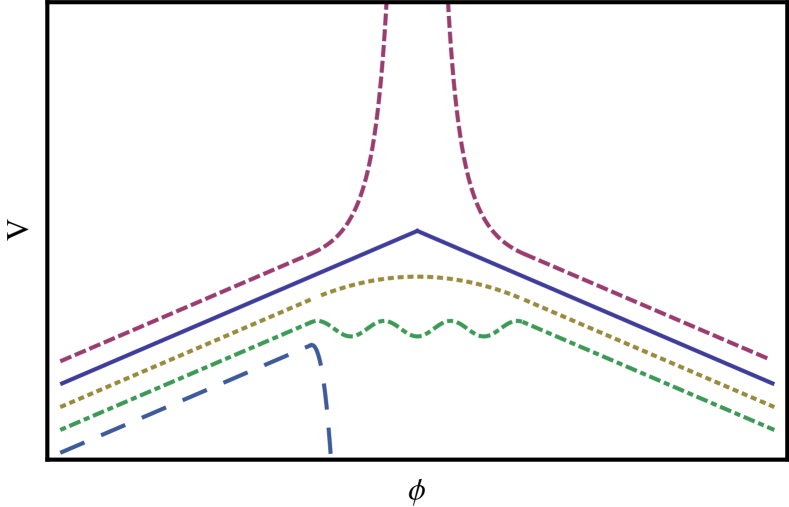
Figure 4: The piecewise linear potential and different regular potentials in the cap region. The three potentials on the bottom pass the criterion (26) while the potential on top can lead to large deviations in the bounce action.

Now, consider the bounce solutions for the kink potential and the cap potential outside the cap region. Even for large $r$ these two solutions only coincide approximately. It might well be that one of the two solutions passes a given point in the potential a little bit later but compensates by a slightly smaller velocity. The former effect leads to a reduced friction that is compensated by the latter effect.

Even a small difference between the two bounces can have a large effect on the action. To see this, consider a piecewise linear potential with two slightly different kink positions $\phi_{-}$ but same slope $\lambda_{-}$. Suppose that we would arrange this shift in $\phi_{-}$ such that the bounce solution of this modified kink potential and the bounce of the regular potential coincide. The potential with the more remote kink position $\phi_{-}$ has a smaller $R_{0}$. According to (25), a shift $\Delta\phi_{-}$ leads generically to a change in the bounce action of order $\delta B/B\sim\Delta\phi_{-}/\phi_{-}$ and hence be small. Only in the thin wall regime where $\Delta\simeq 1$ this change can be large and of order

$$\frac{\delta B}{B}\simeq\frac{3}{2}\frac{1}{\sqrt{\Delta}-1}\frac{\Delta\phi_{-}}{\phi_{-}}.$$ (27)

Fortunately, $\Delta\phi_{-}$ cannot be larger than $\delta\phi$. We prove this by contradiction. The solution to the field equations of motion are (see Eq. (18))

$$\phi_{i}(r) = \phi_{-}+\Delta\phi_{-}-\frac{(r^{2}-(R_{0}+\delta R_{0})^{2})^{2}}{8r^{2}}\lambda_{-}\ .$$ (28)

Now assume $\delta\phi\ll\Delta\phi_{-}\ll\phi_{-}$: the field leaves the cap at

$$r^{2}-(R_{0}+\delta R_{0})^{2}\simeq\sqrt{8\Delta\phi_{-}(R_{0}+\delta R_{0})^{2}/\lambda_{-}}$$ (29)

with velocity

$$\phi_{i}^{\prime}\simeq\sqrt{2\Delta\phi_{-}\lambda_{-}}.$$ (30)

However, due to energy conservation and the condition (26), the energy at the border of the cap cannot exceed the potential energy. This implies

$$\phi_{i}^{\prime}\lesssim\sqrt{2\lambda_{-}\delta\phi},$$ (31)

and hence $\Delta\phi_{-}\lesssim\delta\phi$ such that

$$\frac{\delta B}{B}\lesssim\frac{3}{2}\frac{1}{\sqrt{\Delta}-1}\frac{\delta\phi}{\phi_{-}}\,.$$ (32)

Thus we demand

$$\sqrt{\Delta}-1\gg\frac{\delta\phi}{\phi_{-}},$$ (33)

in order to obtain accurate results for the bounce action in the kink approximation.

Even though our reasoning above seems very conservative, no better upper bound on the variation of the action exists in the thin-wall regime. The boundary of the relation (33) is equivalent to

$$|V_{+}-V_{-}|\simeq\lambda_{-}\delta\phi\,,$$ (34)

but in this case the potential difference between the true and false vacua in the regular capped potential can be very different from that in the kink potential. This can lead to grossly different bounce actions. For this special situation, the constraint in (32) is saturated.

Combining the criteria (26) and (33), our two conditions on the kink approximation read

$$|V_{-}^{\rm cap}-V^{\rm kink}_{-}|\lesssim\lambda_{-}\delta\phi\ll|V^{\rm kink}_{+}-V^{\rm kink}_{-}|\,.$$ (35)

In general, the kink approximation turns out to be very robust, as eq. (35) only limits strong variations of the scalar potential within the smooth ’ cap’ region. The exception to the general case is given by the thin-wall limit. There, the tunneling action depends sensitively on the bubble wall tension and the vacuum energy difference. Hence, in this regime the thin-wall approximation is more appropriate. The kink approximation agrees with the thin-wall limit if it keeps constant the bubble wall tension and the vacuum energy difference.

V Exotic caps

In the preceding Sections, we demonstrated that under most circumstances, smoothing the kink in a piecewise linear potential is equivalent to holding the field fixed at some radius $R_{0}$. This statement depends crucially on the choice of cap that replaces the kink. The shape of the cap must be such that the field can spend an arbitrarily long time $R$ close to the true vacuum to allow the friction term to get sufficiently small. This time $R$ is approximately (assuming that friction dominates over acceleration in the equation of motion)

$$\frac{3}{r}\frac{d\phi}{dr}\approx V^{\prime}(\phi) \Rightarrow \int_{\phi_{0}}^{\phi(R)}\!\!\frac{d\phi}{V^{\prime}(\phi)}=\frac{1}{6}R^{2}\,.$$ (36)

To spend an arbitrary and potentially infinite amount of time near the cap, the integral must diverge in the limit $\phi_{0}\to\phi_{-}$. Certainly this is true for analytic potentials with a finite mass $|V^{\prime\prime}(\phi_{-})|<\infty$. For example, taking $V(\phi)=\frac{1}{2}m^{2}\phi^{2}$, it is clear that the integrand becomes $1/V^{\prime}(\phi)=1/m^{2}\phi$ which is logarithmically divergent.

However, potentials such that the integral is finite in the limit $\phi_{0}\to\phi_{-}$ do also exist. One class of examples are potentials of the form $V\propto|\phi-\phi_{-}|^{\alpha}$, with $1<\alpha<2$, which we shall now analyze in more detail. The derivative of the potential at the minimum is $V^{\prime}(\phi_{*})=0$ in the limit $\phi_{*}\to\phi_{-}$ both from the left and from the right.

To set up the full picture, let us assume a piecewise potential, where we examine the area around the cap. We assume that the other piecewise parts of the potential contain at least one other local minimum. The complete bounce is given by matching the solutions in each part of the potential. We solve the equations of motion for the bounce in the part of the potential describing the cap where $V(\phi)=\lambda|\phi-\phi_{-}|^{\alpha}$, $1<\alpha<2$. The equation of motion reads

$$\phi^{\prime\prime}+\frac{3}{r}\phi^{\prime}-\lambda\alpha\mathop{\mathrm{sgn}}(\phi-\phi_{-})|\phi-\phi_{-}|^{\alpha-1} = 0\,,$$ (37)

subject to the boundary conditions $\phi(0)=\phi_{0},\,\phi^{\prime}(0)=0$. Even in the limit $\phi_{0}\to\phi_{-}$, the solution spends only a finite amount of time in the cap region and is given by

$$\phi(r) = \phi_{-}+\left(\frac{4\alpha\lambda(\alpha-2)^{2}}{3-\alpha}\right)^{\frac{1}{2-\alpha}}r^{\frac{2}{2-\alpha}}\,.$$ (38)

Hence, even though the field starts off from the extremum where there is no force ($V^{\prime}(\phi_{-})=0$), it begins rolling away in finite time. However, this does not imply that there is no bounce. The field can wait for some time at $\phi_{-}$ and then still leave the cap in finite time (friction is even less important than in the previous case). This solution can be obtained by using the boundary conditions $\phi(R_{0})=\phi_{0}$ and $\phi^{\prime}(R_{0})=0$, and sending the release point subsequently to $\phi_{-}$. If the waiting period $R_{0}$ is chosen appropriately, the field reaches the false vacuum, thus constituting a bounce solution.

Numerically, the bounce solution is often determined using the shooting algorithm Coleman (1977). In this case, a release position for the field is chosen and the corresponding initial value problem using the equation of motion is solved. The release point is then varied until the correct boundary conditions of the bounce solution in the false vacuum are fulfilled. Obviously, a bounce of the kind described above cannot be found with the conventional shooting algorithm.

This situation might be rather surprising, since the potential is smooth and even differentiable everywhere. This special situation arises because the equation of motion for the bounce in the potential (37) with $\alpha<2$ does not fulfill the Lipschitz condition. Hence the Picard-Lindelöf theorem does not hold and a solution to the initial value problem is not necessarily unique. This kind of situation is well known in the philosophy of science community Norton (2008) in the context of classical mechanics. Fortunately, here we need not concern ourselves with the initial value problem. We are interested in computing the tunneling amplitude, and the bounce solution with the usual boundary conditions is indeed unique. So for this kind of smooth and regular potential, one can be in the situation that the kink approximation describes the tunneling process quite well, while the common shooting algorithm fails.

VI Conclusions

We have addressed the range of validity the kink approximation to Coleman tunneling in a smooth potential. Tunneling in a piecewise linear potential with kings was first discussed analytically in Duncan and Jensen (1992). For certain ranges of parameters, a consistent bounce solution exists only if the field can rest for some amount of Euclidean time at the true vacuum. With this field profile, it is possible for the relevant friction term to die off sufficiently so that the field can roll back up to the false vacuum. Having the field ’wait’ in such a manner is only an approximation to the full bounce solution where the tip represents a smooth cap of a regular potential.

We found that replacing a regular smooth potential by its piecewise linear approximation is a very robust procedure. A sufficient criterion for the bounce action of the kink potential to yield accurate results is given by

$$|V_{-}^{\rm{cap}}-V^{\rm{kink}}_{-}|\lesssim\lambda_{-}\delta\phi\ll|V^{\rm kink}_{+}-V^{\rm kink}_{-}|\,.$$ (39)

Here, $\delta\phi$ is the scale on which the kink is resolved in the smooth and regular potential, $\lambda_{-}$ denotes the slope in the kink potential close to the true minimum and $V_{\mp}$ denote values of the potential in the true (false) vacuum, respectively.

The first inequality reflects the fact that the bounce action varies strongly if the field can accumulate a sizable kinetic energy in the cap; the second inequality results from the fact that the bounce action is very sensitive to the potential difference between the true and the false vacuum in the thin-wall regime.

For example, this includes potentials that fluctuate strongly or that do not have a finite second derivative in the true vacuum, as for potentials that behave close to the true vacuum as $V\simeq(\phi-\phi_{-})^{\alpha}$ with $1<\alpha<2$. In particular, for the latter class of potentials, the kink approximation yields accurate results even though the bounce solutions cannot be obtained from the regular potential using the conventional shooting algorithm.

Violations of the condition Eq. (39) can appear for instance within the context of the 4D effective field theory approximation to a theory of quantum gravity such as string theory. It is not clear how to self-consistently describe caps with curvature larger than $M_{p}^{2}$ within this framework. In particular, in such a high curvature cap, steep local maxima acting as large positive spikes as discussed before cannot be excluded. In a situation where the cap is confined to such a region of strong quantum gravity effects, we can no longer guarantee that condition (39) is satisfied from a calculation of the cap from effective field theory. Thus, a description of the tunneling using the description of Coleman (1977) and Coleman and De Luccia (1980) entirely within the realm of effective field theory is not possible for a high curvature cap. In this case, full quantum gravity effects must be incorporated to calculate the tunneling amplitude.

The kink approximation in terms of piecewise linear potentials Duncan and Jensen (1992) was used to estimate the tunneling rate in highly asymmetrical potentials far away from the thin-wall limit. Examples arise in theories of meta-stable dynamical supersymmetry breaking in ${\cal N}=1$ gauge theories Intriligator et al. (2006), or their embedding into heterotic string theory Serone and Westphal (2007). The kink approximation was used there without any prior justification of its validity, and might have led to qualitatively different life times, which motivated our work.

Beyond field theory, possible examples in string theory are e.g. warped compactifications with D3-branes. In such compactifications, the warp factor contributes to the 4D effective scalar potential. To leading order, the warp factor, and in turn its contribution to the 4D scalar potential, may develop ’kinks’ at the position of a D3-brane, similar to the case of 5D warped Randall-Sundrum compactifications Randall and Sundrum (1999). String theory effects can smooth such ’kinks’, but the curvature of the smoothing cap may then be too large, as mentioned above, for a treatment within effective field theory alone.

References

- Coleman (1977) S. R. Coleman, “The Fate of the False Vacuum. 1. Semiclassical Theory”, Phys. Rev. D15 (1977) 2929–2936.
- Callan and Coleman (1977) J. Callan, Curtis G. and S. R. Coleman, “The Fate of the False Vacuum. 2. First Quantum Corrections”, Phys.Rev. D16 (1977) 1762–1768.
- Coleman and De Luccia (1980) S. R. Coleman and F. De Luccia, “Gravitational Effects on and of Vacuum Decay”, Phys.Rev. D21 (1980) 3305.
- Coleman (1988) S. R. Coleman, “QUANTUM TUNNELING AND NEGATIVE EIGENVALUES”, Nucl.Phys. B298 (1988) 178.
- Cvetic and Soleng (1995) M. Cvetic and H. H. Soleng, “Naked singularities in dilatonic domain wall space times”, Phys.Rev. D51 (1995) 5768–5784, arXiv:hep-th/9411170.
- Johnson and Larfors (2008) M. C. Johnson and M. Larfors, “An Obstacle to populating the string theory landscape”, Phys.Rev. D78 (2008) 123513, arXiv:0809.2604.
- Yang (2010) I.-S. Yang, “Stretched extra dimensions and bubbles of nothing in a toy model landscape”, Phys.Rev. D81 (2010) 125020, arXiv:0910.1397.
- Aguirre et al. (2010) A. Aguirre, M. C. Johnson, and M. Larfors, “Runaway dilatonic domain walls”, Phys.Rev. D81 (2010) 043527, arXiv:0911.4342.
- Brown and Dahlen (2010) A. R. Brown and A. Dahlen, “Small Steps and Giant Leaps in the Landscape”, Phys.Rev. D82 (2010) 083519, arXiv:1004.3994.
- Brown and Dahlen (2011) A. R. Brown and A. Dahlen, “The Case of the Disappearing Instanton”, arXiv:1106.0527, * Temporary entry *.
- Randall and Sundrum (1999) L. Randall and R. Sundrum, “A Large mass hierarchy from a small extra dimension”, Phys.Rev.Lett. 83 (1999) 3370–3373, arXiv:hep-ph/9905221, 9 pages, LaTex Report-no: MIT-CTP-2860, PUPT-1860, BUHEP-99-9.
- Kaloper (1999) N. Kaloper, “Bent domain walls as brane worlds”, Phys.Rev. D60 (1999) 123506, arXiv:hep-th/9905210.
- Brummer et al. (2006) F. Brummer, A. Hebecker, and E. Trincherini, “The Throat as a Randall-Sundrum model with Goldberger-Wise stabilization”, Nucl.Phys. B738 (2006) 283–305, arXiv:hep-th/0510113.
- Duncan and Jensen (1992) M. J. Duncan and L. G. Jensen, “Exact tunneling solutions in scalar field theory”, Phys.Lett. B291 (1992) 109–114.
- Dutta et al. (2011) K. Dutta, P. M. Vaudrevange, and A. Westphal, “The Overshoot Problem in Inflation after Tunneling”, arXiv:1109.5182, * Temporary entry *.
- Norton (2008) J. D. Norton, “The dome: An unexpectedly simple failure of determinism”, Philosophy of Science Vol. 75, No. 5 December (2008) 786–798.
- Intriligator et al. (2006) K. A. Intriligator, N. Seiberg, and D. Shih, “Dynamical SUSY breaking in meta-stable vacua”, JHEP 0604 (2006) 021, arXiv:hep-th/0602239.
- Serone and Westphal (2007) M. Serone and A. Westphal, “Moduli Stabilization in Meta-Stable Heterotic Supergravity Vacua”, JHEP 0708 (2007) 080, arXiv:0707.0497.