The frustrated Heisenberg antiferromagnet on the checkerboard lattice:
the $J_{1}$–$J_{2}$ model

Abstract

We study the zero-temperature ground-state (gs) phase diagram of the spin-$\frac{1}{2}$ anisotropic planar pyrochlore (or crossed chain) model using the coupled cluster method (CCM). The model is equivalently described as a frustrated $J_{1}$–$J_{2}$ antiferromagnet on the two-dimensional checkerboard lattice, with nearest-neighbor exchange bonds of strength $J_{1}>0$ and next-nearest-neighbor bonds of strength $J_{2}\equiv\kappa J_{1}>0$. Using various antiferromagnetic (AFM) classical ground states as CCM model or reference states we present results for the gs energy, average on-site magnetization, and the susceptibilities of these states against the formation of plaquette valence-bond crystal (PVBC) and crossed-dimer valence-bond crystal (CDVBC) ordering. Our calculations show that the AFM quasiclassical state with Néel ordering is the gs phase for $\kappa<\kappa_{c_{1}}\approx 0.80\pm 0.01$, but that none of the fourfold set of AFM states that are selected by quantum fluctuations at $O(1/s)$ in a large-$s$ analysis (where $s$ is the spin quantum number) from the infinitely degenerate set of AFM states that form the gs phase for the classical version ($s\to\infty$) of the model (for $\kappa>1$) survives the quantum fluctuations to form a stable magnetically-ordered gs phase for the $s=\frac{1}{2}$ case. We show that the quasiclassical Néel state becomes infinitely susceptible to PVBC ordering at or very near to $\kappa=\kappa_{c_{1}}$, and that the quasiclassical fourfold AFM states become infinitely susceptible to PVBC ordering at $\kappa=\kappa_{c_{2}}\approx 1.22\pm 0.02$. In turn, we find that these states become infinitely susceptible to CDVBC ordering for all values of $\kappa$ above a certain critical value at or very near to $\kappa=\kappa_{c_{2}}$. Our calculations thus indicate a Néel-ordered gs phase for $\kappa<\kappa_{c_{1}}$, a PVBC-ordered phase for $\kappa_{c_{1}}<\kappa<\kappa_{c_{2}}$, and a CDVBC-ordered phase for $\kappa>\kappa_{c_{2}}$. Both transitions are likely to be direct ones, although we cannot exclude very narrow coexistence regions confined to $0.79\lesssim\kappa\lesssim 0.81$ and $1.20\lesssim\kappa\lesssim 1.22$ respectively.

I INTRODUCTION

The theoretical study of two-dimensional (2D) frustrated quantum antiferromagnets has been strongly motivated by the fact that such quantum spin models often describe well the properties of real magnetic materials of great experimental interest. These models have also become of huge current interest because the interplay between frustration and quantum fluctuations seen in them can produce, even at zero temperature ($T=0$), a wide variety of fascinating quantum phases ranging from those with quasiclassical ordering to valence-bond solids and spin liquids.Sachdev:1995 ; 2D_magnetism_1 ; 2D_magnetism_2 They have thus become paradigms of systems that may be used to study quantum phase transitions between quasiclassical phases showing magnetic order and magnetically disordered quantum phases.

Some of the parameters that determine which type of ordering occurs include the lattice geometry, the dimensionality $D$ of the system, the spin quantum number $s$ of the atoms situated on the lattice sites, the number and range of the magnetic bonds, and the degree to which bond frustration of either the geometric or dynamical kind is present. New impetus for the study of 2D quantum spin-lattice models comes from recent proposals to realize them experimentally with ultracold atoms trapped in an optical lattice.Struck:2011 The particularly exciting scenario thus opens of being able to tune the competing bond strengths and thus to investigate experimentally the ensuing quantum phase transitions and their dynamics.

One of the prime theoretical interests in frustrated quantum magnets lies in the possibility that they might exhibit quantum disordered states and/or spin-liquid behavior. Among the most highly frustrated, and hence most promising, candidate systems in this regard are those that are composed of tetrahedra coupled into two-dimensional (2D) or three-dimensional (3D) lattice networks. Prominent among the latter are the pyrochlores, whose basic structure is one of vertex-sharing tetrahedra. Indeed, experiments on such $s=\frac{1}{2}$ pyrochlores as Y₂Ir₂O₇ do seem to show evidence for a quantum spin-liquid state.Fukuzawa:2003

In order to reduce the complexity of the 3D pyrochlore lattice, but without diminishing the magnetic frustration, one may project the 3D vertex-sharing lattice of tetrahedra onto a 2D plane. Each tetrahedron comprises four spins at its vertices, with each of its six edges or links representing an interaction of the Heisenberg antiferromagnet (HAFM) form. Each such tetrahedron is thus mapped to a square with spins at its vertices and with sides representing antiferromagnetic (AFM) bonds, but now with additional AFM links across its diagonals. Such a pattern is repeated in the vertex-sharing arrangement shown in the checkerboard pattern of Fig. 1.

     

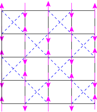
(a) Néel

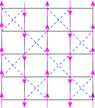
(b) striped

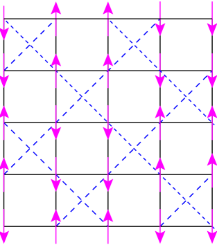
(c) Néel^∗

Figure 1: (Color online) The $J_{1}$–$J_{2}$ checkerboard model (with $J_{1}=1$), showing (a) the Néel state, (b) the (columnar) striped state and (c) one of the two Néel^∗ states. The NN $J_{1}$ bonds are shown as solid (black) lines and the NNN $J_{2}$ bonds are shown as dashed (blue) lines. The arrows represent the orientations of the spins on each lattice site for each of the three states shown.

Although this 2D projection of the 3D pyrochlore structure preserves its vertex-sharing structure, the symmetry in the 3D structure between the six bonds on each tetrahedron is lost in the 2D projection since the two diagonal bonds of each crossed square are now inequivalent to the four bonds on the sides of the square. This subsequent reduction in the symmetry is thus consistent with considering an anisotropic Heisenberg model on the 2D checkerboard lattice in which the AFM exchange interactions along the sides of the squares (with strength $J_{1}>0$) are generally different in strength from those along the diagonals of the crossed squares (which have a strength $J_{2}>0$), as shown in Fig. 1. The resulting frustrated model is thus called the anisotropic planar pyrochlore. Alternative names are the anisotropic checkerboard HAFM, the $J_{1}$–$J_{2}$ checkerboard model, and the crossed chain model.

Although, the spin-$\frac{1}{2}$ anisotropic planar pyrochlore has been studied by a large number of authorsSingh:1998 ; Palmer:2001 ; Chung:2001 ; Brenig:2002 ; Canals:2002 ; Starykh:2002 ; Sindzingre:2002 ; Fouet:2003 ; Berg:2003 ; Tchernyshyov:2003 ; Moessner:2004 ; Hermele:2004 ; Brenig:2004 ; Bernier:2004 ; Starykh:2005 ; Schmidt:2006 ; Arlego:2007 ; Moukouri:2008 ; Chan:2011 the structure of its full phase diagram still remains unsettled and contentious, especially for larger values of the frustration parameter, $\kappa\equiv J_{2}/J_{1}\gtrsim 1$, as we discuss more fully below in Sec. II. Various methods have been applied to the model for different regions of the parameter space for the variable $\kappa$. These include semiclassical ($s\gg 1$) analyses,Singh:1998 ; Canals:2002 ; Tchernyshyov:2003 large-$N$ expansions of the Sp($N$) model,Chung:2001 ; Moessner:2004 ; Bernier:2004 high-order cluster-based strong-coupling series expansion (SE) techniquesBrenig:2002 ; Brenig:2004 ; Arlego:2007 using a continuous unitary transformation generated by the flow equation method of Wegner,Wegner:1994 a real-space renormalization techniqueBerg:2003 using the contractor renormalization method of Morningstar and Weinstein,Morningstar:1996 an easy-axis generalization of the 3D model,Hermele:2004 a quasi-one-dimensional approach (valid in the $\kappa\gg 1$ limit) based on the random phase approximation backed up by a bosonization study,Starykh:2002 techniques that combine renormalization group ideas with one-dimensional bosonization and current algebra methods,Starykh:2005 exact diagonalization (ED) of small finite-lattice clusters,Palmer:2001 ; Sindzingre:2002 ; Fouet:2003 ; Schmidt:2006 a two-step density-matrix renormalization group method,Moukouri:2008 and, very recently, a tensor network simulationChan:2011 based on infinite projected entangled pair states.Jordan:2008

In this paper we use the coupled cluster method (CCM) of quantum many-body theory (see, e.g., Refs. [Bi:1991, ; Bi:1998, ; Fa:2004, ] and references cited therein) to study the spin-$\frac{1}{2}$ $J_{1}$–$J_{2}$ Heisenberg model on the checkerboard lattice, in order to attempt to shed more light on it. The CCM has proven itself in many applications to frustrated magnetic systems to be capable of providing accurate estimates of the quantum critical points marking the phase transitions between states of widely differing order (see e.g., Refs. [Ze:1998, ; Kr:2000, ; ccm3, ; Fa:2001, ; schmalfuss, ; Fa:2004, ; rachid05, ; darradi08, ; Bi:2008_JPCM, ; Bi:2008_PRB, ; richter10, ; UJack_ccm, ; Reuther:2011_J1J2J3mod, ; Farnell:2011, ; Gotze:2011, ]). In view of the continuing interest in the model and the controversy over its $T=0$ phase structure, especially at large frustration ($\kappa\gtrsim 1$), it seems appropriate and timely to bring to bear on the problem the proven power of the CCM. Since, as we shall see, we are able to calculate to high orders in the relevant CCM approximation scheme, as discussed below in Sec. III, we are able to present accurate results from a method of well-proven ability to deal with such strongly correlated and highly frustrated systems.

We now briefly outline the structure of the remainder of the paper. In Sec. II the model itself is first described and discussed. The CCM formalism is then briefly outlined in Sec. III before we present and discuss our CCM results in Sec. IV. Finally, we conclude in Sec. V with a summary of our findings and a comparison of our results for the model with those from other methods.

II THE MODEL

The Hamiltonian for the anisotropic checkerboard-lattice model considered here is given by

$$H=J_{1}\sum_{\langle i,j\rangle}\mathbf{s}_{i}\cdot\mathbf{s}_{j}+J_{2}\sum_{\langle\langle i,k\rangle\rangle}\mathbf{s}_{i}\cdot\mathbf{s}_{k}\,.$$ (1)

where the index $i$ runs over all sites of a square lattice, index $j$ runs over all nearest-neighbor (NN) sites to site $i$, and index $k$ runs over all next-nearest-neighbor (NNN) sites to site $i$ on a checkerboard pattern such that alternate square plaquettes have either two NNN (diagonal) bonds or none, as shown in Fig. 1. The sums over $\langle i,j\rangle$ and $\langle\langle i,k\rangle\rangle$ count each pairwise bond once and once only. Each site $i$ of the lattice carries a particle with spin $s=\frac{1}{2}$ and a spin operator ${\bf s}_{i}=(s_{i}^{x},s_{i}^{y},s_{i}^{z})$.

The lattice and exchange bonds of the anisotropic checkerboard-lattice model are shown in Fig. 1. We may alternatively view the model as comprising crossed (diagonal) sets of chains on which the intrachain exchange coupling constant is $J_{2}$, coupled by (vertical and horizontal) interchain exchange bonds of strength $J_{1}$. We assume here that both bonds are antiferromagnetic (AFM) in nature (i.e., have positive exchange coupling constants) and hence frustrate one another. The model thus interpolates continuously between the isotropic HAFM on the square lattice (when $\kappa\equiv J_{2}/J_{1}=0$) and decoupled one-dimensional (1D) isotropic HAFM chains (when $\kappa\to\infty$). In between, at $\kappa=1$, we have the isotropic HAFM on the checkerboard lattice that is a 2D analog of the 3D isotropic pyrochlore HAFM. Henceforth, without loss of generality, we set $J_{1}\equiv 1$ in order to set the energy scale.

The classical ground-state (gs) phase for this model for $\kappa<1$ is the Néel state shown in Fig. 1(a), in which every column and row exhibits Néel AFM ordering, $\cdots\uparrow\downarrow\uparrow\downarrow\cdots$, and consequently the ordering along each diagonal is ferromagnetic (FM), i.e., where all the spins are aligned parallel to one another. The Néel state has an energy per spin given by $E^{\rm cl}/N=s^{2}(-2J_{1}+J_{2})$. For $\kappa>1$ there is an infinitely degenerate family of collinear gs phases in which every diagonal exhibits Néel AFM ordering, but where every diagonal, each of which is connected by $J_{1}$ bonds to two other crossed diagonals, can be arbitrarily moved along its own direction. These states all have the same energy per spin of $E^{\rm cl}/N=-s^{2}J_{2}$, independent of the exchange coupling $J_{1}$. The classical phase transition is clearly at $\kappa_{{\rm cl}}=1$ ($J_{1}>0$).

Among this infinitely degenerate family of classical states for $\kappa>1$ are the so-called (columnar) striped state shown in Fig. 1(b) and the Néel^∗ state shown in Fig. 1(c). The columnar (row) striped states have FM ordering along columns (rows) but AFM Néel ordering along rows (columns). The Néel^∗ state has doubled AFM ordering, $\cdots\uparrow\uparrow\downarrow\downarrow\uparrow\uparrow\downarrow\downarrow\cdots$, along every row and column. Thus, the single-site spin $\uparrow$ or $\downarrow$ of the usual Néel state is replaced in the Néel^∗ state by the two-site unit $\uparrow\uparrow$ or $\downarrow\downarrow$. Like the striped state, the Néel^∗ state is also doubly degenerate (for a given direction of the Néel vector), since the roles of the rows and columns may be interchanged in Fig. 1(c) (or, equivalently, the two-site unit of up or down spins may be chosen along rows as well as columns).

Compared to the classical ($s\to\infty$) version of the anisotropic checkerboard model, the $s=\frac{1}{2}$ case is really only well established at the three points $\kappa=0$, $\kappa=1$, and $\kappa\to\infty$. For the square-lattice HAFM ($\kappa=0$) almost all methods concur that the classical Néel AFM long-range order (LRO) is not destroyed, although the staggered magnetization is reduced from the classical value of 0.5, and the excitations are gapless, integer-spin magnons. By continuity it is expected that the Néel order will persist as the frustrating $J_{2}$-bonds are turned on, out to some critical value $\kappa_{c_{1}}$, at which the Néel staggered magnetization goes to zero.

There is also a broad general consensus from a variety of methods that at the isotropic point ($\kappa=1$) the gs phase of the $s=\frac{1}{2}$ checkerboard-lattice HAFM is a plaquette valence-bond crystal (PVBC) with quadrumer LRO on isolated spin-singlet square plaquettes, and with gapped integer-spin excitations (that are confined spinons). It is still an open question as to whether there is a direct (first-order in the Landau-Ginzburg scenario) transition at $\kappa=\kappa_{c_{1}}$ between the states with Néel and PVBC order, or whether there is an intermediate coexistence phase with two different order parameters. Such a phase could have continuous Landau-Ginzburg transitions to both the Néel and PVBC phases. The possibility of such coexistence regions occurring between Néel and valence-bond solids has been discussed in great detail both in a general context in Ref. [Sachdev:2002, ] for various spin-lattice models, and in Ref. [Starykh:2005, ] in the specific context of the present model. Again, by continuity, we expect that the PVBC order will persist to values of $\kappa$ out to some critical value $\kappa_{c_{2}}>1$, at which point the PVBC order vanishes.

Lastly, at the $\kappa\to\infty$ limit of the $s=\frac{1}{2}$ anisotropic checkerboard model we have the well-known and exactly soluble case of decoupled 1D HAFM chains. Such 1D spin-$\frac{1}{2}$ chains have a Luttinger spin-liquid gs phase, with a gapless excitation spectrum of deconfined spin-$\frac{1}{2}$ spinons.

The most unsettled part of the phase diagram for this model is the region $\kappa\gtrsim\kappa_{c_{2}}$, where various predictions have been given. For example, it has been arguedStarykh:2002 that the 1D Luttinger behavior of the $\kappa\to\infty$ limit might be robust against the turning on of interchain ($J_{1}$) couplings, so that the chains continue to act as decoupled. Such a 2D spin-liquid gs phase provides an example of a so-called sliding Luttinger liquid.Emery:2000 ; Mukhopadhyay:2001 ; Vishwanath:2001 Numerical evidence for such a spin-liquid phase at large values of $\kappa$ in the present model was also found from ED studies on samples of up to $N=36$ spins.Sindzingre:2002

Alternatively, by making a more careful analysis of the relevant terms near the 1D Luttinger liquid fixed point, it was shown laterStarykh:2005 that the original predictionStarykh:2002 of a sliding Luttinger liquid was wrong, and the same authors suggested that the correct gs phase in the large-$\kappa$ limit is the so-called gapped crossed dimer phase, where the system spontaneously dimerizes with a staggered ordering of dimers along the $J_{2}$ chains (i.e., along the diagonals in Fig. 1). Support for the crossed-dimer phase has come from series-expansionArlego:2007 and two-step density-matrix renormalization group method studies.Moukouri:2008 We discuss this phase further in Sec. IV below.

Finally, one may wonder whether any of the infinitely-degenerate set of classical ($s\to\infty$) ground states for $\kappa>1$ may survive the quantum fluctuations present in the $s=\frac{1}{2}$ model, and, if so, whether the classical degeneracy may be lifted by the well-known order by disorder mechanism.Villain:1977 A semiclassical ($s\gg 1$) analysisTchernyshyov:2003 has shown that quantum spin-fluctuations induce a LRO that breaks the fourfold rotational symmetry of the lattice, and that to $O(1/s)$ the fourfold degenerate set of states comprising the striped state of Fig. 1(b) and the Néel^∗ state of Fig. 1(c) (plus their two counterparts where rows and columns are interchanged) become energetically favored as the gs phase over the remainder of the infinite classical set. A very recent tensor network simulationChan:2011 of the spin-$\frac{1}{2}$ model finds that, contrary to essentially all other calculations on this model, this fourfold degenerate state survives to be the quantum gs phase for all values of the frustration parameter above that at which PVBC order disappears ($\kappa>\kappa_{c_{2}}$). These authors also argue that, although their numerical program is unable to distinguish between the energies of the striped and Néel^∗ states in the quantum ($s=\frac{1}{2}$) model, the striped phase will emerge as the actual gs phase in practice because of its greater robustness against small perturbations to the Hamiltonian.

Other analysesStarykh:2005 have, however, shown that, the Néel^∗ state might, in one possible scenario, intervene as an intermediate gs phase between the two (i.e., the plaquette and crossed-dimer) valence-bond solid phases. In such a scenario the transition between the PVBC and Néel^∗ phases is shown to be able to proceed via a continuous O(3) transition, while that between the crossed dimer and Néel^∗ phases will be either a direct (first-order in the Landau-Ginzburg scenario) one or will proceed via an intermediate coexistence phase showing both types of ordering (i.e., both Néel^∗ spin ordering and crossed dimer bond modulation).

In view of the considerable lack of agreement about the gs phase diagram for the spin-$\frac{1}{2}$ $J_{1}$–$J_{2}$ model on the checkerboard lattice we now present results for it in the present paper from high-order CCM calculations.

III THE COUPLED CLUSTER METHOD

The CCM (see, e.g., Refs. [Bi:1991, ; Bi:1998, ; Fa:2004, ] and references cited therein) is one of the most powerful and universally applicable quantum many-body techniques. It has been applied successfully to many quantum spin-systems (see e.g., Refs. [Ze:1998, ; Kr:2000, ; ccm3, ; Fa:2001, ; schmalfuss, ; Fa:2004, ; rachid05, ; darradi08, ; Bi:2008_JPCM, ; Bi:2008_PRB, ; richter10, ; UJack_ccm, ; Reuther:2011_J1J2J3mod, ; Farnell:2011, ; Gotze:2011, ] and references cited therein). The method is particularly suitable for investigating highly frustrated quantum magnets, for which other alternative methods may be of limited usefulness. For instance, quantum Monte Carlo (QMC) techniques are often severely restricted by the well-known “minus-sign problem,” which is ubiquitous in highly frustrated quantum magnets. On the other hand, ED methods are often too restricted by the relatively small size of the largest lattices that can be handled with given computational resources to be able to sample accurately the often subtle ordering present.

We briefly describe the CCM formalism here and we refer the interested reader to the literature (and see, e.g., Refs. [Ze:1998, ; Kr:2000, ; ccm3, ; Fa:2001, ; schmalfuss, ; Fa:2004, ; rachid05, ; darradi08, ; Bi:2008_JPCM, ; Bi:2008_PRB, ] and references cited therein) for further details. The implementation of the CCM always begins with the choice of a suitable reference or model state. It is usual, but by no means vital, to choose a classical gs phase as the model state $|\Phi\rangle$. Hence, for the present anisotropic checkerboard model, we choose the Néel state, the striped state and the Néel^∗ state as our CCM model states. From the discussion in Sec. II above we expect that the Néel state is likely to provide a good candidate CCM model state in the region $\kappa\lesssim 1$, while the striped and the Néel^∗ states are expected to be suitable candidates for $\kappa\gtrsim 1$. We choose only the latter states out of the infinitely degenerate set of classical states in the $\kappa>1$ regime since, as discussed above, this fourfold set of states is selected by the order by disorder mechanism at the $O(1/s)$ level in a quasiclassical expansion in powers of $1/s$,Tchernyshyov:2003 at which order they remain degenerate in energy.

The CCM then incorporates the multi-particle correlations present in the exact quantum gs phase under investigation on top of the chosen model state in a systematic hierarchy of approximations for the correlation operators $S$ and $\tilde{S}$ which parametrize the gs ket and bra wave functions as

$$|\Psi\rangle=e^{S}|\Phi\rangle;\quad\langle\tilde{\Psi}|=\langle\Phi|\tilde{S}e^{-S}.$$ (2)

The correlation operators are written as

$$S=\sum_{I\neq 0}{\cal S}_{I}C^{+}_{I};\quad\tilde{S}=\sum_{I\neq 0}\tilde{\cal S}_{I}C^{-}_{I};\quad\forall I\neq 0,$$ (3)

where $C^{+}_{0}\equiv 1$, the identity operator, $I$ is a set-index describing a set of single-particle configurations, and $C^{+}_{I}$ and $C^{-}_{I}\equiv(C^{+}_{I})^{\dagger}$, for $I\neq 0$, are Hermitian-conjugate pairs of multi-particle creation and destruction operators defined with respect to the model state $|\Phi\rangle$ considered as a generalized vacuum state. They are thus required to satisfy the conditions $\langle\Phi|C^{+}_{I}=0=C^{-}_{I}|\Phi\rangle;\forall I\neq 0$. They form a complete set of mutually commuting many-body creation operators in the Hilbert space, defined with respect to $|\Phi\rangle$ as a cyclic vector. The states are normalized such that $\langle\tilde{\Psi}|\Psi\rangle=\langle\Phi|\Psi\rangle=\langle\Phi|\Phi\rangle\equiv 1$.

For spin-lattice systems it is convenient to choose a set of local coordinate frames in spin space such that on each lattice site the spin in each model state points in the downward (negative $z$ direction). Such rotations obviously do not affect the basic SU(2) spin commutation relations, but they have the simplifying effect that the operators $C^{+}_{I}$ are transformed into multi-spin raising operators that can be expressed as products of single-spin raising operators, $C^{+}_{I}\equiv s^{+}_{j_{1}}s^{+}_{j_{2}}\cdots s^{+}_{j_{n}}$, where $s^{+}_{j}\equiv s^{x}_{j}+is^{y}_{j}$.

The gs energy is evaluated in terms of the correlation coefficients $\{{\cal S}_{I}\}$ as $E=\langle\tilde{\Psi}|H|\Psi\rangle=\langle\Phi|\mbox{e}^{-S}H\mbox{e}^{S}|\Phi\rangle$; and the average on-site magnetization $M$ in the rotated spin coordinates is evaluated equivalently in terms of the coefficients $\{{\cal S}_{I},\tilde{{\cal S}_{I}}\}$ as $M\equiv-\frac{1}{N}\langle\tilde{\Psi}|\sum_{j=1}^{N}s^{z}_{j}|\Psi\rangle$. Thus, $M$ is simply the usual magnetic order parameter.

The complete set of unknown ket- and bra-state correlation coefficients $\{{\cal S}_{I},\tilde{{\cal S}_{I}}\}$ is evaluated by setting the energy expectation value $\bar{H}\equiv\langle\tilde{\Psi}|H|\Psi\rangle$ to be a minimum with respect to all parameters $\{{\cal S}_{I},\tilde{{\cal S}_{I}};\forall I\neq 0\}$. This produces the coupled set of nonlinear equations for the ket-state (creation) correlation coefficients $\{{\cal S}_{I}\}$ via $\langle\Phi|C^{-}_{I}\mbox{e}^{-S}H\mbox{e}^{S}|\Phi\rangle=0;\forall I\neq 0$; plus the coupled set of linear equations, $\langle\Phi|\tilde{S}(\mbox{e}^{-S}H\mbox{e}^{S}-E)C^{+}_{I}|\Phi\rangle=0;\forall I\neq 0$, which are used to solve for the bra-state (destruction) correlation coefficients $\{\tilde{{\cal S}_{I}}\}$.

If it were possible to consider all creation and annihilation operators $C^{+}_{I}$ and $C^{-}_{I}$ respectively, i.e., all sets (configurations) of lattice sites, in the CCM correlation operators $S$ and $\tilde{S}$ respectively, one would in principle obtain the exact eigenstate of the system belonging to any symmetries imposed by the model state (and the configurations that are perhaps also accordingly selected).Bi:1998 Of course, however, it is necessary in practice to use approximations schemes to truncate the expansions of $S$ and $\tilde{S}$ in Eq. (3). In that case the approximate results for the gs energy $E$ and the magnetization $M$ will depend on the choice of model state.

For the case of $s=\frac{1}{2}$ systems, as considered here, we normally use the well-tested localized LSUB$m$ truncation scheme which takes in at the $m$th level of approximation all multi-spin correlations in the CCM correlation operators over all configured regions on the lattice defined by $m$ or fewer contiguous sites. A configuration of $m$ sites is considered to be contiguous if every site in the configuration is adjacent (in the NN sense) to at least one other site in the configuration. Clearly, as $m\to\infty$, the LSUB$m$ approximation becomes exact. For the present checkerboard model, we use the CCM and the LSUB$m$ scheme with $m\leq 10$ for the three model states shown in Fig. 1. For the LSUB$m$ configurations we assume the fundamental checkerboard geometry to define the LSUB$m$ sequences, and hence treat both the pairs of sites connected by $J_{1}$ bonds and those connected by $J_{2}$ bonds as being contiguous sites. Table 1 shows the number $N_{f}$ of such distinct (i.e., under the symmetries of the lattice and the model state) fundamental spin configurations for each of the three model states that we use for our spin-$\frac{1}{2}$ $J_{1}$–$J_{2}$ checkerboard model.

Table 1: Number of fundamental configurations, $N_{f}$, for the checkerboard geometry for the spin-$\frac{1}{2}$ $J_{1}$–$J_{2}$ checkerboard model ($J_{1}=1$), using the Néel, striped, and Néel^∗ states as CCM model states.

Method	$N_{f}$
	Néel	striped	Néel∗
LSUB4	27	54	79
LSUB6	632	1225	2441
LSUB8	21317	41324	86590
LSUB10	825851	1598675	3373495

It is clear that $N_{f}$ rises rapidly with the truncation index $m$. For example, for the Néel^∗ state that is used in this study as one of the CCM model states, the LSUB10 approximation contains 3373495 distinct spin configurations. This is the highest LSUB$m$ level that we can reach here using the Néel^∗ state as our model state, even with massive parallelization and the use of supercomputing resources. It takes us approximately 1 h computing time using massively parallel computing with 3000 processors simultaneously to solve the corresponding coupled sets of CCM bra- and ket-state equations, to obtain a single data point for a given value of $J_{2}$, with $J_{1}=1$.ccm

We note that if, instead of using the checkerboard geometry, we were to use the square-lattice geometry (i.e., with NN pairs defined only by $J_{1}$ bonds), the number of fundamental configurations $N_{f}$ would obviously be fewer, at the same level $m$, than in the checkerboard geometry. In turn this could perhaps enable us go to higher LSUB$m$ orders for given computational power. However, this advantage is completely outweighed by the disadvantage that the LSUB$m$ sequences for both $E/N$ and $M$ then show a marked staggering behavior in $m\equiv 2k$, depending on whether $k$ is even or odd. This is clearly due to the fact that the full LSUB$m$ sequence does not then properly reflect the checkerboard symmetries. It is quite similar to the odd and even staggering behavior in index $m$ for LSUB$m$ approximations on simple (dynamically unfrustrated) models, which has been reported elsewhere.Farnell:2008 Any such staggering effect makes extrapolations (for the full sequence) of the sort we now discuss more complicated and less robust.

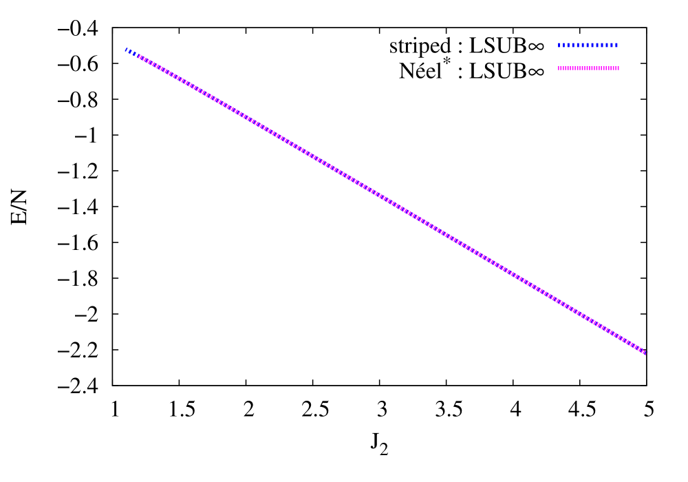
(a) $E/N$

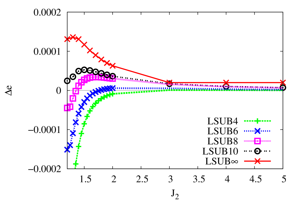
(b) $\Delta e$

Figure 2: (a) The extrapolated CCM LSUB$\infty$ results for the gs energy per spin, $e\equiv E/N$, versus $J_{2}$ for the striped and Néel^∗ phases of the spin-$\frac{1}{2}$ $J_{1}$–$J_{2}$ Heisenberg antiferromagnet on the checkerboard lattice (with $J_{1}=1$), using the LSUB$m$ results with $m=\{4,6,8,10\}$ and Eq. (4); (b) the energy difference, $\Delta e\equiv e^{{\rm striped}}-e^{{\rm N\acute{e}el}^{\ast}}$ versus $J_{2}$ of the two phases shown in (a) using LSUB$m$ approximations with $m=\{4,6,8,10\}$ and also using the corresponding separate LSUB$\infty$ results for both phases from Eq. (4) using $m=\{4,6,8,10\}$.

Thus, as a final step we need to extrapolate the raw CCM data from our LSUB$m$ approximations to the exact ($m\to\infty$) limit. In the absence of any staggering effects of the sort described above, we use the well-tested extrapolation scheme

$$E(m)/N=a_{0}+a_{1}m^{-2}+a_{2}m^{-4}\,,$$ (4)

for the gs energy.Kr:2000 ; ccm3 ; Fa:2001 ; rachid05 ; schmalfuss ; Bi:2008_PRB ; darradi08 ; Bi:2008_JPCM ; richter10 ; Reuther:2011_J1J2J3mod For the magnetic order parameter, $M$, we use the schemes

$$M(m)=b_{0}+b_{1}m^{-1}+b_{2}m^{-2}\,,$$ (5)

for non-frustrated spin systems,Kr:2000 ; ccm3 ; Fa:2001 and

$$M(m)=c_{0}+b_{1}m^{-1/2}+a_{2}m^{-3/2}\,,$$ (6)

for highly frustrated spin systems.darradi08 ; Bi:2008_JPCM ; richter10 ; Reuther:2011_J1J2J3mod We have performed separate extrapolations using data sets with $m=\{4,6,8,10\}$, $m=\{6,8,10\}$, $m=\{2,4,6,8\}$, and $m=\{4,6,8\}$. They yield very similar results in each of the cases reported below, which gives credence to our results and demonstrates their robustness.

IV RESULTS AND DISCUSSION

We now present our CCM results for the spin-$\frac{1}{2}$ anisotropic checkerboard model, using each of the three states shown in Fig. 1 as model states. We first show in Fig. 2(a) the extrapolated LSUB$\infty$ gs energies per spin, $E/N$, of the phases obtained using the striped and Néel^∗ model states. We recall that in the classical limit ($s\rightarrow\infty$) these two phases are degenerate and are the gs phase only for $\kappa>1$. Results are shown in Fig. 2(a) down to the lowest terminating values of $\kappa$ in each case for which real solutions exist for all of the LSUB$m$ approximations used. It has been shown previouslyFa:2004 ; UJack_ccm that such termination points are a strong indication of the corresponding quantum phase transition points that occur in the system under study. Figure 2(b) shows the difference in the energies of the two states in the approximate region where both CCM solutions exist. We see clearly that although the energy difference is small, the classical degeneracy is removed in favor of the Néel^∗ state over the striped state for all values of $\kappa$ for which real CCM solutions for both phases exist. Nevertheless, bearing in mind the smallness of the energy difference, we present some results below using both states as model states.

In Fig. 3 we show both the LSUB$m$ and the extrapolated LSUB$\infty$

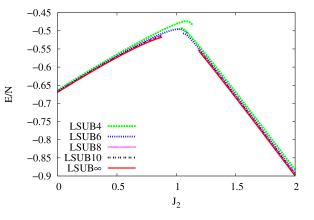
Figure 3: CCM results for the gs energy, $E/N$, for the Néel and Néel^∗ states for the spin-$\frac{1}{2}$ $J_{1}$–$J_{2}$ Heisenberg antiferromagnet on the checkerboard lattice (with $J_{1}=1$) versus $J_{2}$. The LSUB$m$ approximations for $m=\{4,6,8,10\}$ are shown together with the corresponding LSUB$\infty$ extrapolation from using Eq. (4) with $m=\{4,6,8,10\}$.

results for the gs energy, $E/N$, of both the Néel and Néel^∗ phases.

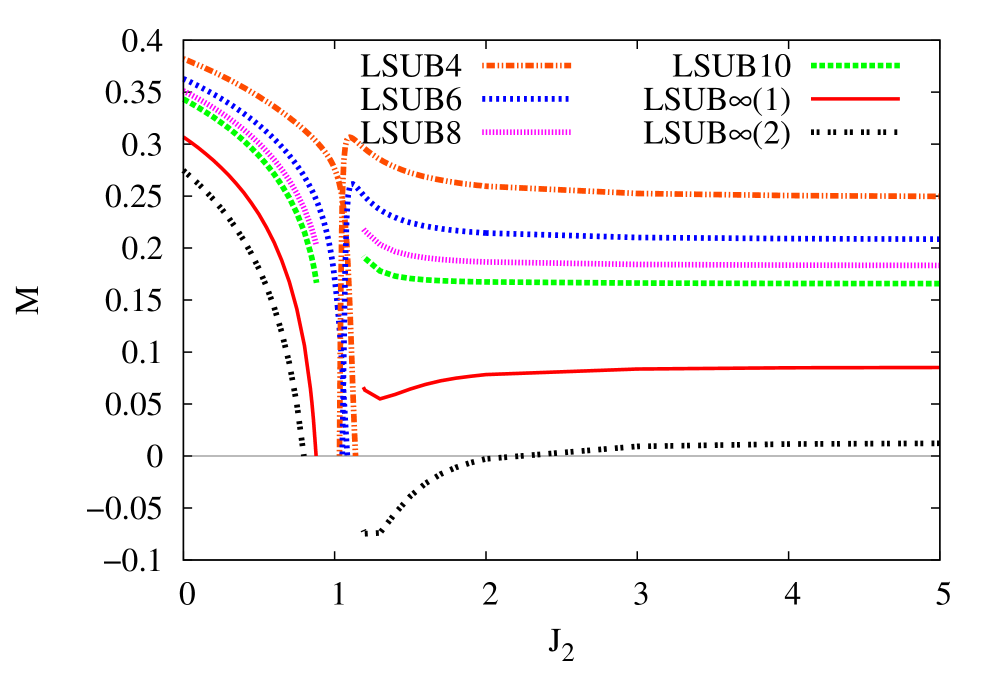
(a) Néel and Néel^∗ states

(b) Néel and striped states

Figure 4: CCM results for the gs magnetic order parameter, $M$, for the Néel and Néel^∗ states for the spin-$\frac{1}{2}$ $J_{1}$–$J_{2}$ Heisenberg antiferromagnet on the checkerboard lattice (with $J_{1}=1$) versus $J_{2}$; (a) using the Néel and Néel^∗ states as model states, and (b) using the Néel and striped states as model states. In both cases the LSUB$m$ approximations for $m=\{4,6,8,10\}$ are shown together with the corresponding LSUB$\infty$(1) and LSUB$\infty$(2) extrapolation from using Eqs. (5) and (6) respectively, with $m=\{4,6,8,10\}$.

As noted briefly above, we now observe more clearly that each of the LSUB$m$ energy curves based on a particular model state terminates at some critical value of $\kappa$ (that itself depends on the LSUB$m$ approximation used), beyond which no real CCM solution can be found. Since the CCM LSUB$m$ solutions require increasingly more computational power to obtain (to a given level of numerical accuracy) as the termination points are approached, it is computationally costly to determine the actual termination points to a high degree of accuracy. We note that in Fig. 3 results are shown for each LSUB$m$ case down to values of $\kappa$ below which for the Néel^∗ phase, and up to values of $\kappa$ above which for the Néel phase, real solutions based on the respective model state cease to exist. As noted above, in all cases the corresponding termination point at a given LSUB$m$ level shown in Fig. 2 for the striped state is lower than that for the equivalent Néel^∗ model state case.

We note however that, as is usually the case, the CCM LSUB$m$ results for finite $m$ values for both the Néel and Néel^∗ phases shown in Fig. 3 extend beyond the corresponding LSUB$\infty$ transition points. For large values of $m$ the LSUB$m$ transition points are quite close to the actual quantum critical points (QCPs) where that phase ends. For example, the LSUB10 termination points shown in Fig. 3 are at $\kappa^{{\rm N\acute{e}el}}_{t}\approx 0.88$ for the Néel state and $\kappa^{{\rm N\acute{e}el}^{\ast}}_{t}\approx 1.2$ for the Néel^∗ state. The CCM results show a clear intermediate regime in which neither of the quasiclassical AFM states (Néel and Néel^∗) is stable.

We now discuss the magnetic order parameter (viz., the average on-site magnetization), $M$, in order to investigate the stability of the quasiclassical magnetic LRO. Our CCM results for $M$ are shown in Fig. 4 for each of the Néel, Néel^∗, and striped phases. Our extrapolated results for $M$ in the Néel phase are seen to be somewhat sensitive to whether we use the scheme of Eq. (5) or that of Eq. (6). As we have indicated previously the scheme of Eq. (5) is appropriate only for small values of $J_{2}$. For example, in the square-lattice limit, $J_{2}=0$, we obtain the extrapolated LSUB$\infty$(1) result $M\approx 0.3069$ from the use of Eq. (5) and the LSUB$m$ values with $m=\{4,6,8,10\}$. Very similar values are obtained with the alternative data sets $m=\{4,6,8\}$ and $m=\{6,8,10\}$. We note that for the square-lattice HAFM no dynamic (or geometric) frustration exists and the Marshall-Peierls sign ruleMarshall-Peierls applies and may hence be used to circumvent the QMC “minus-sign problem.” The QMC result,Sandvik:1997 $M=0.3070\pm 0.0003$, is thus extremely accurate for this limiting ($J_{2}=0$) case only. Our own CCM result using the scheme of Eq. (5) is thus in excellent agreement with it. By contrast, the extrapolation scheme of Eq. (6), which is appropriate for (highly) frustrated systems, gives a much poorer estimate of $M\approx 0.275$.

The magnetization results show clear evidence for the melting of Néel order at a value $\kappa=\kappa_{c_{1}}<\kappa_{{\rm cl}}=1$, with results for $\kappa_{c_{1}}$ that are very close to the corresponding termination point $\kappa^{\rm N\acute{e}el}_{t}$ discussed above. At such values $\kappa\lesssim 1$, where the system is highly frustrated, the extrapolation scheme of Eq. (6) is more appropriate, as we have indicated previously, and its use with the LSUB$m$ data set $m=\{4,6,8,10\}$ gives us our first estimate for the quantum critical point (QCP) at which Néel order vanishes, $\kappa_{c_{1}}\approx 0.796$. Very similar results are found by using the alternative data sets $m=\{4,6,8\}$ and $m=\{6,8,10\}$. Combining all these results gives the estimate $\kappa_{c_{1}}\approx 0.80\pm 0.01$. (By contrast, the use of the scheme of Eq. (5), which is inappropriate in this frustrated region near a QCP, gives a value $\kappa_{c_{1}}\approx 0.87\pm 0.01$.)

The results in Fig. 4(a) for $M$ using the Néel^∗ state as CCM model state are seen to be qualitatively very different from those using the Néel state as model state. Indeed, all of the evidence from Fig. 4(a) is that $M$ is either zero or very close to zero over the entire range for which CCM extrapolated LSUB$\infty$ solutions exist using the Néel^∗ state as model state. The more appropriate extrapolation scheme of Eq. (6) in this regime with $\kappa\gtrsim 1$ gives either negative values for $M$ or positive values very close to zero over the entire range shown in Fig. 4, while even the inappropriate scheme of Eq. (5) gives only a very small and almost constant value of $M\approx 0.08$ over the same range. Our results in the high-frustration regime ($\kappa\gg 1$) using the appropriate scheme of Eq. (6) are given extra credence by the fact that we see clearly from Fig. 4 that $M\rightarrow 0$ rather accurately in the large $\kappa$ limit, which is the exact result for this limit where the model reduces to unlinked 1D spin-$\frac{1}{2}$ chains. It is clear that at best the existence of the Néel^∗ phase in the spin-$\frac{1}{2}$ case is extremely fragile from this evidence. More likely, it is not the stable gs phase for any value of $\kappa$, based on the results for $M$.

For this reason we have repeated the calculations for $M$, but now using the striped state as CCM model state, even though we found it to have a slightly higher energy for all values of $\kappa$ than that of the Néel^∗ state. Results are shown in Fig. 4(b). Figures 4(a) and 4(b) show very similar results for $M$ for the striped state and the Néel^∗ state, except very near their corresponding termination points. All of the evidence so far is that neither state is the stable gs phase for any value of $\kappa$. Since the results for the order parameter $M$ are so similar for the Néel^∗ state and the striped state, and since the former has a slightly lower energy, we henceforth restrict ourselves for larger values of $\kappa$ to use of the Néel^∗ state as CCM model state.

It is reasonably well established from earlier numerical studies using EDFouet:2003 and strong-coupling expansion techniquesBerg:2003 ; Brenig:2002 ; Brenig:2004 that the gs phase of the spin-$\frac{1}{2}$ HAFM on the checkerboard lattice (i.e., our model at the isotropic point $J_{2}=J_{1}$) is a plaquette valence-bond crystal (PVBC) with long-range quadrumer order. Further evidence for such a valence-bond solid built from disconnected 4-spin singlets comes from a “fermionic” SU($n$) generalization of the SU(2) group in the large-$n$ limit.Canals:2002 There is broad agreement from all this work that the PVBC phase comprises singlet plaquettes on the squares in Fig. 1 without crossed links, as shown in Fig. 5.

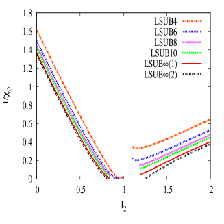
(a)

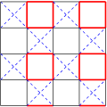
(b)

Figure 5: (Color online) Left: CCM results for the inverse plaquette susceptibility, $1/\chi_{p}$, versus $J_{2}$, using the Néel and Néel^∗ states as model states, for the spin-$\frac{1}{2}$ $J_{1}$–$J_{2}$ Heisenberg antiferromagnet on the checkerboard lattice (with $J_{1}=1$). The LSUB$m$ approximations for $m=\{4,6,8,10\}$ are shown together with the corresponding LSUB$\infty$(1) and LSUB$\infty$(2) results from using the extrapolations schemes of Eqs. (7) and (8) respectively, with $m=\{4,6,8,10\}$. Right: The perturbations (fields) $F=\delta\,\hat{O}_{p}$ for the plaquette susceptibility $\chi_{p}$. Thick (red) and thin (black) lines correspond respectively to strengthened and weakened NN exchange couplings, where $\hat{O}_{p}=\sum_{\langle i,j\rangle}a_{ij}\mathbf{s}_{i}\cdot\mathbf{s}_{j}$, and the sum runs over all NN bonds, with $a_{ij}=+1$ and $-1$ for thick (red) and thin (black) lines respectively.

Thus, in order to get more information on the phase that occurs after the melting of Néel order at $\kappa=\kappa_{c_{1}}$ we now investigate the possibility that it might be a PVBC state of the sort shown in Fig. 5.

To do so we first consider a generalized susceptibility $\chi_{F}$ that describes the response of the system to a perturbation described by a “field” operator $F$. A field term $F=\delta\,\hat{O}_{F}$ is thus added to the Hamiltonian of Eq. (1). The energy per site in a given state, $E(\delta)/N\equiv e(\delta)$, is then calculated for the perturbed Hamiltonian $H+F$, and the susceptibility of the system to the perturbation $F$ is defined as $\chi_{F}\equiv-\left.(\partial^{2}{e(\delta)})/(\partial{\delta}^{2})\right|_{\delta=0}$. An instability of the state against the perturbation $F$ is signalled by a zero point of $\chi_{F}^{-1}$ or, equivalently, by a divergence of $\chi_{F}$. In our case we first use the CCM to calculate $\chi_{F}$, using a specific model state, in various LSUB$m$ approximations. Although rather less empirical experience is available for the $m\to\infty$ extrapolation of the CCM data for $\chi_{F}$ than for other quantities such as the gs energy $E$ or the order parameter $M$, we have found previouslyFarnell:2011 that the same extrapolation used for the gs energy [i.e., $\chi_{F}(m)=d_{0}+d_{1}m^{-2}+d_{2}m^{-4}$] fits the data most accurately, at least in regions not too close to a divergence of the susceptibility. We also saw previouslyFarnell:2011 that a corresponding extrapolation of the inverse susceptibility,

$$\chi_{F}^{-1}(m)=x_{0}+x_{1}m^{-2}+x_{2}m^{-4}\,,$$ (7)

gave very consistent results that agreed very closely with those from the corresponding above extrapolation of $\chi_{F}$, except again in regions close to where $\chi_{F}^{-1}\to 0$. Since, as we will see below, we will be especially interested in precisely such regions over a large range of values of $\kappa$, we also use the fitting function,

$$\chi_{F}^{-1}(m)=y_{0}+y_{1}m^{-y_{2}}\,.$$ (8)

To calculate the susceptibility, $\chi_{p}$, of our system against PVBC ordering we thus set the operator $\hat{O}_{F}$ to $\hat{O}_{p}$ as illustrated in the right panel and the caption of Fig. 5. The perturbation field $F$ thus breaks the translational symmetry of $H$. We show CCM results in the left panel of Fig. 5 using both the Néel and Néel^∗ states as model states. We first observe that for smaller values of $J_{2}$ (i.e., on the Néel side) the two extrapolations agree very closely, even near the point at which $\chi_{p}^{-1}$ goes to zero. Thus, the extrapolated inverse plaquette susceptibility using the LSUB$m$ data set $m=\{4,6,8,10\}$ ($m=\{6,8,10\}$) vanishes on the Néel side at $\kappa\approx 0.843$ ($\kappa\approx 0.833$) using the extrapolation scheme of Eq. (7), and at $\kappa\approx 0.820$ ($\kappa\approx 0.775$) using the extrapolation scheme of Eq. (8). Since the exponent $y_{2}$ in Eq. (8) falls rather sharply to a value close to 1 near the point at which $\chi_{p}^{-1}$ vanishes, the best estimate for this point is more likely to come from the extrapolation scheme of Eq. (8) than from that of Eq. (7).

Combining all these results gives our best estimate of $\kappa\approx 0.79\pm 0.03$ for the point at which the Néel phase becomes susceptible to PVBC ordering. This is in very good agreement with the above estimate of $\kappa_{c_{1}}\approx 0.80\pm 0.01$ at which Néel LRO disappears as measured by our results for the order parameter $M$. Thus, our results show no evidence at all for a coexistence region in which Néel and PVBC ordering are both present, such as has been suggested might occur,Sachdev:2002 although we cannot exclude the possibility of a very narrow region of coexistence confined to the region $0.79\lesssim\kappa\lesssim 0.81$. Our findings are in agreement with ED resultsSindzingre:2002 for the same spin-$\frac{1}{2}$ anisotropic planar pyrochlore model that reach the conclusion that, if present at all, any such coexistence region is very narrow indeed. As has been discussed in detail elsewhere,Starykh:2005 the QCP at $\kappa_{c_{1}}$ between the Néel and PVBC phases is both forbidden as a continuous transition within standard Landau-Ginzburg theory and does not seem either to be a viable candidate for a deconfined (continuous) transition. The shape of the magnetization curves in Fig. 4 on the Néel side, which show a rapid decrease near $\kappa_{c_{1}}$, is perhaps more indicative of a first-order transition, as we have observed previously,Farnell:2011 although such evidence should not be regarded as conclusive.

We also observe from Fig. 5 that with the Néel^∗ state used as our CCM model state the two extrapolations of Eqs. (7) and (8) for the inverse plaquette susceptibility, $\chi_{p}^{-1}$, agree quite closely at larger values of $\kappa$ but diverge slightly at smaller values, where $\chi_{p}^{-1}$ itself becomes small. As $\kappa\to\infty$ we observe that the exponent $y_{2}$ in Eq. (8) appears to approach the value 1.5 [rather than 2 as in Eq. (7)], and then drop to a value close to 1 as $\chi_{p}^{-1}$ approaches zero. For these reasons again, we expect the extrapolation of Eq. (8) to be more exact, especially in regions where $\chi_{p}^{-1}$ becomes small. Thus, the extrapolated inverse plaquette susceptibility using the LSUB$m$ data set $m=\{4,6,8,10\}$ ($m=\{6,8,10\}$) vanishes on the Néel^∗ side at $\kappa\approx 1.238$ ($\kappa\approx 1.216$) using the extrapolation scheme of Eq. (8). Although, as we have seen, the Néel^∗ state does not appear to exist as as a stable gs phase (since its order parameter $M$ seems to vanish for all values of $\kappa$, nevertheless the results using it as a CCM model state provide a robust basis for the calculation of $\chi_{p}$, and give an estimate $\kappa_{c_{2}}\approx 1.22\pm 0.02$ for the upper QCP at which PVBC order disappears.

However, we are now led to the question of what is the actual gs phase of the model for larger values of frustration, $\kappa>\kappa_{c_{2}}$, beyond the upper QCP (at $\kappa=\kappa_{c_{2}}$) at which the PVBC phase ceases to exist as a stable gs phase. In the first place it is clear that such a QCP must exist since in the limit $\kappa\rightarrow\infty$ one has the physics of decoupled HAFM 1D chains, which are known to exhibit Luttinger spin-liquid behavior, and are typified by a gapless excitation spectrum and spin-spin correlations that decay algebraically with inter-spin separation distance. It was arguedStarykh:2002 that for large values of $\kappa$, where the 1D chains are weakly coupled, the gs phase might be a 2D sliding Luttinger liquid phase (characterized by the absence of LRO and with massless deconfined spinons as the elementary excitations) that joined smoothly to the $\kappa\to\infty$ limit. It was later shown,Starykh:2005 by a more careful analysis of the relevant terms near the Luttinger liquid fixed point of the independent 1D spin chain, that this finding was incorrect. Instead, using techniques that combine renormalization group ideas and 1D bosonization and current algebra methods, it was shown that in this large-$\kappa$ regime the gs phase is of spontaneously dimerized type, with a staggered ordering of dimers along the parallel chains (viz., the diagonals in Fig. 1). Such a crossed-dimer valence-bond crystal (CDVBC) phase, with twofold spontaneous symmetry breaking and no magnetic order, was independently confirmedArlego:2007 by a series expansion (SE) technique based on the flow equation method.

The CDVBC phase is illustrated in the right panel of Fig. 6. Similarly

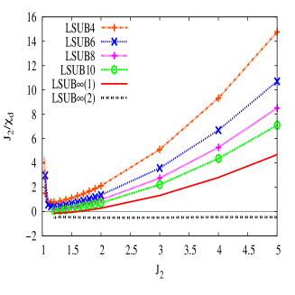
(a)

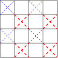
(b)

Figure 6: (Color online) Left: CCM results for the scaled inverse crossed dimer susceptibility, $J_{2}/\chi_{d}$, using the Néel^∗ state as model state, for the spin-$\frac{1}{2}$ $J_{1}$–$J_{2}$ Heisenberg antiferromagnet on the checkerboard lattice (with $J_{1}=1$) versus $J_{2}$. The LSUB$m$ approximations for $m=\{4,6,8,10\}$ are shown together with the corresponding LSUB$\infty$(1) and LSUB$\infty$(2) results from using the extrapolations schemes of Eqs. (7) and (8) respectively, with $m=\{4,6,8,10\}$. Right: The perturbations (fields) $F=\delta\,\hat{O}_{d}$ for the dimer susceptibility $\chi_{d}$. Thick (red) dashed and thin (blue) dashed lines correspond respectively to strengthened and weakened NNN exchange couplings, where $\hat{O}_{d}=\sum_{\langle\langle i,k\rangle\rangle}a_{ik}\mathbf{s}_{i}\cdot\mathbf{s}_{k}$, and the sum runs over the NNN diagonal bonds of the checkerboard lattice, with $a_{ik}=+1$ and $-1$ for thick (red) dashed and thin (blue) dashed lines respectively.

to what was done above for the PVBC susceptibility, $\chi_{p}$, we can now calculate the susceptibility, $\chi_{d}$ of our system against CDVBC ordering by setting the perturbation operator $\hat{O}_{F}$ to the operator $\hat{O}_{d}$ illustrated in the right panel and the caption of Fig. 6. Since in the large $J_{2}$ limit the energy scales linearly with $J_{2}$ (as may clearly also be observed from Figs. 2(a) and 3, we show our CCM results in Fig. 6 for the scaled inverse dimer susceptibility, $J_{2}/\chi_{d}$ as a function of $J_{2}$.

Interestingly, in this case, the extrapolation scheme of Eq. (7) does not fit the LSUB$m$ data points at all well, and consequently gives a very poor fit. The reason becomes quite evident when the extrapolation scheme of Eq. (8) is used instead. It is then observed that that the scaling exponent $y_{2}$ approaches the value 0.75 for large values of $J_{2}$, and even for smaller values near the QCP at $\kappa=\kappa_{c_{2}}$ only rises slightly to values that approach 1. It is clear that the extrapolated value of $J_{2}/\chi_{d}$ is small, slightly negative, and almost constant for all values of $\kappa$ shown, when the more flexible extrapolation scheme of Eq. (8) is used. Our results are consistent with the interpretation that the inverse dimer susceptibility is zero for all values $\kappa$ shown in Fig. 6, namely those where we have real solutions to the equations pertaining to all of the CCM LSUB$m$ schemes used. The actual lower termination point is not easy to determine accurately in this way, as we have already mentioned above. However, it is quite clear from Fig. 6 that the individual LSUB$m$ curves all have a minimum at a value $\kappa\approx 1.20\pm 0.05$, and our results are thus consistent with the interpretation that the inverse dimer susceptibility is zero for all values $\kappa>\kappa_{c_{2}}$. In that scenario there is a QCP between the PVBC and CDVBC phases at $\kappa=\kappa_{c_{2}}$, and the CDVBC phase then persists out to the $\kappa\to\infty$ limit of unlinked 1D chains, which is itself a singular point.

Our results give us essentially no information, however, on the nature of the transition at $\kappa_{c_{2}}$. Starykh et al.Starykh:2005 have concluded that a continuous transition between the PVBC and CDVBC phases is prohibited within the standard Landau-Ginzburg scenario of phase transitions. They argue further that the most probable alternative is a direct first-order transition, although a separate possibility is again the existence of an intermediate coexistence phase with both valence-bond orderings that can then have separate continuous transitions to both the PVBC and CDVBC phases. From our results we clearly favor the former scenario, although we cannot exclude the possibility of a very narrow such coexistence phase confined to the region $1.20\lesssim\kappa\lesssim 1.22$.

V SUMMARY AND CONCLUSIONS

To summarize, we have investigated the gs properties and ($T=0$) phase diagram of the frustrated spin-$\frac{1}{2}$ antiferromagnetic $J_{1}$–$J_{2}$ model (with $J_{2}\equiv\kappa J_{1}\,;J_{1}>0)$ on the 2D checkerboard lattice, using the CCM carried out to high orders.

In common with most other calculations on the model we find that the gs phase is an AFM Néel-ordered state for $\kappa<\kappa_{c_{1}}$, at which point the staggered Néel magnetization vanishes. Our best estimate for this lower QCP is $\kappa_{c_{1}}\approx 0.80\pm 0.01$. This is in reasonable agreement, but probably more accurate than, a corresponding estimate of $\kappa_{c_{1}}\approx 0.75$ from an ED studySindzingre:2002 on samples of $N=16,32,36$ spins. Since we calculate that the Néel-ordered state becomes susceptible to PVBC ordering at $\kappa\approx 0.79\pm 0.03$ our results point then to a direct transition from the Néel-ordered gs phase to a PVBC phase at $\kappa=\kappa_{c_{1}}$, although we cannot exclude entirely the small possibility of a vey narrow coexistence region. This finding is in good agreement with that found from ED studies.Sindzingre:2002 We estimate that any such coexistence region of AFM Néel ordering and quadrumer plaquette ordering is confined to the parameter range $0.79\lesssim\kappa\lesssim 0.81$. Our estimate for the lower boundary at which the quadrumer PVBC ordering vanishes is in excellent agreement with the corresponding value $\kappa\approx 0.80\pm 0.01$ from a high order SE calculationBrenig:2004 that starts from the limit of uncoupled quadrumers. A recent tensor network simulation of the modelChan:2011 gives a somewhat higher value of $\kappa_{c_{1}}\approx 0.88$ for the QCP from the Néel gs phase to the PVBC gs phase.

From our CCM calculations we estimate that the quadrumer order of the PVBC state vanishes at a higher QCP at $\kappa=\kappa_{c_{2}}\approx 1.22\pm 0.02$. This is in reasonable agreement, although somewhat higher than the corresponding estimates $\kappa\approx 1.095\pm 0.035$ from a high-order SE calculation,Brenig:2004 and $\kappa\approx 1.11$ from a tensor network simulation.Chan:2011

Although the striped and Néel^∗ states, which are the fourfold-degenerate quasiclassical gs phases at $O(1/s)$ in an expansion in powers of $1/s$ for $\kappa>1$,Tchernyshyov:2003 provide excellent model states for CCM calculations at larger values of $\kappa\gtrsim 1$ in the sense of providing well-converged LSUB$m$ results, we find that they are not stable gs phases for the spin-$\frac{1}{2}$ model for any value of $\kappa$. This is in sharp disagreement with the finding from a recent tensor network simulationChan:2011 that the striped and/or Néel^∗ states form the stable gs phase for all values $\kappa>\kappa_{c_{2}}$. By contrast we find from our CCM calculations that the Néel^∗ state is susceptible to the formation of a CDVBC phase (with an inverse susceptibility that is essentially zero) for all values $\kappa\gtrsim 1.20\pm 0.05$. We conclude that the CDVBC state is thus likely to be the stable gs phase for $\kappa>\kappa_{c_{2}}$, although we cannot exclude the possibility of a very narrow coexistence regime confined to the range $1.20\lesssim\kappa\lesssim 1.22$. We find no evidence at all for any region separating the PVBC and CDVBC phases where the Néel^∗ state would form a stable gs phase, thereby ruling out one of the two scenarios postulated by Starykh et al.,Starykh:2005 although now in complete agreement with their other scenario for the gs phase diagram, on which we now provide accurate numerical results for the two QCP’s at $\kappa_{c_{1}}$ and $\kappa_{c_{2}}$.

Finally we note that the CCM has been used here with the model or reference states chosen as classical states built from independent-spin product states. For larger values of the frustration parameter, $\kappa>\kappa_{c_{1}}$, we remark that these model states are able (with appropriate choice of additional perturbative terms in the Hamiltonian), to describe the susceptibilities of the system to form the true gs phasaes perfectly well, even though we have shown that the respective extrapolated order parameters with respect to these model states are essentially zero over the entire range. Nevertheless, it would be worthwhile to repeat the CCM calculations directly with dimer and plaquette valence-bond states. Indeed, just such a general CCM approachFarnell_VBgroundstates:2009 has recently been described, which combines exact solutions for dimer or plaquette valence-bond solid ground states with the computational implementation described hereccm that is based on independent-spin product model states. It would be interesting to use this formalism for the present model in order to confirm our results.

References

- (1) S. Sachdev, in Low Dimensional Quantum Field Theories for Condensed Matter Physicists, edited by Y. Lu, S. Lundqvist, and G. Morandi (World Scientific, Singapore, 1995).
- (2) Quantum Magnetism, Lecture Notes in Physics 645 edited by U. Schollwöck, J. Richter, D. J. J. Farnell, and R. F. Bishop (Springer-Verlag, Berlin, 2004).
- (3) G. Misguich and C. Lhuillier, in Frustrated Spin Systems, edited by H.T. Diep (World Scientific, Singapore, 2005), p. 229.
- (4) J. Struck, C. Ölschäger, R. Le Targat, P. Soltan-Panahi, A. Eckardt, M. Lewenstein, P. Windpassinger, and K. Sengstock, Science 333, 996 (2011).
- (5) H. Fukuzawa, D. Yanagishima, R. Higashinaka, and Y. Maeno, Acta Phys. Pol. B 34, 1501 (2003).
- (6) R. R. P. Singh, O. A. Starykh, and P. J. Freitas, J. Appl. Phys. 83, 7387 (1998).
- (7) S. E. Palmer and J. T. Chalker, Phys. Rev. B 64, 094412 (2001).
- (8) C. H. Chung, J. B. Marston, and S. Sachdev, Phys. Rev. B 64, 134407 (2001).
- (9) W. Brenig and A. Honecker, Phys. Rev. B 65, 140407(R) (2002).
- (10) B. Canals, Phys. Rev. B 65, 184408 (2002).
- (11) O. A. Starykh, R. R. P. Singh, and G. C. Levine, Phys. Rev. Lett. 88, 167203 (2002).
- (12) P. Sindzingre, J.-B. Fouet, and C. Lhuillier, Phys. Rev. B 66, 174424 (2002).
- (13) J.-B. Fouet, M. Mambrini, P. Sindzingre, and C. Lhuillier, Phys. Rev. B 67, 054411 (2003).
- (14) E. Berg, E. Altman, and A. Auerbach, Phys. Rev. Lett. 90, 147204 (2003).
- (15) O. Tchernyshyov, O. A. Starykh, R. Moessner, and A. G. Abanov, Phys. Rev. B 68, 144422 (2003).
- (16) R. Moessner, O. Tchernyshyov, and S. L. Sondhi, J. Stat. Phys. 116, 755 (2004).
- (17) M. Hermele, M. P. A. Fisher, and L. Balents, Phys. Rev. B 69, 064404 (2004).
- (18) W. Brenig and M. Grzeschik, Phys. Rev. B 69, 064420 (2004).
- (19) J. S. Bernier, C. H. Chung, Y. B. Kim, and S. Sachdev, Phys. Rev. B 69, 214427 (2004).
- (20) O. A. Starykh, A. Furusaki, and L. Balents, Phys. Rev. B 72, 094416 (2005).
- (21) H.-J. Schmidt, J. Richter, and R. Moessner, J. Phys. A: Math. Gen. 39, 10673 (2006).
- (22) M. Arlego and W. Brenig, Phys. Rev. B 75, 024409 (2007); ibid. 80, 099902(E) (2009).
- (23) S. Moukouri, Phys. Rev. B 77, 052408 (2008).
- (24) Y.-H. Chan, Y.-J. Han, and L.-M. Duan, Phys. Rev. B 84, 224407 (2011).
- (25) F. Wegner, Ann. Phys. (Leipzig) 3, 77 (1974).
- (26) C. J. Morningstar and M. Weinstein, Phys. Rev. D 54, 4131 (1996).
- (27) J. Jordan, R. Orús, G. Vidal, F. Verstraete, and J. I. Cirac, Phys. Rev. Lett. 101, 250602 (2008).
- (28) R. F. Bishop, Theor. Chim. Acta 80, 95 (1991).
- (29) R. F. Bishop, in Microscopic Quantum Many-Body Theories and Their Applications, Lecture Notes in Physics Vol. 510, edited by J. Navarro and A. Polls, (Springer-Verlag, Berlin, 1998), p. 1.
- (30) D. J. J. Farnell and R. F. Bishop, in Quantum Magnetism, Lecture Notes in Physics Vol. 645, edited by U. Schollwöck, J. Richter, D. J. J. Farnell, and R. F. Bishop, (Springer-Verlag, Berlin, 2004), p. 307.
- (31) C. Zeng, D. J. J. Farnell, and R. F. Bishop, J. Stat. Phys. 90, 327 (1998).
- (32) S. E. Krüger, J. Richter, J. Schulenburg, D. J. J. Farnell, and R. F. Bishop, Phys. Rev. B 61, 14607 (2000).
- (33) R. F. Bishop, D. J. J. Farnell, S.E. Krüger, J. B. Parkinson, J. Richter, and C. Zeng, J. Phys.: Condens. Matter 12, 6887 (2000).
- (34) D. J. J. Farnell, R. F. Bishop, and K. A. Gernoth, Phys. Rev. B 63, 220402(R) (2001).
- (35) R. Darradi, J. Richter, and D. J. J. Farnell, Phys. Rev. B 72, 104425 (2005).
- (36) D. Schmalfuß, R. Darradi, J. Richter, J. Schulenburg, and D. Ihle, Phys. Rev. Lett. 97, 157201 (2006).
- (37) R. Darradi, O. Derzhko, R. Zinke, J. Schulenburg, S. E. Krüger, and J. Richter, Phys. Rev. B 78, 214415 (2008).
- (38) R. F. Bishop, P. H. Y. Li, R. Darradi, and J. Richter, J. Phys.: Condens. Matter 20, 255251 (2008).
- (39) R. F. Bishop, P. H. Y. Li, R. Darradi, J. Schulenburg, and J. Richter, Phys. Rev. B 78, 054412 (2008).
- (40) J. Richter, R. Darradi, J. Schulenburg, D.J.J. Farnell, and H. Rosner, Phys. Rev. B 81, 174429 (2010).
- (41) R. F. Bishop, P. H. Y. Li, D. J. J. Farnell, and C. E. Campbell, Phys. Rev. B 82, 024416 (2010).
- (42) J. Reuther, P. Wölfle, R. Darradi, W. Brenig, M. Arlego, and J. Richter, Phys. Rev. B 83, 064416 (2011).
- (43) D. J. J. Farnell, R. F. Bishop, P. H. Y. Li, J. Richter, and C. E. Campbell, Phys. Rev. B 84, 012403 (2011).
- (44) O. Götze, D. J. J. Farnell, R. F. Bishop, P. H. Y. Li, and J. Richter, Phys. Rev. B 84, 224428 (2011).
- (45) S. Sachdev and K. Park, Ann. Phys. (N.Y.) 298, 58 (2002).
- (46) V. J. Emery, E. Fradkin, S. A. Kivelson, and T. C. Lubensky, Phys. Rev. Lett. 85, 2160 (2000).
- (47) R. Mukhopadhyay, C. L. Kane, and T. C. Lubensky, Phys. Rev. B 64, 045120 (2001).
- (48) A. Vishwanath and D. Carpentier, Phys. Rev. Lett. 86, 676 (2001).
- (49) J. Villain, J. Phys. (France) 38, 385 (1977); J. Villain, R. Bidaux, J. P. Carton, and R. Conte, ibid. 41, 1263 (1980).
- (50) We use the program package CCCM of D. J. J. Farnell and J. Schulenburg, see http://www-e.uni-magdeburg.de/jschulen/ccm/index.html.
- (51) D. J. J. Farnell and R. F. Bishop, Int. J. Mod. Phys. B 20, 3369 (2008).
- (52) W. Marshall, Proc. R. Soc. London, Ser. A 232, 48 (1955).
- (53) A. W. Sandvik, Phys. Rev. B 56, 11678 (1997).
- (54) D. J. J. Farnell, J. Richter, R. Zinke, and R. F. Bishop, J. Stat. Phys. 135, 175 (2009).