Spitzer/MIPS 24 µm Observations of HD 209458b: 3 Eclipses, 2.5 Transits, and a Phase Curve Corrupted by Instrumental Sensitivity Variations.

Abstract

We report the results of an analysis of all Spitzer/MIPS 24 µm observations of HD 209458b, one of the touchstone objects in the study of irradiated giant planet atmospheres. Altogether we analyze two and a half transits, three eclipses, and a 58-hour near-continuous observation designed to detect the planet’s thermal phase curve. The results of our analysis are: (1) A mean transit depth of $1.484\%\pm 0.033\%$, consistent with previous measurements and showing no evidence of variability in transit depth at the 3% level. (2) A mean eclipse depth of $0.338\%\pm 0.026\%$, somewhat higher than that previously reported for this system; this new value brings observations into better agreement with models. From this eclipse depth we estimate an average dayside brightness temperature of $1320\textrm{~{}K}\pm 80\textrm{~{}K}$; the dayside flux shows no evidence of variability at the 12% level. (3) Eclipses in the system occur $32\pm 129\textrm{~{}s}$ earlier than would be expected from a circular orbit, which constrains the orbital quantity $e\cos\omega$ to be $0.00004\pm 0.00033$. This result is fully consistent with a circular orbit and sets an upper limit of 140 m s^-1 ($3\sigma$) on any eccentricity-induced velocity offset during transit. The phase curve observations (including one of the transits) exhibits an anomalous trend similar to the detector ramp seen in previous Spitzer/IRAC observations; by modeling this ramp we recover the system parameters for this transit. The long-duration photometry which follows the ramp and transit exhibits a gradual $\sim 0.2\%$ decrease in flux over $\sim 30$ hr. This effect is similar to that seen in pre-launch calibration data taken with the 24 µm array and is better fit by an instrumental model than a model invoking planetary emission. The large uncertainties associated with this poorly-understood, likely instrumental effect prevent us from usefully constraining the planet’s thermal phase curve. Our observations highlight the need for a thorough understanding of detector-related instrumental effects on long time scales when making the high-precision mid-infrared measurements planned for future missions such as EChO, SPICA, and JWST.

1. Introduction

Most known extrasolar planets were discovered via the radial velocity technique – in which the Doppler wobble of a star indicates an orbiting planet – and/or by the transit method – in which periodic dimming of a star indicates a planet that crosses in front of the stellar disk. Owing to the observational biases of these techniques, the first planets thus discovered were the large, massive objects on few-day orbits commonly known as hot Jupiters (Mayor & Queloz, 1995; Henry et al., 2000; Charbonneau et al., 2000). Their large sizes and high temperatures make these objects excellent candidates for the study of their dayside emission when the planet is occulted by the star (Deming et al., 2005; Charbonneau et al., 2005), of their longitudinally-averaged global emission (Harrington et al., 2006; Cowan et al., 2007; Knutson et al., 2007), and of their atmospheric opacity via the wavelength-dependent flux diminution during transit (Seager & Sasselov, 2000; Charbonneau et al., 2002). These observations have led to measurements of atmospheric abundances of key molecular species (Madhusudhan et al., 2011a), possible non-equilibrium chemistry (Stevenson et al., 2010), high-altitude hazes (Sing et al., 2009), and atmospheric circulation (Cowan & Agol, 2011b).

Any discussion of hot Jupiter atmospheres must necessarily mention two systems in particular. One, HD 189733, is the brightest star known to host a hot Jupiter (Bouchy et al., 2005). The other is HD 209458, the first known transiting planet (Charbonneau et al., 2000; Henry et al., 2000) and the focus of this study. These are the two touchstone objects in the study of irradiated giant exoplanets, both because they were discovered relatively early on and because they orbit especially bright (as seen from Earth) host stars. This last point in particular allows for especially precise characterization of these planets’ atmospheres and permits observations which would provide unacceptably low signal to noise ratios for fainter systems.

1.1. The HD 209458 system

The star HD 209458 is an F8 star roughly 15 % more massive than the Sun (Mazeh et al., 2000; Brown et al., 2001; Baines et al., 2008), with an equivalent metallicity and slightly higher temperature (Schuler et al., 2011). It is orbited by HD 209458b, a roughly 1.4 $R_{J}$, 0.7 $M_{J}$ planet in a 3.5-day, near-circular orbit (Southworth, 2008; Torres et al., 2008). The planet’s parameters have been substantially improved upon since its initial discovery (Charbonneau et al., 2000; Henry et al., 2000; Mazeh et al., 2000). Two sets of more recent values (Torres et al., 2008; Southworth, 2008) do not differ significantly, and we use the former’s system parameters in our analysis when not making our own measurements.

Infrared photometry during eclipses of HD 209458b measured from the ground (Richardson et al., 2003) and with Spitzer (Deming et al., 2005; Knutson et al., 2008) determines the planet’s intrinsic emission spectrum, and is best fit by atmospheric models in which the planet’s atmospheric temperature increases above $\sim 0.1-1$ bar (Burrows et al., 2007, 2008; Fortney et al., 2008; Madhusudhan & Seager, 2010). Such temperature inversions are common on hot Jupiters, and a popular explanation requires the presence of a high-altitude absorber (e.g., Fortney et al., 2008; Burrows et al., 2008). The nature of any such absorber is currently unknown and the subject remains a topic of active research (Désert et al., 2008; Spiegel et al., 2009; Knutson et al., 2010; Madhusudhan et al., 2011b).

If present, a high-altitude optical absorber is expected to absorb the incident stellar flux high in the atmosphere where radiative timescales are short and advection is inefficient (Cowan & Agol, 2011a). Consequently, such planets are expected to exhibit large day/night temperature contrasts and low global energy redistribution despite circulation models’ ubiquitous predictions of large-scale superrotating jets on these planets (Showman & Guillot, 2002; Cooper & Showman, 2005; Cho et al., 2008; Rauscher et al., 2008; Showman et al., 2009; Dobbs-Dixon et al., 2010; Burrows et al., 2010; Rauscher & Menou, 2010; Thrastarson & Y-K. Cho, 2010; Heng et al., 2011b, a). Spitzer/IRAC observations of HD 209458b at 8 µm place an upper limit on the planet’s thermal phase variation of 0.0022 ($3\sigma$; Cowan et al., 2007). Given the planet’s demonstrably low albedo (Rowe et al., 2008) this limit is substantially lower expected if the planet has a low recirculation efficiency. In hot Jupiter atmospheres the dominant 24 µm molecular opacity source is expected to be $\textrm{H}_{2}\textrm{O}$, but there is some tension between models and past observations at this wavelength (cf. Madhusudhan & Seager, 2010). Thus our understanding of these planets’ atmospheres remains incomplete.

Recent spectroscopic observations of HD 209458b during transit show a hint of a systematic velocity offset ($2\pm 1\textrm{km~{}s}^{-1}$) of planetary CO lines during planetary transit (Snellen et al., 2010). If confirmed, this offset would be diagnostic of high-altitude winds averaged over the planet’s day/night terminator, and similar measurements at higher precision could one day hope to spatially resolve terminator circulation patterns and constrain atmospheric drag properties (Rauscher & Menou, 2012). However, small orbital eccentricities (specifically, nonzero $e\cos\omega$, where $\omega$ is the longitude of periastron) can also induce a velocity offset in a planetary transmission spectrum (Montalto et al., 2011). It is thus convenient that precise timing of planetary transits and eclipses directly constrains $e\cos\omega$ (Seager, 2011, chapter by J. Winn). This provides a further motivation for our work: to more tightly constrain HD 209458b’s orbit via a homogeneous analysis of a single, comprehensive data set.

In this paper we analyze the full complement of data for the HD 209458 system taken with the MIPS 24 µm camera (which we hereafter refer to simply as MIPS; Rieke et al., 2004) on the Spitzer Space Telescope. MIPS has taken previous 24 µm observations of exoplanetary transits (Richardson et al., 2006; Knutson et al., 2009a), eclipses (Deming et al., 2005; Charbonneau et al., 2008; Knutson et al., 2008, 2009b; Stevenson et al., 2010), and thermal phase curves (Harrington et al., 2006; Knutson et al., 2009b; Crossfield et al., 2010). MIPS operations depended on cryogenic temperatures; since Spitzer’s complement of cryogen has been exhausted there may be no further exoplanet measurements at wavelengths $>10$ µm until the eventual launch of missions such as EChO, SPICA, or the James Webb Space Telescope (JWST). Our work here describes some of the last unpublished 24 µm exoplanet observations, and a further motivation for our work is to inform the calibration, reduction, and observational methodologies of future missions’ mid-infrared (MIR) observations.

1.2. Outline

This report is organized as follows: in Section 2 we describe the MIPS observations and our approach to measuring precise system photometry. In Section 3 we describe our efforts to understand the origin of instrumental sensitivity variations apparent in the long-duration phase curve observations; these effects ultimately prevent any measurement of HD 209458b’s thermal phase curve. However, we are able to recover the parameters of the observed transits and eclipses, and we present these results in Sec. 4 and 5, respectively. Combining the results of these two analyses allows us to constrain the planet’s orbit (i.e., $e\cos\omega$), and we discuss the implications of this, and of the total system flux, in Section 6. We summarize our conclusions and present some thoughts for future high-precision MIR observations in Section 7.

2. Observations and Analysis

2.1. Observations

We reanalyzed all observations of the HD 209458 system taken with Spitzer’s MIPS 24 µm channel: analysis of one transit, two eclipses, and the long-duration phase curve observations have remained unpublished until now. Altogether, we used the data from Spitzer Program IDs 3405 (PI Seager; published in Deming et al., 2005), 20605 (PI Harrington; published in Richardson et al., 2006), and 40280 (PI Knutson). Table 1 lists the observatory parameters used for each set of observations. Collectively these data comprise 2.5 transits, three eclipses, and a 58-hour set of near-continuous observations designed to detect the planet’s thermal phase curve.

2.2. Data Reduction

Unless stated otherwise we use the same methodology to reduce our data as described in (Crossfield et al., 2010, hereafter C10), performing PSF-fitting photometry using a 100$\times$ super-sampled MIPS PSF modeled using a 6070 K blackbody spectrum simulated at the center of the MIPS field of view. We vary the size of the synthetic aperture used to calculate our PSF-fitting photometry, and find that a square, $21\times 21$ pixel aperture minimizes photometric variations. During MIPS observations the target star is dithered between fourteen positions on the detector (Colbert, J., 2011, Section 8.2.1.2), and we fit the data from all dither positions simultaneously as described below.

As noted by C10, the MIPS 24 µm detector appears to suffer from low-amplitude temporal variations in the diffuse background, presumably owing to small amounts of scattered light in the instrument. Because this could affect the flat-fielding performed by the MIPS reduction pipeline, we create an empirical flat field by taking a pixel-by-pixel median of all the individual frames after masking the region containing the target star. After constructing this flat field we extract photometry (a) after subtracting the master flat field from each frame, and (b) after dividing each frame by the normalized-to-unity master flat field. Both of these give photometry that is very slightly less noisy (RMS reduced by $\lesssim 1$%) than photometry that does not use an additional flat field correction. Subtracting by the empirical flat-field prior to computing PSF-fitting photometry results in a lower residual RMS and so we use this approach for all our data; ultimately our choice of flat field does not change our final results.

We extract the heliocentric Julian Date (HJD) from the timing tags in each BCD data file, and then convert the HJD values to BJD_TDB using the IDL routine hjd2bjd (Eastman et al., 2010). These new time stamps have an estimated accuracy of one second (Eastman et al., 2010), which is small compared to our final ephemeris uncertainties of roughly one and four minutes for transits and eclipses, respectively.

2.3. Approach to Model Fitting

The MIPS dither pattern introduces systematic offsets of $\lesssim 1\%$ (Deming et al., 2005) in the photometry at each dither position. We follow the methodology of C10 and explicitly fit for this effect by multiplying the modelled flux for each visit at dither position $i$ by the factor $(1+c_{i})$. We further impose the constraint that these corrections do not change the absolute flux level, and so define $c_{0}$ such that the quantity $\prod_{i}\left(1+c_{i}\right)$ is equal to unity. We ultimately find that the $c_{i}$ are similar, but not constant, from one epoch to the next.

In all cases we determine best-fit model parameters using the Python simplex minimization routine scipy.optimize.fmin. We assess parameter uncertainties using a Markov Chain Monte Carlo implementation of the Metropolis-Hastings algorithm (analysis.generic_mcmc), then take as uncertainties the range of values (centered on the best-fit value) that enclose 68.3% of the posterior distribution. We verify by eye that the Markov chains are well-mixed; the resulting one-dimensional posterior distributions are unimodal, symmetric, and approximately Gaussian unless stated otherwise.

3. Calibration and Instrument Stability

3.1. The Ramp

Before we present the results of our model fits, we discuss two photometric variations that we conclude to be of instrumental origin. The HD 209458 system flux measured from our 2008 observations, shown in Figure LABEL:fig:crossfield_raw_timeseries, exhibits a steep rise during the first 10-12 hours in which the measured system flux increases by $\sim 2\%$. This ramp appears similar to that seen in photometric observations taken with Spitzer/IRAC and Spitzer/IRS (Charbonneau et al., 2005; Deming et al., 2006; Knutson et al., 2007). The IRAC ramp is the better studied, and is thought to result from charge-trapping in the detector (cf. Knutson et al., 2007; Agol et al., 2010). According to this explanation, a substantial fraction of photoelectrons liberated early in the observations become trapped by detector impurities, resulting in a lower effective gain for the detector. Eventually all charge-trapping sites become populated and the detector response asymptotes to a constant level. As the IRAC 8 µm, IRS 16 µm, and MIPS detectors are all constructed of Si:As it is conceivable that the MIPS ramp we observe has a similar origin in charge-trapping.

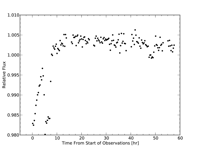
Figure 1.— width=3in

MIPS 24 µm photometry of the HD 209458 system, showing the detector ramp (0–10 h), transit (5 h), and eclipse (48 h). For plotting purposes the data have been binned to lower temporal resolution. A slight ($\sim 0.2\%$) flux decrease is apparent from 10–58 h. This could be influenced by planetary phase variations, but the similarity to the purely instrumental effects seen in Figure LABEL:fig:young_mipscal precludes an unambiguous distinction between the two effects.

To test this hypothesis, we look for evidence of persistence in our data. Using all frames taken at the second dither position we compute the median image from each of several Astronomical Observing Requests (AORs). An AOR is a Spitzer logistical unit comprising some dozens of frames; in our data set each AOR lasts approximately 3 hr. We see faint afterimages at the other thirteen dither positions when we subtract the first median AOR frame from the final median AOR frame (taken $\sim 56$ hr later; cf. Figure LABEL:fig:crossfield_raw_timeseries), which suggests that the level of persistence (a byproduct of charge trapping) increases over the course of the observations. These afterimages are much fainter when comparing data from the first and second AORs (separated by 3.6 hr), consistent with the conclusion that the level of persistence does not saturate to a constant value on these short time scales. The afterimages are not apparent by eye when comparing the last and penultimate AORs (again separated by 3.6 hr), which suggests that the charge trapping persistence has saturated by this time, as expected from the much-flattened data ramp seen in Figure LABEL:fig:crossfield_raw_timeseries.

The IRAC ramp is known to exhibit a behavior which depends on the level of illumination, with more intensely illuminated pixels exhibiting a steeper initial ramp and saturating more quickly (these pixels’ charge traps are filled more quickly because more free photoelectrons are available). We see a hint of this behavior in our data. Though pointing variations prevent us from tracking the response of individual pixels, we extract photometry (again via PSF fitting) using both 3- and 5-pixel-wide square apertures. The 3-pixel photometry – which is weighted somewhat more heavily by the most intensely illuminated pixels than is the 5-pixel photometry – shows a hint of a steeper ramp. We take this as further tentative support for our hypothesis that our ramp has a common origin with the IRAC ramp. The ramp behavior remains unchanged when we use a wider aperture, but this may not be diagnostic since the gradient in illumination level quickly flattens out beyond a few pixels.

We would like to know why we see this ramp, especially considering that no previous MIPS observations detected this effect. However, we can find no consistent discriminant between the presence or absence of a ramp in MIPS data and the state of either instrument or observatory. The first set of AORs in C10’s observations (the first $\sim 10$ hr) were anomalously low ($\sim 0.3\%$) compared to subsequent observations, which they attributed to a thermal anneal of the 24 µm detector conducted $<1$ h before these observations. No ramp was observed in the continuous, long-duration MIPS observations of either Knutson et al. (2009b) or C10, which were taken $\gtrsim 1$ day after the last 24 µm anneal. The photometry shown in Figure LABEL:fig:crossfield_raw_timeseries also occurred $>1$ day after the last 24 µm anneal, so annealing seems unlikely to explain the presence of the ramp in our data.

We investigated whether preflashing could explain the absence of any ramp in other MIPS phase curve observations. To preflash is to conduct a set of brief ($<1$ hr) observations of a bright target before observing a fainter exoplanet system (Seager & Deming, 2009; Knutson et al., 2011); experience shows that this tends to reduce the amplitude of the ramp, presumably by partially saturating the detector’s charge traps. HD 209458 is the faintest of the three exoplanet systems with long-duration MIPS 24 µm observations, but the flux difference ($\sim$20 mJy for HD 209458 vs. $\sim 60$ mJy for HD 189733) does not seem sufficiently large for only one of our five observations of HD 209458 to fail to pre-flash the detector. If the difference were due to the increased flux from HD 189733, we should still see a shorter, steeper ramp at the start of these observations. That no ramp has been reported previously, and that we see a ramp in the HD 209458 data only intermittently, suggests that some other phenomenon may be at work here.

The phase curve observations of both HD 189733 and HD 209458 began immediately after a data downlink to Earth, so this factor also does not distinguish between the cases. Prior to the data downlinks, our 2008 observations of HD 209458 were preceded by 24 µm observations of the faint RXCJ0145.2-6033 ($\sim 4$ mJy), but no 24 µm observations whatsoever were made in the $\sim$day leading up to Knutson et al. (2009b)’s observations of HD 189733. While MIPS was operational all its arrays were continuously exposed to the sky: although the Spitzer operations staff planned observations so as to avoid placing bright sources on the 24 µm array (using IRAS 25 µm images as a guide; A. Noriega-Crespo, private communication) we cannot dismiss the possibility that occasionally some bright sources may have been missed.

Thus we cannot conclusively determine why the MIPS observations of HD 209458 we present here show the detector ramp while previous, comparable observations have not shown such an effect. Nonetheless, the similarity between our photometry in Figure LABEL:fig:crossfield_raw_timeseries and raw IRAC 8 µm photometry (e.g., Agol et al., 2010) strongly suggests that the most likely explanation involves detector response variations due to charge-trapping.

3.2. The Fallback

After the detector ramp, the photometry in Figure LABEL:fig:crossfield_raw_timeseries decreases over the rest of the observations by $\sim 0.2\%$; we term this flux diminution the “fallback.” The amplitude of this effect is of the approximate amplitude expected for a 24 µm planetary thermal phase curve (Showman et al., 2009; Burrows et al., 2010), so our first inclination was to ascribe a planetary origin to this flux decrease. However, there is a distinct qualitative similarity between the phase curve photometry and pre-launch calibration data taken with the MIPS 24 µm detector under bright (170 MJy sr^-1) illumination, shown in Figure LABEL:fig:young_mipscal (reproduced from Young et al., 2003). A comparison of this figure and Figure LABEL:fig:crossfield_raw_timeseries reveals that both display the same qualitative signature of an early, steep ramp followed by a slow, gradual fallback in measured flux. The only differences are (1) an initial steep decrease in flux in the calibration data not seen in our stellar photometry (attributed by Young et al., 2003, to the response of the detector to a thermal anneal immediately preceding the data shown), and (2) longer ramp and fallback time constants in our data set.

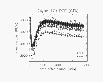
Figure 2.— width=3in

Lab calibration data for the MIPS 24 µm array, taken from Young et al. (2003; their Figure 7). The relevant data for comparison with Spitzer/MIPS observations are the gray diamonds labeled SUR (Sample Up the Ramp, the algorithm used to compute MIPS data numbers from pixel slopes). Young et al. (2003) suggest that the initial sensitivity decrease (0–50 minutes) is related to detector response variations related to a thermal anneal immediately preceding the data; as we describe in Sec. 3, our data should not be affected by any anneal operations. The rest of the observations appear strikingly similar to our photometry of HD 209458, shown in Figure LABEL:fig:crossfield_raw_timeseries. For comparison with Figure LABEL:fig:crossfield_raw_timeseries the peak pixel fluxes in the HD 209458 data frames are roughly 1000 DN/s.

The brightest pixels in the HD 209458 MIPS observations reach a flux of 45 MJy sr^-1 (corresponding to 1000 DN s^-1). Perhaps, like in some preflashed IRAC observations (cf. Knutson et al., 2011), the lower illumination level in the HD 209458 photometry (relative to the stimulation response curve from Young et al., 2003) is responsible for the different timescales evident in the two 24 µm time series. However, the brightest pixels in the observations of C10 reached a flux of 9000 DN s^-1 and no fallback is apparent in the continuous portion of those observations (though C10’s continuous photometry did decrease monotonically by $\sim 0.1\,\%$, they demonstrated a coherent planetary phase curve in two data sets spanning several years: thus planetary emission, rather than an instrumental sensitivity variation, seems a more likely interpretation of their results). Similarly, no fallback is seen in MIPS observations of HD 189733b (peak pixel flux $\sim 1200$ DN s^-1; Knutson et al., 2009b) or of the fainter eclipsing M binary GU Boo ($\lesssim 500$ DN s^-1; von Braun et al., 2008). Thus is seems possible that the fallback is linked to the presence of the detector ramp, which also appears only in our MIPS data set.

We try a number of different functional forms to fit to the $\sim 0.2\%$ post-ramp fallback, which we fit simultaneously with the ramp. These include a flat model (i.e., no decrease), sinusoidal and Lambertian profiles with arbitrary amplitude and phase (representative of a planetary phase curve), and a double-exponential of the form $(1-\alpha e^{-t/\tau_{1}})\times e^{-t/\tau_{2}}$, with $\tau_{2}\gg\tau_{1}$, motivated by the detector response variations seen in Figure LABEL:fig:young_mipscal. We decide which of these models is the most appropriate on the basis of the Bayesian Information Criterion (BIC). The model consisting of a ramp plus a decaying exponential gives the lowest BIC: $\sim 15$ units lower than obtained with the sinusoidal or Lambertian models. Thus the data prefer an instrumental explanation for the low-level flux variations that we see.

When using a sinusoidal or Lambertian model, the best-fit phase curve parameters describe a thermal phase variation which peaks well before secondary eclipse, suggesting a planetary hot spot eastward of the substellar point. Qualitatively, such a shift is consistent with observations of both HD 189733b (Knutson et al., 2009b) and $\upsilon$ And b (C10). However, the phase offset determined by this fitting process is surprisingly large: $136\deg\pm 18\deg$, a result which would seem to imply that the planet’s night side is hotter than its day side. Such a scenario has been predicted by some models (cf. Cho et al., 2003), but such a large phase offset is bigger than observed for either $\upsilon$ And b or HD 189733b, and larger still when compared to expectations for this planet from more recent simulations (e.g., Rauscher et al., 2008; Showman et al., 2009). We thus deem the phase curve fit with large offset to be an unlikely result, providing one more reason to doubt that the flux variation we see is of planetary origin.

We also inject into the data a sinusoidal phase curve with zero phase offset and a peak-to-valley amplitude equal to our best-fit secondary eclipse depth results and repeat our analysis: in this case the best-fit sinusoidal and Lambertian models have a lower BIC value (by 12 units) than the instrumental model, though the recovered amplitude and phase offset are still somewhat biased by the flux fallback. Although these results suggest that we are close to achieving the sensitivity required to constrain HD 209458b’s thermal phase variations, our ignorance of the detailed morphology of the flux fallback prevents us from reaching a more quantitative conclusion. Thus, we can only conclude that the striking qualitative similarity between Figures LABEL:fig:crossfield_raw_timeseries and LABEL:fig:young_mipscal precludes us from making any definite claims as to the detection of planetary phase curve effects in our data.

3.3. Instrument Stability

As observed previously by C10, the background flux of continuous MIPS photometry exhibits a roughly linear trend with time, with smaller, abrupt changes from one AOR to the next. The linear trend can be explained by a variation in the thermal zodiacal light as Spitzer’s perspective of HD 209458 changes with respect to the solar system, and C10 attribute the discontinuous, AOR-by-AOR background fluctuations to scattered light. Whatever the cause, these discontinuities are removed by the sky background subtraction, and do not appear to affect the final stellar photometry.

During our 2008 observations we see a 0.5 $\mu$A increase in the 24 µm detector anneal current (MIPS data file keyword AD24ANLI), a decrease of 6 mK in the scan mirror temperature (keyword ACSMMTMP), and swings in the electronics box temperature (keyword ACEBOXTM) of up to 0.3 K. During sustained observations the electronics box appears to experience heating with some time lag, but with a much shorter cooling lag during observational breaks to transmit data to Earth. Upon reexamination of past observations, we find that these three parameters exhibit similar behavior during observations of HD 189733b (Knutson et al., 2009a) and of upsilon Andromeda b (C10). The MIPS optical train is cryogenically cooled and separated from the non-cryogenic instrument electronics (Heim et al., 1998), so it does not seem likely that the observed swings in the electronics box temperature should influence the photometry. Similarly, the anneal current and scan mirror temperature do not seem to correlate with either the ramp or the post-ramp flux decrease, so we conclude that these instrumental variations do not affect our final photometry.

4. Transits

4.1. Fitting Approach

We fit transits using uniform-disk and linear limb-darkened transit models (Mandel & Agol, 2002), but (consistent with the results of Richardson et al., 2006) we find the limb-darkened model offers no improvement over the uniform-disk model (as determined by the BIC). We fit the transit data for: the time of center transit $T_{c,t}$, the impact parameter $b$, the scaled stellar radius $R_{*}/a$, the planet/star radius ratio $R_{p}/R_{*}$, and the out-of-transit system flux $F_{*}$. We hold the period fixed at $3.52474550\pm 0.00000018~{}\textrm{d}$ (Torres et al., 2008), which is a more precise determination than our observations can provide. To extract useful information from our half-transit event we always require that $b$ and $R_{*}/a$ have the same value, determined jointly from all our transits. We therefore perform one fit in which these two parameters are jointly fit, and a second fit in which we additionally fit jointly to $T_{c,t}$ and $R_{p}/R_{*}$ across all transit events.

We fit to the detector ramp in the 2008 transit by including a multiplicative factor of the form $1-\alpha e^{-t/\tau}$, where $t$ is measured from the start of the observations. This formulation of the ramp model is motivated by a physical model of the charge-trapping phenomenon thought to cause the IRAC 8 µm ramp (Agol et al., 2010). Agol et al. (2010) find a ramp based on two exponentials to be preferred for their high S/N observations, but we find that our data are not precise enough to constrain this more complicated model: when fitting a double-exponential ramp of the form $1-\alpha_{1}e^{-t/\tau_{1}}-\alpha_{2}e^{-t/\tau_{2}}$ (Agol et al., 2010) the parameters for the two exponential trends become degenerate, and the resulting fits are not preferred to the single ramp fit on the basis of the BIC. Finally, we include in all our fits the fourteen sensitivity correction terms ($c_{i}$) corresponding to the fourteen MIPS dither positions.

4.2. Results

Table 2 lists the results of the fit in which we assume a constant orbit and transit – holding $b$, $R_{*}/a$, $R_{p}/R_{*}$, and $T_{c,t}$ constant across all transits – while Table 3 lists the results of the fit in which $R_{p}/R_{*}$ and $T_{c,t}$ (but not $b$ or $R_{*}/a$) are allowed to vary between events. We plot the results of fits to each individual transit, and to the combined data set, in Figure 3. We show how the residuals to the combined fit bin down with increasing sample size in Figure LABEL:fig:bindown: the curve shown tracks closely with the $N^{-1/2}$ expectation from uncorrelated noise on short time scales ($<20$ min), but on longer time scales the residuals bin down more slowly than this. This indicates the presence of correlated (red) noise (cf. Pont et al., 2006) in these data, which is not surprising considering the ramp residuals apparent in Figure 3.

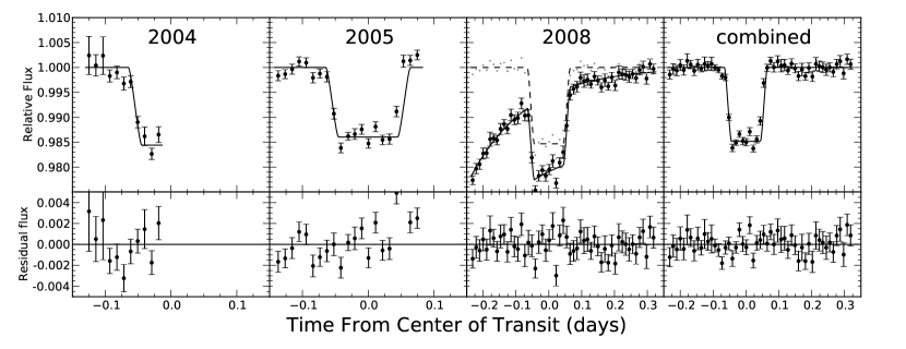
Figure 3.— MIPS 24 µm transits of HD 209458b. The top panels show photometry and the best-fit model, and the lower panels show the residuals to the fits. For plotting purposes the data have been corrected for the MIPS 14-position sensitivity variations, normalized by the stellar flux, and binned by 70 points (for the individual transits) and by 210 points (for the combined data set). We also corrected for the ramp in the 2008 data set (corrected, binned data shown as small points) before combining the data to plot the data in the rightmost panel.

Figure 4.— width=3in

Dispersion of the binned residuals (solid lines) to the combined transit and eclipse light curve fits shown in Figure 3 and 8. On longer timescales both fits exhibit a binned dispersion 10-30% higher than expected from uncorrelated noise (dashed line). The dashed lines show the expectation for uncorrelated errors, which scale as $N^{-1/2}$. The vertical dotted line indicates the transit duration.

We examine the residuals to the fourteen individual channels and see some evidence for qualitatively different correlated noise at different dither positions. We do not think it likely that this behavior is related to an intrapixel effect (as observed in IRAC; cf. Charbonneau et al., 2005), because the residual behavior we see does not correlate with mean PSF position relative to the boundaries of individual pixels. Instead, it seems more likely to be a manifestation of the known position-dependent sensitivity effect previously attributed to residual flat-fielding errors (Crossfield et al., 2010).

The resulting posterior distributions are all unimodal (except for the impact parameter $b$), and the usual correlations are apparent between $b$ and $R_{*}/a$ and between $F_{*}$ and $R_{p}/R_{*}$ (cf. Burke et al., 2007). As noted above, the 2008 transit data are strongly affected by the detector ramp, and we see correlations between the ramp parameters and the transit depth. We compute the two-dimensional posterior distributions of $R_{P}/R_{*}$, $\tau$, and $\alpha$ (marginalized over all other parameters) from the MCMC chains using the kernel density estimate approach described in C10; we show these distributions in Figure LABEL:fig:ramp_corr and list the elements of these parameters’ covariance matrix in Table 4.

Figure 5.— width=3in

Posterior distributions of the ramp parameters $(\alpha,\tau)$ and $R_{p}/R_{*}$, estimated from the MCMC analysis of the 2008 transit data. The ‘$\times$’ symbols indicate the best-fit parameters listed in Table 3, and the lines indicate the 68.27%, 95.45%, and 99.73% confidence intervals. The elements of these parameters’ covariance matrix are listed in Table 4.

4.3. Discussion

The three independently-fit transit depths listed in Table 3 have a fractional dispersion of 3%, consistent with our individual uncertainty estimates of 3-10%. We thus find no evidence for variations in transit depth, and our transit depths are consistent with the depth measured from the combination of our first two transit data sets (Richardson et al., 2006).

We plot the ensemble of HD 209458b’s transit depth measurements in Figure LABEL:fig:transmission along with a model of transit depth vs. wavelength from Fortney et al. (2010). The model is consistent with the 24 µm measurement we present here and agrees fairly well with the optical measurements of Sing et al. (2008) and the IRAC 3.6 and 4.5 µm measurements of Beaulieu et al. (2010). However, our model strongly disagrees with the IRAC 5.8 and 8.0 µm, which was also shown for the same HD 209458b model in Fortney et al. (2010). The large discrepancy remains unclear. Given the known wavelength-dependent water vapor opacity, Shabram et al. (2011) showed that reaching all four 4 IRAC data points may be impossible within the framework of a simple transmission spectrum model. Our transmission spectrum methods are described in these papers, and the atmospheric pressure-temperature profile is from a planet-wide average no-inversion model shown in Figure LABEL:fig:tpprofiles.

Figure 6.— width=3in

Measurements of the transit depth of HD 209458b: binned optical spectroscopy (Sing et al., 2008), previous mid-infrared photometry (Beaulieu et al., 2010), and our 24 µm measurement. The solid line is a model generated using the (dot-dashed) temperature-pressure profile shown in Figure LABEL:fig:tpprofiles. The solid black points without errorbars represent the weighted averages of the model over the corresponding bandpasses (indicated at bottom).

We resample the posterior distributions of the independent transit ephemerides shown in Table 3 to determine our own, independent constraint on the planet’s orbital period (assuming it is constant) using a linear relation. We compute the center-of-transit time and period to be $2453549.2075\pm 0.0013\textrm{~{}d}$ and $3.5247537\pm 0.0000049\textrm{~{}d}$, respectively; the covariance between these two parameters is $-5.652\times 10^{-9}\textrm{~{}d}^{2}$. The period we obtain differs from the established period (Torres et al., 2008) by only $8.2\times 10^{-6}\textrm{~{}d}$ (0.71 s), well within the uncertainties.

Figure 7.— width=3in

Temperature-pressure (T-P) profiles used to generate our model spectra. The dot-dashed curve is a planet-wide average T-P profile taken from a full (4$\pi$) redistribution model, and is used to model the tranmission spectrum shown in Figure LABEL:fig:transmission. It includes TiO/VO opacity, but these species have only a minor effect since nearly all of the Ti/V has condensed out of the gas phase at these cooler temperatures. The solid curve is from a model assuming no redistribution of absorbed energy (making it hotter), and includes TiO/VO to drive the temperature inversion seen in Figure LABEL:fig:emission.

5. Secondary Eclipses

5.1. Fitting Approach

We fit secondary eclipses using the uniform-disk occultation formulae of Mandel & Agol (2002), fitting each event for three astrophysical parameters: time of center of eclipse $T_{c,e}$, stellar flux $F_{*}$, and eclipse depth $F_{p}/F_{*}$ – as well as the fourteen sensitivity correction terms ($c_{i}$) discussed previously. We hold all other other orbital parameters fixed at the values listed in Torres et al. (2008), which are more precise than our constraints based on the 24 µm transit photometry. We perform four different fits: an independent fit of each eclipse taken in isolation, and a fit to the combined data set in which we fit for a single eclipse depth, but still allow $T_{c,e}$ and $F_{*}$ to vary for each event. We use only a subset of the long-duration phase curve observations to fit the 2008 eclipse, as indicated in Table 1. We tried including a linear slope in the combined eclipse fit, but this extra parameter is not justified because it gives a higher BIC than fits without such a slope.

5.2. Results

The parameters for the fit in which $T_{c,e}$ and $F_{p}/F_{*}$ are fit jointly across all eclipses (but $F_{*}$ remains independent) are shown in Table 5, and parameters for the three wholly independent eclipse fits are shown in Table 6. The data, best fit models, and residuals for all three eclipses and the combined data set are plotted in Figure 8. The only strong correlations apparent in the resulting posterior distributions are between $F_{*}$ and $F_{p}/F_{*}$ – expected since we are making a relative measurement. We show how the residuals to the combined fit bin down with increasing sample size in Figure LABEL:fig:bindown: the residuals average down more slowly than the $N^{-1/2}$ expectation from uncorrelated errors. This indicates the presence of correlated (red) noise (cf. Pont et al., 2006) in these data, which is expected given the behavior of the eclipse residuals shown in Figure 8.

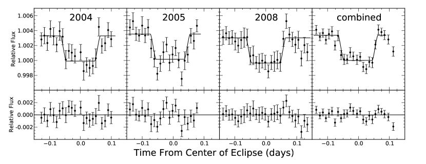
Figure 8.— MIPS 24 µm eclipses of HD 209458b. The top panels show photometry and the best-fit models, and the lower panels show the residuals to the fits. For plotting purposes the data have been corrected for the MIPS 14-position sensitivity variations, normalized by the stellar flux, and binned by 70 points (for the individual eclipses) and by 210 points (for the combined data set).

5.3. Discussion

The three eclipse depths have a dispersion of 13%, consistent with our estimated measurement errors (12-18%). We thus find no evidence for variability of planetary emission, in good agreement with general circulation models which predict HD 209458b’s MIR dayside emission will vary by $<5\%$ (e.g., Rauscher et al., 2008; Showman et al., 2009; Dobbs-Dixon et al., 2010) and consistent with the measurement that HD 189733b’s 8 µm dayside emission varies by $<2.7\,\%$(Agol et al., 2010). Our mean eclipse depth over all three epochs – $0.338\%\pm 0.026\%$ – is $\sim 1.3\sigma$ deeper than the initial measurement by Deming et al. (2005) of $0.26\%\pm 0.046\%$. We convert this eclipse depth to a brightness temperature of $1320\textrm{~{}K}\pm 80\textrm{~{}K}$ using the method outlined by C10.

We plot the ensemble of HD 209458b’s secondary eclipse measurements in Figure LABEL:fig:emission along with a model of planet/star contrast ratio vs. wavelength. The modeling procedure is described in detail in Fortney et al. (2006) and Fortney et al. (2008). Using a stellar model for the incident flux and a solar metallicity atmosphere, we derive a radiative-convective pressure-temperature profile assuming chemical equilibrium mixing ratios. The model assumes no loss of absorbed energy to the night side, and redistribution of energy over the day side only (see Fortney et al., 2008). We show the pressure-temperature profile, which feature a temperature inversion due to the absorption of stellar flux by TiO and VO gasses, in Figure LABEL:fig:tpprofiles. Clearly a stronger temperature inversion is needed, as the contrast between the IRAC 3.6 and 4.5  µm bands is not large enough. Since the 24 µm photosphere is predicted to lie at $1-10$ mbar on HD 209458b (Showman et al., 2009) our measurement indicates a somewhat cooler temperature than is expected for this planet given its atmospheric temperature inversion. The anomalously low 24 µm flux has been noted previously (e.g., Madhusudhan & Seager, 2010); taken in concert with $\upsilon$ And b’s large and still-unexplained 24 µm phase offset (C10) these results suggest that our current understanding of atmospheric opacity sources in this wavelength range may be incomplete. Alternatively, we can fit reasonably fit the 3.6, 8.0, and 24  µm points with the dayside emission of the 3D general circulation model of Showman et al. (2009), which is cooler than the corresponding 1D model from Fortney et al. (2008). Clearly more work is needed to robustly fit the dayside photometry of the planet within the framework of a 1D or 3D self-consistent model.

Figure 9.— width=3in

Measurements of the secondary eclipse depth of HD 209458b: previous Spitzer/IRAC photometry (Knutson et al., 2008) and our 24 µm measurement. The solid line is from a model assuming zero redistribution of incident flux and including gaseous TiO and VO to drive a temperature inversion; we show this model’s temperature-pressure profile in Figure LABEL:fig:tpprofiles. The dashed line is the emission spectrum from Showman et al. (2009). The solid black points without errorbars represent the weighted averages of the models over the corresponding bandpasses (indicated at bottom).

We also fit a linear relation to the three eclipse times in the same manner as in Sec. 4. We compute a period of $3.5247445\pm 0.0000097\textrm{~{}d}$, which differs from the established period (Torres et al., 2008) by $0.99\times 10^{-6}\textrm{~{}d}$ ($0.086\textrm{~{}s}$), well within the uncertainties. This value also agrees with our measurement of the period from the transit fits; the two periods differ by only $0.79\pm 0.94\textrm{~{}s}$, which is (as expected) consistent with zero.

6. Joint Orbital Constraints and System Flux

6.1. Timing and Eccentricity: Still a Chance for Winds

Measuring the times of transit and secondary eclipse constrains the quantity $e\cos\omega$, where $e$ is the planet’s orbital eccentricity and $\omega$ its longitude of periastron (Seager, 2011, chapter by J. Winn). We resample the posterior distributions of $T_{c,t}$ and $T_{c,e}$ from the fits shown in Tables 2 and 5 and compute the difference between our transit and eclipse ephemerides (i.e., $\left[T_{c,e}-T_{c,t}\right]\textrm{~{}mod~{}}P-\frac{P}{2}$) to be $32\pm 129\textrm{~{}s}$ after also accounting for the 47 s light travel time from the planet’s location during eclipse to its location during transit (Torres et al., 2008). This results constrains $e\cos\omega$ to be $0.00004\pm 0.00033$, consistent with zero and with previous constraints from radial velocity (Torres et al., 2008). We do not see the marginal timing offset previously reported (Knutson et al., 2008), which may have been biased by the higher level of correlated noise (due to the IRAC intrapixel effect) in the 3.6 and 4.5 µm IRAC data.

A measurement of $e\cos\omega$ directly constrains the apparent velocity offset that can be induced in planetary absorption lines during transit (cf. Montalto et al., 2011); this provides an independent check as to whether the recent measurement of a velocity offset of $2\pm 1\textrm{~{}km~{}s}^{-1}$ in HD 209458b (Snellen et al., 2010) can be attributed to a low, but nonzero, orbital eccentricity. Our timing measurements of HD 209458b set a $3\sigma$ upper limit on any velocity offset due to the planet’s orbital eccentricity of only $140\textrm{~{}m~{}s}^{-1}/\sqrt{1-e^{2}}$. Thus the claimed velocity offset, though still of low significance, cannot be dismissed as resulting from the HD 209458b’s orbital eccentricity.

6.2. System Flux: No Excess Detected

Although our primary science results – the transit and eclipse depths – rely on relative flux measurements, our observations also allow us to measure absolute 24 µm photometry for the HD 209458 system. Our flux measurements for this system vary from epoch to epoch by much more than our quoted statistical uncertainties, but the variations are not large compared to the $\lesssim 1\%$ repeatability and 2% absolute calibration accuracy of the MIPS 24 µm array (Engelbracht et al., 2007). Our 21 pixel aperture encloses 99.2% of the starlight (as determined from our synthetic PSF), and we account for this small effect in the value quoted below.

We therefore report the 24 µm system flux as $18.7\pm 0.4$ mJy, consistent with the flux expected from the HD 209458 stellar photosphere (as reported by Deming et al., 2005). HD 209458 was not detected by IRAS (Beichman et al., 1988), but is present in the Widefield Infrared Survey Explorer’s all-sky point source catalogue (Wright et al., 2010). The WISE photometry gives a W4 system flux of $25.74\pm 0.12$ mJy, which is higher than but marginally ($\sim 3\sigma$) consistent with the Spitzer-derived value after accounting for the different wavelengths of the two instruments. We therefore conclude that HD 209458 does not have a strong 24 µm infrared excess, as is typical of middle-aged F dwarfs (Moór et al., 2011).

7. Conclusions and Future Work

We have described a homogeneous analysis of all Spitzer MIPS observations of the hot Jupiter HD 209458b. The data comprise three eclipses, two and a half transits, and a long, continuous observation designed to observe the planet’s thermal phase curve; of these, analysis of two of the eclipses, one transit, and the phase curve observations have remained unpublished until now. The long-duration phase curve observation exhibits a detector ramp that appears similar to the ramp seen in Spitzer/IRAC 8 µm photometry, and we model this effect using the exponential function proposed by Agol et al. (2010). We also see a $\sim-0.2\%$ flux decrease in the latter portion of the phase curve observations. This fallback is similar to a known (but poorly characterized) variation in the response of the MIPS detector when subjected to bright illumination (cf. Figure LABEL:fig:young_mipscal and Young et al., 2003).

We are unable to determine why either the fallback or the ramp have not been seen in any prior MIPS observations. Despite this failure the correspondence between our photometry and the pre-launch array calibration data leads us to conclude that ramp and fallback are correlated and both are most likely of instrumental, rather than astrophysical, origin. This conclusion is strengthened by the result that fitting periodic phase functions to the data yields a planetary model hotter on its night side than its day side, strikingly at odds with theory (Rauscher et al., 2008; Showman et al., 2009; Dobbs-Dixon et al., 2010; Cowan & Agol, 2011a) and inconsistent with other published observations of hot Jupiters (Harrington et al., 2006; Knutson et al., 2007, 2009b; Crossfield et al., 2010).

We see no evidence for variation in the three eclipse depths, and a joint fit of all three eclipses gives our best estimate of the 24 µm planet/star contrast: $0.338\%\pm 0.026\%$. This value is more precise and higher than the previously published measurement (Deming et al., 2005), and corresponds to an average dayside brightness temperature of $1320\textrm{~{}K}\pm 80\textrm{~{}K}$, consistent with models of this planet’s thermal atmospheric structure (Showman et al., 2009; Madhusudhan & Seager, 2010; Moses et al., 2011). We note parenthetically that this new eclipse depth has already diffused into several papers (cf. Showman et al., 2009; Burrows et al., 2010; Madhusudhan & Seager, 2009, 2010; Fortney et al., 2010; Moses et al., 2011); the value and uncertainty quoted in those works are close to those we report here, so their conclusions should be relatively unaffected.

We see no evidence for variations in our transit measurements, and a joint fit of our two and a half transits yields a 24 µm transit depth of $1.484\%\pm 0.033\%$. The transit depth is less well-constrained than the eclipse depth because only half of the first transit was observed, and the last transit occurred during the detector ramp.

The ephemerides calculated from our analyses of the transits and eclipses allow us to compute orbital periods of $3.5247537\pm 0.0000049\textrm{~{}d}$ and $3.5247445\pm 0.0000097\textrm{~{}d}$, respectively, which are consistent with but less precise than the orbital period of Torres et al. (2008). Eclipses occur $32\pm 129\textrm{~{}s}$ earlier than would be expected from a circular orbit, which constrains the orbital quantity $e\cos\omega$ to be $0.00004\pm 0.00033$. This suggests that HD 209458b’s inflated radius (larger than predicted by models of planetary interiors; Fortney et al., 2007) cannot be explained by interior heating from ongoing tidal circularization, and that the possible velocity offset reported by Snellen et al. (2010) cannot be explained by a nonzero orbital eccentricity.

Although we obtain improved estimates of the 24 µm transit and secondary eclipse parameters, instrumental effects prevent a conclusive detection of the planet’s thermal phase curve. The phase curve signal is inextricably combined with the systematic fallback effect, despite estimates that the planet’s day/night contrast should be as large as a few parts per thousand (Showman et al., 2009). Such a large and intermittent systematic effect has profound implications for future mid-infrared exoplanet observations with EChO, SPICA, and JWST. Models of terrestrial planet phase curves predict phase amplitudes of $\lesssim 10^{-4}$ (Selsis et al., 2011; Maurin et al., 2011); such observations could be utterly confounded by the instrumental systematics seen in our observations, and so may be much more challenging that has been heretofore assumed (Kaltenegger & Traub, 2009; Seager & Deming, 2009). Although it may be possible to reduce the effect of the ramp with a pre-flash strategy similar to that adopted for the 8 µm IRAC array, a further defense against these challenges would seem to be a more comprehensive campaign of array characterization. Specifically, a detailed characterization of the detector response to sustained levels of the high illumination expected from observations of terrestrial planets around the brightest nearby stars is highly desirable, and should be considered an essential requirement for all future infrared space telescopes.

Table 1Spitzer/MIPS 24 µm Observations of HD 209458b

UT Date	Event	Duration (hr)	tint (s)	Nexposures	Bkd (MJy Sr-1)	$\Delta t$ (s)
UT 2004 Dec 5	Half transit	2.8	8.91	840	28.8	-544
UT 2004 Dec 6	Eclipse	5.8	9.96	1680	29.2	-531
UT 2005 Jun 27	Transit	5.6	9.96	1680	28.9	-612
UT 2005 Dec 1	Eclipse	5.6	9.96	1680	26.7	+183
UT 2008 Jul 25	Transit	14.2	9.96	4060	28.3	-649
UT 2008 Jul 27	Eclipse	6.9	9.96	2072	27.9	-663

Table 2 Joint Transit Fits

Parameter	2004	2005	2008
$c_{0}$	+0.0009 $\pm$ 0.0022	+0.00036 $\pm$ 0.00086	+0.00274 $\pm$ 0.00053
$c_{1}$	+0.0097 $\pm$ 0.0027	+0.00881 $\pm$ 0.00088	+0.01387 $\pm$ 0.00055
$c_{2}$	-0.0030 $\pm$ 0.0022	+0.00101 $\pm$ 0.00136	+0.00487 $\pm$ 0.00053
$c_{3}$	+0.0106 $\pm$ 0.0024	+0.00866 $\pm$ 0.00079	+0.00858 $\pm$ 0.00056
$c_{4}$	-0.0034 $\pm$ 0.0024	+0.00148 $\pm$ 0.00115	-0.00020 $\pm$ 0.00053
$c_{5}$	-0.0021 $\pm$ 0.0032	+0.01006 $\pm$ 0.00080	+0.01310 $\pm$ 0.00052
$c_{6}$	+0.0017 $\pm$ 0.0022	-0.00574 $\pm$ 0.00078	-0.00502 $\pm$ 0.00057
$c_{7}$	-0.0023 $\pm$ 0.0033	+0.00167 $\pm$ 0.00081	-0.00720 $\pm$ 0.00054
$c_{8}$	-0.0036 $\pm$ 0.0023	-0.00298 $\pm$ 0.00078	-0.00121 $\pm$ 0.00058
$c_{9}$	+0.0098 $\pm$ 0.0023	-0.00324 $\pm$ 0.00135	-0.00919 $\pm$ 0.00060
$c_{10}$	-0.0032 $\pm$ 0.0028	+0.00394 $\pm$ 0.00111	+0.00210 $\pm$ 0.00057
$c_{11}$	-0.0126 $\pm$ 0.0032	-0.00974 $\pm$ 0.00103	-0.01016 $\pm$ 0.00057
$c_{12}$	+0.0008 $\pm$ 0.0028	-0.00039 $\pm$ 0.00085	-0.00122 $\pm$ 0.00065
$c_{13}$	-0.0028 $\pm$ 0.0024	-0.01360 $\pm$ 0.00091	-0.01062 $\pm$ 0.00052
$F_{*}$ [mJy]	+18.845 $\pm$ 0.012	+18.7784 $\pm$ 0.0049	+18.696 $\pm$ 0.010
$\alpha$	–	–	+0.02437 $\pm$ 0.00068
$\tau$ [d]	–	–	+0.174 $\pm$ 0.016
$T_{c,t}$ [BJDTDB]		2453549.20852 $\pm$ 0.00049
$b$		+0.590 $\pm$ 0.062
$R_{*}/a$		+0.1205 $\pm$ 0.0066
$R_{p}/R_{*}$		+0.1218 $\pm$ 0.0014
$(R_{p}/R_{*})^{2}$		+0.01483 $\pm$ 0.00033

Table 3 Semi-Joint Transit Fits

Parameter	2004	2005	2008
$c_{0}$	-0.0001 $\pm$ 0.0024	+0.00043 $\pm$ 0.00084	+0.00268 $\pm$ 0.00054
$c_{1}$	+0.0091 $\pm$ 0.0030	+0.00866 $\pm$ 0.00095	+0.01368 $\pm$ 0.00053
$c_{2}$	-0.0032 $\pm$ 0.0022	+0.00087 $\pm$ 0.00149	+0.00524 $\pm$ 0.00076
$c_{3}$	+0.0117 $\pm$ 0.0023	+0.00872 $\pm$ 0.00082	+0.00878 $\pm$ 0.00066
$c_{4}$	-0.0032 $\pm$ 0.0023	+0.00146 $\pm$ 0.00110	-0.00016 $\pm$ 0.00053
$c_{5}$	-0.0021 $\pm$ 0.0029	+0.01009 $\pm$ 0.00078	+0.01316 $\pm$ 0.00053
$c_{6}$	+0.0019 $\pm$ 0.0022	-0.00603 $\pm$ 0.00084	-0.00516 $\pm$ 0.00053
$c_{7}$	-0.0019 $\pm$ 0.0039	+0.00157 $\pm$ 0.00083	-0.00686 $\pm$ 0.00058
$c_{8}$	-0.0039 $\pm$ 0.0023	-0.00301 $\pm$ 0.00078	-0.00110 $\pm$ 0.00063
$c_{9}$	+0.0095 $\pm$ 0.0022	-0.00317 $\pm$ 0.00144	-0.00910 $\pm$ 0.00057
$c_{10}$	-0.0032 $\pm$ 0.0029	+0.00378 $\pm$ 0.00093	+0.00189 $\pm$ 0.00052
$c_{11}$	-0.0124 $\pm$ 0.0028	-0.00942 $\pm$ 0.00082	-0.00977 $\pm$ 0.00056
$c_{12}$	+0.0007 $\pm$ 0.0028	-0.00035 $\pm$ 0.00086	-0.00189 $\pm$ 0.00129
$c_{13}$	-0.0026 $\pm$ 0.0022	-0.01330 $\pm$ 0.00078	-0.01096 $\pm$ 0.00061
$T_{c,t}$ [BJDTDB]	2453344.7718 $\pm$ 0.0025	2453549.20746 $\pm$ 0.00065	2454673.60391 $\pm$ 0.00074
$R_{p}/R_{*}$	+0.1227 $\pm$ 0.0060	+0.1189 $\pm$ 0.0020	+0.1238 $\pm$ 0.0019
$F_{*}$ [mJy]	+18.850 $\pm$ 0.016	+18.7735 $\pm$ 0.0056	+18.6947 $\pm$ 0.0095
$(R_{p}/R_{*})^{2}$	+0.0151 $\pm$ 0.0015	+0.01413 $\pm$ 0.00046	+0.01531 $\pm$ 0.00046
$\alpha$	–	–	+0.02458 $\pm$ 0.00071
$\tau$ [d]	–	–	+0.168 $\pm$ 0.016
$b$		+0.581 $\pm$ 0.070
$R_{*}/a$		+0.1197 $\pm$ 0.0069

Table 4Ramp and transit depth covariance matrix (cf. Figure LABEL:fig:ramp_corr).

Element	$\textrm{Value}/10^{6}$
$\sigma^{2}_{\alpha}$	0.507
$\sigma^{2}_{\tau[d]}$	266 d2
$\sigma^{2}_{R_{p}/R_{*}}$	3.49
$\sigma_{\alpha,\tau[d]}$	-5.03 d
$\sigma_{\alpha,R_{p}/R_{*}}$	0.379
$\sigma_{\tau[d],R_{p}/R_{*}}$	-16.3 d

Table 5Joint Eclipse Fits

Parameter	2004	2005	2008
$c_{0}$	+0.00298 $\pm$ 0.00080	+0.00048 $\pm$ 0.00078	+0.00278 $\pm$ 0.00073
$c_{1}$	+0.00793 $\pm$ 0.00078	+0.01103 $\pm$ 0.00080	+0.01331 $\pm$ 0.00071
$c_{2}$	+0.00619 $\pm$ 0.00079	+0.00349 $\pm$ 0.00078	+0.00397 $\pm$ 0.00074
$c_{3}$	+0.00943 $\pm$ 0.00075	+0.00879 $\pm$ 0.00078	+0.00887 $\pm$ 0.00071
$c_{4}$	+0.00048 $\pm$ 0.00108	+0.00186 $\pm$ 0.00102	-0.00002 $\pm$ 0.00074
$c_{5}$	+0.01148 $\pm$ 0.00080	+0.01151 $\pm$ 0.00079	+0.01480 $\pm$ 0.00069
$c_{6}$	-0.00557 $\pm$ 0.00079	-0.00461 $\pm$ 0.00084	-0.00432 $\pm$ 0.00072
$c_{7}$	-0.00571 $\pm$ 0.00082	-0.00582 $\pm$ 0.00079	-0.00514 $\pm$ 0.00072
$c_{8}$	-0.00171 $\pm$ 0.00078	-0.00020 $\pm$ 0.00082	-0.00329 $\pm$ 0.00070
$c_{9}$	-0.00231 $\pm$ 0.00079	-0.00361 $\pm$ 0.00079	-0.00754 $\pm$ 0.00070
$c_{10}$	+0.00052 $\pm$ 0.00082	+0.00084 $\pm$ 0.00093	-0.00137 $\pm$ 0.00080
$c_{11}$	-0.00691 $\pm$ 0.00081	-0.00973 $\pm$ 0.00076	-0.00712 $\pm$ 0.00073
$c_{12}$	-0.00507 $\pm$ 0.00082	-0.00402 $\pm$ 0.00078	-0.00333 $\pm$ 0.00072
$c_{13}$	-0.01142 $\pm$ 0.00079	-0.00968 $\pm$ 0.00081	-0.01121 $\pm$ 0.00071
$F_{*}$ [mJy]	+18.78683 $\pm$ 0.00486	+18.70529 $\pm$ 0.00485	+18.60906 $\pm$ 0.00472
$F_{p}/F_{*}$		+0.00338 $\pm$ 0.00026
$T_{B}$ [K]		+1310 $\pm$ 80
$F_{p}$ [$\mu$Jy]		+63.2 $\pm$ 4.9
$T_{c,e}$ [BJD TDB]		2453706.0595 $\pm$ 0.0014

Table 6Independent Eclipse Fits

Parameter	2004	2005	2008
$c_{0}$	0.00262 $\pm$ 0.00090	-0.00020 $\pm$ 0.00112	0.00044 $\pm$ 0.00264
$c_{1}$	0.00744 $\pm$ 0.00089	0.01028 $\pm$ 0.00124	0.01246 $\pm$ 0.00114
$c_{2}$	0.00500 $\pm$ 0.00169	0.00396 $\pm$ 0.00084	0.00449 $\pm$ 0.00106
$c_{3}$	0.00879 $\pm$ 0.00101	0.00879 $\pm$ 0.00077	0.00850 $\pm$ 0.00075
$c_{4}$	-0.00042 $\pm$ 0.00090	0.00198 $\pm$ 0.00111	0.00143 $\pm$ 0.00160
$c_{5}$	0.01090 $\pm$ 0.00104	0.01109 $\pm$ 0.00091	0.01392 $\pm$ 0.00115
$c_{6}$	-0.00488 $\pm$ 0.00106	-0.00502 $\pm$ 0.00109	-0.00351 $\pm$ 0.00120
$c_{7}$	-0.00453 $\pm$ 0.00138	-0.00331 $\pm$ 0.00284	-0.00561 $\pm$ 0.00086
$c_{8}$	-0.00248 $\pm$ 0.00109	-0.00078 $\pm$ 0.00089	-0.00249 $\pm$ 0.00105
$c_{9}$	-0.00230 $\pm$ 0.00082	-0.00239 $\pm$ 0.00142	-0.00744 $\pm$ 0.00073
$c_{10}$	0.00113 $\pm$ 0.00118	0.00086 $\pm$ 0.00093	0.00079 $\pm$ 0.00225
$c_{11}$	-0.00588 $\pm$ 0.00118	-0.01021 $\pm$ 0.00097	-0.01012 $\pm$ 0.00328
$c_{12}$	-0.00315 $\pm$ 0.00201	-0.00385 $\pm$ 0.00078	-0.00189 $\pm$ 0.00171
$c_{13}$	-0.01197 $\pm$ 0.00104	-0.01090 $\pm$ 0.00166	-0.01059 $\pm$ 0.00098
$T_{c,e}$ [BJD TDB]	2453346.5348 $\pm$ 0.0028	2453706.0600 $\pm$ 0.0029	2454675.3639 $\pm$ 0.0026
$F_{p}/F_{*}$	0.00325 $\pm$ 0.00053	0.00384 $\pm$ 0.00046	0.00281 $\pm$ 0.00051
$T_{B}$ [K]	1270 $\pm$ 190	1450$\pm$ 230	1130 $\pm$ 160
$F_{*}$ [mJy]	18.7884 $\pm$ 0.0069	18.7023 $\pm$ 0.0064	18.6155 $\pm$ 0.0068
$F_{p}$ [$\mu$Jy]	61.1 $\pm$ 10.0	71.9 $\pm$ 8.6	52.3 $\pm$ 9.5

References

- Agol et al. (2010) Agol, E., Cowan, N. B., Knutson, H. A., Deming, D., Steffen, J. H., Henry, G. W., & Charbonneau, D. 2010, ApJ, 721, 1861, ADS, 1007.4378
- Baines et al. (2008) Baines, E. K., McAlister, H. A., ten Brummelaar, T. A., Turner, N. H., Sturmann, J., Sturmann, L., Goldfinger, P. J., & Ridgway, S. T. 2008, ApJ, 680, 728, ADS, 0803.1411
- Beaulieu et al. (2010) Beaulieu, J. P. et al. 2010, MNRAS, 409, 963, ADS, 0909.0185
- Beichman et al. (1988) Beichman, C. A., Neugebauer, G., Habing, H. J., Clegg, P. E., & Chester, T. J., eds. 1988, Infrared astronomical satellite (IRAS) catalogs and atlases. Volume 1: Explanatory supplement, Vol. 1, ADS
- Bouchy et al. (2005) Bouchy, F. et al. 2005, A&A, 444, L15, ADS, arXiv:astro-ph/0510119
- Brown et al. (2001) Brown, T. M., Charbonneau, D., Gilliland, R. L., Noyes, R. W., & Burrows, A. 2001, ApJ, 552, 699, ADS, arXiv:astro-ph/0101336
- Burke et al. (2007) Burke, C. J. et al. 2007, ApJ, 671, 2115, ADS, 0705.0003
- Burrows et al. (2008) Burrows, A., Budaj, J., & Hubeny, I. 2008, ApJ, 678, 1436, ADS, 0709.4080
- Burrows et al. (2007) Burrows, A., Hubeny, I., Budaj, J., & Hubbard, W. B. 2007, ApJ, 661, 502, arXiv:astro-ph/0612703
- Burrows et al. (2010) Burrows, A., Rauscher, E., Spiegel, D. S., & Menou, K. 2010, ApJ, 719, 341, ADS, 1005.0346
- Charbonneau et al. (2005) Charbonneau, D. et al. 2005, ApJ, 626, 523, ADS, arXiv:astro-ph/0503457
- Charbonneau et al. (2000) Charbonneau, D., Brown, T. M., Latham, D. W., & Mayor, M. 2000, ApJ, 529, L45, ADS, arXiv:astro-ph/9911436
- Charbonneau et al. (2002) Charbonneau, D., Brown, T. M., Noyes, R. W., & Gilliland, R. L. 2002, ApJ, 568, 377, ADS, arXiv:astro-ph/0111544
- Charbonneau et al. (2008) Charbonneau, D., Knutson, H. A., Barman, T., Allen, L. E., Mayor, M., Megeath, S. T., Queloz, D., & Udry, S. 2008, ApJ, 686, 1341, ADS, 0802.0845
- Cho et al. (2008) Cho, J., Menou, K., Hansen, B. M. S., & Seager, S. 2008, ApJ, 675, 817, ADS
- Cho et al. (2003) Cho, J. Y.-K., Menou, K., Hansen, B. M. S., & Seager, S. 2003, ApJ, 587, L117, ADS, arXiv:astro-ph/0209227
- Colbert, J. (2011) Colbert, J., ed. 2011, MIPS Instrument Handbook, v3.0
- Cooper & Showman (2005) Cooper, C. S., & Showman, A. P. 2005, ApJ, 629, L45, ADS, arXiv:astro-ph/0502476
- Cowan & Agol (2011a) Cowan, N. B., & Agol, E. 2011a, ApJ, 726, 82, ADS, 1011.0428
- Cowan & Agol (2011b) —. 2011b, ApJ, 729, 54, ADS, 1001.0012
- Cowan et al. (2007) Cowan, N. B., Agol, E., & Charbonneau, D. 2007, MNRAS, 379, 641, ADS, 0705.1189
- Crossfield et al. (2010) Crossfield, I. J. M., Hansen, B. M. S., Harrington, J., Cho, J. Y.-K., Deming, D., Menou, K., & Seager, S. 2010, ApJ, 723, 1436, ADS, 1008.0393
- Deming et al. (2006) Deming, D., Harrington, J., Seager, S., & Richardson, L. J. 2006, ApJ, 644, 560, ADS, arXiv:astro-ph/0602443
- Deming et al. (2005) Deming, D., Seager, S., Richardson, L. J., & Harrington, J. 2005, Nature, 434, 740, ADS, arXiv:astro-ph/0503554
- Désert et al. (2008) Désert, J.-M., Vidal-Madjar, A., Lecavelier Des Etangs, A., Sing, D., Ehrenreich, D., Hébrard, G., & Ferlet, R. 2008, A&A, 492, 585, ADS, 0809.1865
- Dobbs-Dixon et al. (2010) Dobbs-Dixon, I., Cumming, A., & Lin, D. N. C. 2010, ApJ, 710, 1395, ADS, 1001.0982
- Eastman et al. (2010) Eastman, J., Siverd, R., & Gaudi, B. S. 2010, PASP, 122, 935, ADS, 1005.4415
- Engelbracht et al. (2007) Engelbracht, C. W. et al. 2007, PASP, 119, 994, ADS, 0704.2195
- Fortney et al. (2006) Fortney, J. J., Cooper, C. S., Showman, A. P., Marley, M. S., & Freedman, R. S. 2006, ApJ, 652, 746, ADS, arXiv:astro-ph/0608235
- Fortney et al. (2008) Fortney, J. J., Lodders, K., Marley, M. S., & Freedman, R. S. 2008, ApJ, 678, 1419, ADS, 0710.2558
- Fortney et al. (2007) Fortney, J. J., Marley, M. S., & Barnes, J. W. 2007, ApJ, 659, 1661, arXiv:astro-ph/0612671
- Fortney et al. (2010) Fortney, J. J., Shabram, M., Showman, A. P., Lian, Y., Freedman, R. S., Marley, M. S., & Lewis, N. K. 2010, ApJ, 709, 1396, ADS, 0912.2350
- Harrington et al. (2006) Harrington, J., Hansen, B. M., Luszcz, S. H., Seager, S., Deming, D., Menou, K., Cho, J., & Richardson, L. J. 2006, Science, 314, 623, ADS
- Heim et al. (1998) Heim, G. B. et al. 1998, 3356, 985, ADS
- Heng et al. (2011a) Heng, K., Frierson, D. M. W., & Phillipps, P. J. 2011a, MNRAS, 418, 2669, ADS, 1105.4065
- Heng et al. (2011b) Heng, K., Menou, K., & Phillipps, P. J. 2011b, MNRAS, 413, 2380, ADS, 1010.1257
- Henry et al. (2000) Henry, G. W., Marcy, G. W., Butler, R. P., & Vogt, S. S. 2000, ApJ, 529, L41, ADS
- Kaltenegger & Traub (2009) Kaltenegger, L., & Traub, W. A. 2009, ApJ, 698, 519, ADS, 0903.3371
- Knutson et al. (2008) Knutson, H. A., Charbonneau, D., Allen, L. E., Burrows, A., & Megeath, S. T. 2008, ApJ, 673, 526, ADS, 0709.3984
- Knutson et al. (2007) Knutson, H. A. et al. 2007, Nature, 447, 183, ADS, 0705.0993
- Knutson et al. (2009a) Knutson, H. A., Charbonneau, D., Cowan, N. B., Fortney, J. J., Showman, A. P., Agol, E., & Henry, G. W. 2009a, ApJ, 703, 769, ADS, 0908.1977
- Knutson et al. (2009b) Knutson, H. A. et al. 2009b, ApJ, 690, 822, ADS, 0802.1705
- Knutson et al. (2010) Knutson, H. A., Howard, A. W., & Isaacson, H. 2010, ApJ, 720, 1569, ADS, 1004.2702
- Knutson et al. (2011) Knutson, H. A. et al. 2011, ApJ, 735, 27, ADS, 1104.2901
- Madhusudhan et al. (2011a) Madhusudhan, N. et al. 2011a, Nature, 469, 64, ADS, 1012.1603
- Madhusudhan et al. (2011b) Madhusudhan, N., Mousis, O., Johnson, T. V., & Lunine, J. I. 2011b, ArXiv e-prints, ADS, 1109.3183
- Madhusudhan & Seager (2009) Madhusudhan, N., & Seager, S. 2009, ApJ, 707, 24, ADS, 0910.1347
- Madhusudhan & Seager (2010) —. 2010, ApJ, 725, 261, ADS, 1010.4585
- Mandel & Agol (2002) Mandel, K., & Agol, E. 2002, ApJ, 580, L171, ADS
- Maurin et al. (2011) Maurin, A. S., Selsis, F., Hersant, F., & Belu, A. 2011, ArXiv e-prints, ADS, 1110.3087
- Mayor & Queloz (1995) Mayor, M., & Queloz, D. 1995, Nature, 378, 355, ADS
- Mazeh et al. (2000) Mazeh, T. et al. 2000, ApJ, 532, L55, ADS, arXiv:astro-ph/0001284
- Montalto et al. (2011) Montalto, M., Santos, N. C., Boisse, I., Boué, G., Figueira, P., & Sousa, S. 2011, A&A, 528, L17, ADS, 1102.0464
- Moór et al. (2011) Moór, A. et al. 2011, ApJS, 193, 4, ADS, 1012.3631
- Moses et al. (2011) Moses, J. I. et al. 2011, ApJ, 737, 15, ADS, 1102.0063
- Pont et al. (2006) Pont, F., Zucker, S., & Queloz, D. 2006, MNRAS, 373, 231, ADS, arXiv:astro-ph/0608597
- Rauscher & Menou (2010) Rauscher, E., & Menou, K. 2010, ApJ, 714, 1334, ADS, 0907.2692
- Rauscher & Menou (2012) —. 2012, ApJ, 745, 78, ADS, 1105.2321
- Rauscher et al. (2008) Rauscher, E., Menou, K., Cho, J., Seager, S., & Hansen, B. M. S. 2008, ApJ, 681, 1646, ADS, 0712.2242
- Richardson et al. (2003) Richardson, L. J., Deming, D., & Seager, S. 2003, ApJ, 597, 581, arXiv:astro-ph/0307297
- Richardson et al. (2006) Richardson, L. J., Harrington, J., Seager, S., & Deming, D. 2006, ApJ, 649, 1043, ADS, arXiv:astro-ph/0606096
- Rieke et al. (2004) Rieke, G. H. et al. 2004, in Presented at the Society of Photo-Optical Instrumentation Engineers (SPIE) Conference, Vol. 5487, Society of Photo-Optical Instrumentation Engineers (SPIE) Conference Series, ed. J. C. Mather, 50–61, ADS
- Rowe et al. (2008) Rowe, J. F. et al. 2008, ApJ, 689, 1345, ADS, 0711.4111
- Schuler et al. (2011) Schuler, S. C., Flateau, D., Cunha, K., King, J. R., Ghezzi, L., & Smith, V. V. 2011, ApJ, 732, 55, ADS, 1103.0757
- Seager (2011) Seager, S. 2011, Exoplanets, ed. Piper, S., ADS
- Seager & Deming (2009) Seager, S., & Deming, D. 2009, ApJ, 703, 1884, ADS, 0910.1505
- Seager & Sasselov (2000) Seager, S., & Sasselov, D. D. 2000, ApJ, 537, 916, ADS, arXiv:astro-ph/9912241
- Selsis et al. (2011) Selsis, F., Wordsworth, R. D., & Forget, F. 2011, A&A, 532, A1+, ADS, 1104.4763
- Shabram et al. (2011) Shabram, M., Fortney, J. J., Greene, T. P., & Freedman, R. S. 2011, ApJ, 727, 65, ADS, 1010.2451
- Showman et al. (2009) Showman, A. P., Fortney, J. J., Lian, Y., Marley, M. S., Freedman, R. S., Knutson, H. A., & Charbonneau, D. 2009, ApJ, 699, 564, ADS
- Showman & Guillot (2002) Showman, A. P., & Guillot, T. 2002, A&A, 385, 166, ADS, arXiv:astro-ph/0202236
- Sing et al. (2009) Sing, D. K., Désert, J., Lecavelier Des Etangs, A., Ballester, G. E., Vidal-Madjar, A., Parmentier, V., Hebrard, G., & Henry, G. W. 2009, A&A, 505, 891, ADS, 0907.4991
- Sing et al. (2008) Sing, D. K., Vidal-Madjar, A., Lecavelier des Etangs, A., Désert, J., Ballester, G., & Ehrenreich, D. 2008, ApJ, 686, 667, ADS, 0803.1054
- Snellen et al. (2010) Snellen, I. A. G., de Kok, R. J., de Mooij, E. J. W., & Albrecht, S. 2010, Nature, 465, 1049, ADS, 1006.4364
- Southworth (2008) Southworth, J. 2008, MNRAS, 386, 1644, ADS, 0802.3764
- Spiegel et al. (2009) Spiegel, D. S., Silverio, K., & Burrows, A. 2009, ApJ, 699, 1487, ADS, 0902.3995
- Stevenson et al. (2010) Stevenson, K. B. et al. 2010, Nature, 464, 1161, ADS, 1010.4591
- Thrastarson & Y-K. Cho (2010) Thrastarson, H. T., & Y-K. Cho, J. 2010, ArXiv e-prints, ADS, 1004.2871
- Torres et al. (2008) Torres, G., Winn, J. N., & Holman, M. J. 2008, ApJ, 677, 1324, ADS, 0801.1841
- von Braun et al. (2008) von Braun, K., van Belle, G. T., Ciardi, D. R., López-Morales, M., Hoard, D. W., & Wachter, S. 2008, ApJ, 677, 545, ADS, 0712.3822
- Wright et al. (2010) Wright, E. L. et al. 2010, AJ, 140, 1868, ADS, 1008.0031
- Young et al. (2003) Young, E. T. et al. 2003, in Society of Photo-Optical Instrumentation Engineers (SPIE) Conference Series, Vol. 4850, Society of Photo-Optical Instrumentation Engineers (SPIE) Conference Series, ed. J. C. Mather, 98–107, ADS