The curious conundrum regarding sulfur abundances in planetary nebulae

Abstract

Sulfur abundances derived from optical emission line measurements and ionization correction factors in planetary nebulae are systematically lower than expected for the objects’ metallicities. We have carefully considered a large range of explanations for this “sulfur anomaly”, including: (1) correlations between the size of the sulfur deficit and numerous nebular and central star properties; (2) ionization correction factors which under-correct for unobserved ions; (3) effects of dielectronic recombination on the sulfur ionization balance; (4) sequestering of S into dust and/or molecules; and (5) excessive destruction of S or production of O by AGB stars. It appears that all but the second scenario can be ruled out. However, we find evidence that the sulfur deficit is generally reduced but not eliminated when S⁺³ abundances determined directly from IR measurements are used in place of the customary sulfur ionization correction factor. We tentatively conclude that the sulfur anomaly is caused by the inability of commonly used ICFs to properly correct for populations of ionization stages higher than S⁺².

1 Introduction

The sulfur anomaly was first identified by Henry et al. (2004, hereafter HKB04) and refers to the systematically lower sulfur abundances exhibited by Galactic planetary nebulae (PNe) compared to H II regions of the same metallicity, where metallicity is gauged by oxygen abundance. Specifically, HKB04 computed S abundances by observing S⁺ and S⁺² abundances directly and then applying a sulfur ionization correction factor (ICF) to correct for the contribution of unobserved sulfur ions to the total abundance. HKB04 were unable to establish an exact cause but speculated that the problem is likely brought about by the use of a sulfur ICF which fails to correct adequately for unobserved ions.

The sulfur anomaly has also been recognized and discussed more recently by Bernard-Salas (2006), Pottasch & Bernard-Salas (2006), Shaw et al. (2010), Kwitter & Henry (2011), Green et al. (2011), and Rodríguez & Delgado-Inglada (2011), but still no clear consensus on its cause has developed. Pottasch & Bernard-Salas (2006) and Bernard-Salas (2006) used ISO measurements in the IR to obtain S⁺³ ion abundances of 26 PNe. They then obtained the total sulfur abundance by computing the sum of the S⁺, S⁺², and S⁺³ abundances for each object, using abundance values found in the literature for the first two ions. Their resulting S abundances still fell below expected levels, and they suggested that the missing gas-phase sulfur might be sequestered into dust. (We address this idea below in Section 4.) Similarly, Shaw et al. (2010) used both deep ground-based optical spectra along with Spitzer IR measurements to determine sulfur abundances in 14 PNe in the Small Magellanic Cloud. Like Pottasch & Bernard-Salas (2006) and Bernard-Salas (2006) they found that the direct observation of S⁺³ did not solve the problem. They also claimed that the sulfur abundance problem worsened for their three most highly ionized objects. This appears to be direct evidence suggesting that ionization stages above S⁺³ are significantly populated yet unaccounted for by a standard sulfur ICF. Rodríguez & Delgado-Inglada (2011) computed models of PNe with various physical conditions and then subjected the output spectral line strengths to the same analysis as real observed measurements of PNe. They found that the S abundance inferred from the predicted line strengths can exceed the input abundance by 0.05 dex or fall below it by 0.3 dex and stressed that caution should be used when using an ICF to determine S abundances. Finally, Green et al. (2011) and Kwitter & Henry (2011) discussed the sulfur anomaly but offer no solutions to the problem.

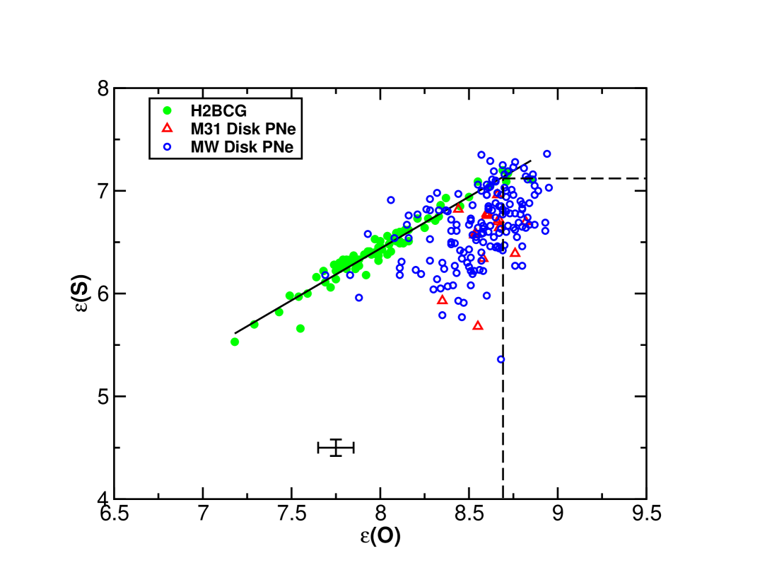
Figure 1: Plot of $\rm\epsilon(S)$ versus $\rm\epsilon(O)$ for a large sample of MWG and M31 disk planetary nebulae (open symbols) along with a sample of H II regions and blue compact galaxies selected from the literature (H2BCG; filled symbols). The solid line is a least squares fit to the H2BCG sample. The dashed lines show solar abundances from Asplund et al. (2009). Average uncertainties for the S and O abundances of the PN sample, determined by propagating line measurement uncertainties through the abundance-determining step, are shown.

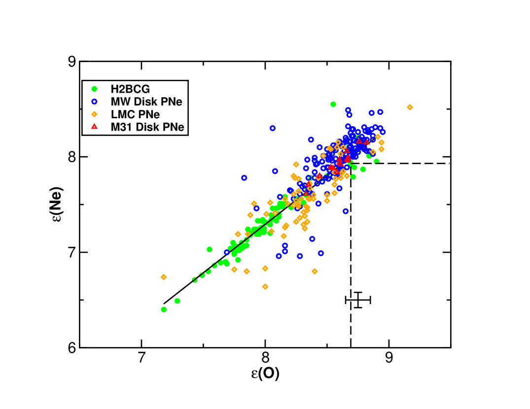
Figure 2: Same as Fig. 1 but for $\rm\epsilon(Ne)$ versus $\rm\epsilon(O)$. We have also added PNe from the LMC.

The sulfur anomaly can be seen clearly in Figure 1, where we have plotted $\rm\epsilon(S)$ versus $\rm\epsilon(O)$ for a large sample of PNe in the disks of the Milky Way and M31 galaxies (open symbols) as well as a combined sample of blue compact galaxies (BCG) and Galactic and extragalactic H II regions (hereafter referred to as H2BCG; filled circles) for comparison purposes. Fig. 2 is an analogous plot of $\rm\epsilon(Ne)$ versus $\rm\epsilon(O)$. In both plots the abundances for the Milky Way PN sample were taken from HKB04, Milingo et al. (2010), and Henry et al. (2010), where data for all objects were obtained, reduced, and measured by the same team of astronomers. In addition, all elemental abundances were recently recomputed using an updated version of the ELSA abundance package (Johnson & Levitt, 2006) and the results compiled into a database by Dr. Karen Kwitter and her students at Williams College. Thus, the final abundances are considered to be homogeneous. Likewise, the M31 PN abundances were taken from Kwitter et al. (2012). In Fig. 2 we have added measurements of 70 LMC PNe from Leisy & Dennefeld (2006). Abundances for the H2BCG comparison sample were taken directly from the literature. The BCG data were taken from Izotov & Thuan (1999). For the H II regions we used abundances in M101 from Kennicutt, Bresolin, & Garnett (2003), from Shaver et al. (1983) for three objects in the MWG, and from Esteban et al. (2004) for the Orion Nebula. The solid line is a least squares fit to the H2BCG sample. Solar abundances from Asplund et al. (2009) are shown with dashed lines.

The difference in behavior between the PN sample and the sample of H2BCG in Fig. 1 is striking. For the latter group, the objects clearly fall along a narrow linear track which extends over roughly two orders of magnitude in metallicity. This lockstep behavior between S and O is expected, since these two elements are alpha elements, synthesized under similar conditions in massive stars. Assuming the existence of a universal initial mass function, the lockstep behavior should be galaxy-independent. As H II region and BCG abundances represent element levels in the ISM of their host systems, their behavior exhibited in Fig. 1 is not surprising.

At the same time, PN abundances reflect not only the level of an element present in the progenitor star at the time that it formed but also any changes to those abundances brought about by nuclear processes occurring within the star during its lifetime. In the specific cases of S and O, there is currently no strong evidence, except perhaps at very low metallicity, that PN progenitor stars alter their initial levels of these two elements (see the extended discussion on this topic in section 5 below), and so their abundances directly reflect the amounts of S and O present in the local ISM when the star formed. Under this assumption, we would expect the lockstep behavior seen in the case of the H2BCG objects to be the same for PNe. As we see in Fig. 1, it is not.

Interestingly, the offset in S abundances between PNe and H2BCGs is not duplicated for neon abundances shown in Fig. 2, i.e., we see no evidence for an offset between the two object types, although PNe continue to show more scatter. Therefore the differences in PN behavior demonstrated in Figs. 1 and 2 suggest that the offset in Fig. 1 is related to sulfur and not oxygen. Analogous plots of S versus either Ne or Ar show that S is always offset from the H2BCGs by roughly the same amount and in the same direction, further emphasizing that the problem resides with sulfur. A similar conclusion is drawn when one inspects the plots of Ne, Ar, and S versus O in Milingo et al. (2010).

In what follows, we carefully examine a large number of potential explanations for the sulfur anomaly. In section 2 we test for correlations between the magnitudes of the vertical offsets of PN sulfur abundances from the H2BCG track in Fig. 1, i.e., sulfur deficits, and numerous independent parameters related to the nebula and/or central star. In section 3 we check on the robustness of the sulfur ionization correction factor (ICF) using standard photoionization models, tests of the relevance of dielectronic recombination, as well as direct measurements of the S⁺³ abundance available in the literature. Section 4 looks at the possibility that S is sequestered in either dust or molecules, while section 5 explores the possibility that the sulfur anomaly results from stellar nucleosynthesis in AGB stars. Our summary and conclusions are provided in section 6.

2 Correlation Tests Involving Nebular and Stellar Properties

Table 1 lists the results of correlation tests performed on our PN database. We define the sulfur deficit $\rm SD\equiv\epsilon(S_{exp})-\epsilon(S_{icf})$, where $\rm\epsilon(S_{exp})$ is the expected S abundance, i.e. the abundance that a PN of a given O abundance would possess if its S abundance placed it on the H2BCG track, while $\rm\epsilon(S_{icf})$ is the S abundance of a PN inferred with the use of an ICF. Thus the more that a PN is displaced below the H2BCG track the more positive the $\rm SD$ value. For each test the sulfur deficit was plotted against one of the 24 separate independent parameters listed in column 1 for the number of objects in column 2. The variables tested, from top to bottom in column 1, are: reddening factor, log of the ion ratio, oxygen ionization correction factor, sulfur ionization correction factor, log of the nebular diameter, central star mass, log of the central star’s luminosity, neon deficit (defined in the same way as the sulfur deficit), log oxygen abundance, log of the ion ratios (4 rows), log of the difference between a PN’s measured O abundance and the ambient interstellar abundance at its location along the disk, the PN’s galactocentric distance along the disk, electron temperatures derived from the lines indicated (next five variables), electron densities based on the lines indicated (next two variables), and excitation class based upon the indicated emission lines and employing expressions for excitation class developed by Dopita & Meatheringham (1990).

Column 3 displays the value of the Pearson correlation coefficient, while column 4 lists the correlation probability, i.e., the probability that the correlation could have resulted by choosing the same number of objects from a completely uncorrelated parent population. Defining r=0.6 as the minimum value for a likely correlation (our justification of this is explained in Appendix A), all but one of the tests indicate the absence of a correlation. The exception is the relation between the SD and $\rm\log(S^{+3}/S^{+2})$. The increase of this ratio with the SD suggests that the deficit is due in part to the failure of sulfur ICFs to correctly account for the higher ionization stages of sulfur. Interestingly, we see no significant correlation between the SD and either the $\rm Ar^{+4}/Ar^{+3}$ or $\rm Ar^{+3}/Ar^{+2}$ ratios. The ionization potentials of S⁺² and S⁺³ are 34.8 eV and 47.2 eV, while those of $\rm Ar^{+2}$ and $\rm Ar^{+3}$ are 40.7 eV, and 59.8 eV, respectively. Since we see no significant correlation for $\rm Ar^{+3}/Ar^{+2}$, this suggests that there should be little sulfur in stages above S⁺³. If the sulfur anomaly is the result of underestimating the population of ionization stages above S⁺², it appears that the only significant stage in this case would be S⁺³. We conclude that, with the exception of $\rm\log(S^{+3}/S^{+2})$, none of the other factors listed in Table 1 is significantly related to the sulfur anomaly. We should point out, however, that the question of a link between sulfur deficit and PN morphology was not explored. Such a study should perhaps be undertaken in the future.

3 Evaluating the Effectiveness of the Sulfur Ionization Correction Factor

The ionization correction factor is the ratio of the elemental abundance to the total of the observed ionic abundances. It corrects for the unobservable ions of an element. In the case of sulfur, normally only the S⁺ and S⁺² ions are directly observable, although we know from photoionization models that higher stages, e.g., S⁺³, are present in PNe in significant quantities. ICFs are usually based upon nebular models from which the abundances of the unseen ions can be estimated. It is therefore natural to speculate that the observed PN sulfur deficits are due to a formulated ICF for sulfur which incorrectly adjusts for the unseen ions.

Various formulas for the sulfur ICF have been developed over the last four decades, including those of Peimbert & Costero (1969), Stasińska (1978), French (1981), Kingsburgh & Barlow (1994), and Kwitter & Henry (2001). With the advent of ISO and Spitzer, however, the S⁺³ ion has been observed directly in over 30 PNe in which oxygen abundances were also reported by Pottasch & Bernard-Salas (2010). These observations have lessened the need of an ICF in these PNe and allowed for the more direct computation of the S abundance, although the sulfur deficit problem has not been discussed extensively in the context of these observations.

In this section we check to see if photoionization models, from which ICFs are derived, reproduce the sulfur deficits observed in three sample PNe. We also test the relevance of dielectronic recombination and the possibility that incorrect rates could produce flawed ICFs. Finally, we report on the implications that direct IR measurements of S⁺³ have for the sulfur deficits.

3.1 Photoionization Models

3.1.1 Standard Models

The abundance analysis by HKB04 of their PN sample included the calculation of photoionization models of three PNe representing a large range in the sulfur deficit, i.e., IC 4593, Hu 2-1, and NGC 3242. The program CLOUDY (Ferland et al., 1998) was used along with input blackbody stellar SEDs to model each object’s measured line strengths. In the process, elemental abundances, which comprised part of the model input information, were adjusted along with other parameters such as gas density and central star temperature and luminosity in order to produce a list of predicted line strengths which closely matched the observed values. [Since then, the sulfur abundance of NGC 3242 has been revised and a new model of that PN was recently calculated by Matthew Hosek at Williams College using a central star SED of 91,000 K from Rauch (1997). Results of the new model are used in this discussion.] Table 2 provides a comparison of empirical and model O and S abundances along with associated sulfur deficits. We see that the model abundances for O and S along with the resulting sulfur deficit agree well with the analogous values inferred from observations for each of the three PNe used in this analysis.

Clearly the fact that models and observations agree closely suggests that either standard models should not be used to derive sulfur ICFs, or the sulfur ICF is correct and there is a real gas-phase sulfur abundance deficit in these nebulae. In the former case, some S may be sequestered in ionization stages whose populations are underestimated by the models for reasons that are unknown at this time. Next, we consider possible effects of dielectronic recombination on the ionization structure of S in model nebulae, and by extension, the ICF for sulfur.

3.1.2 Dielectronic Recombination

Many of the sources of atomic data used in the photoionization code CLOUDY are summarized in Ferland et al. (1998) with updates on the Cloudy web site www.nublado.org. Could uncertainties in the atomic data produce the sulfur anomaly discussed here?

The ionization balance of hydrogen and helium are quite reliable, since the ionization and recombination of these elements is dominated by valence shell photoionization and radiative recombination. These processes are discussed, for instance, in Osterbrock & Ferland (2006, Chapter 2).

The situation is complex and more uncertain for the heavy elements. Ionization for a PN is predominantly by valence shell photoionization, although inner shell photoionization and Auger decay can be significant (Osterbrock & Ferland, 2006, Chapter 11). The heavy elements primarily recombine through dielectronic recombination, a process where a free electron is captured into autoionizing levels. These are levels with two excited electrons and with energies above the ionization limit of the recombined atom (Osterbrock & Ferland, 2006, Appendix A4). These rates of dielectronic recombination (DR) are sensitive to the energies of the autoionizing levels because they determine whether free electrons can reach those levels. In practice, accurate DR rates require experimental autoionization level energies.

For high gas temperatures, we use the recombination data set collected by Nigel Badnell for both radiative and dielectric recombination. DR rates are available for elements of the second row (O and Ne are important for optical spectra of PN) but only for relatively high ions of the third row. In particular, experimental energies are not available for the low ions of sulfur studied in this paper, and their sulfur DR rates are not given by Badnell. Instead, for these ions we use estimates of the rates based on the simple averaging approach described by Ali et al. (1991). That is, the Badnell rates are joined on to the mean of charge-specific CNO rates at lower temperatures.

It is impossible to say how uncertain these estimates might be. Comparing with other ions this method generally works to within a factor of two. Could such uncertainties affect the ionization balance and line emission enough to cause models to misrepresent what happens in real nebulae? We vary the estimated DR rate by these amounts to find out.

In the present case, we investigated the effects of varying the DR rate on sulfur emission line strengths as a way of identifying a mechanism which could profoundly affect the ICF of sulfur in a way that would explain the observed sulfur deficits. For example, overestimated rates would affect the sulfur ionization balance by shifting sulfur into lower stages, causing an ICF based on these models to underestimate the sulfur elemental abundance. An opposite shift would result if rates used are below their actual values.

We therefore computed three grids of photoionization models using CLOUDY 08.01, where input parameter ranges for each grid were designed so that the output predicted line strengths spanned the space of observable line ratios for the PN sample. Three model input parameters were varied: the SED of the central star, the overall metallicity, and the nebular gas density. For stellar temperatures between 30,000 and 50,000 K we used the Atlas SEDs by Kurucz (1991), while for temperatures above 50,000 K we employed the SEDs of Rauch (1997). For each grid, input stellar temperature ranged from 30,000-158,000 K, total gas density from 10²-10⁵, and metallicity from 0.25-2.5 times solar. The DR rates in the first grid were the same as those prescribed by Badnell (1991). For the other two grids, the rates were halved or doubled. All models were radiation bounded.

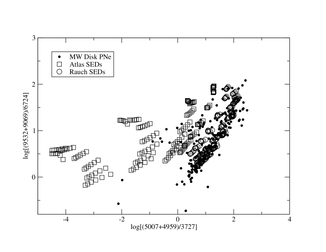
Figure 3: Logs of the [S III]/[S II] and [O III]/[O II] ratios plotted against each other for the same observed MW disk PN sample displayed in Fig. 1 (filled circles) and photoionization models using Atlas (open squares) or Rauch AGB (open circles) input SEDs.

Results for the first grid are shown in Fig. 3, where for each model we computed the predicted line strength ratio of ([S III] $\rm\lambda$9523+$\rm\lambda$9069)/[S II] $\rm\lambda$6724 and ([O III] $\rm\lambda$5007+$\rm\lambda$4959)/[O II]$\rm\lambda$3727. Predicted ratios for models employing the Atlas or Rauch SEDs are shown with open squares and circles, respectively, while the line ratios for the same MW disk PN sample shown in Fig. 1 are shown here with filled circles. First, we note that these models mostly span the space occupied by the observations. The exceptions appear to be the objects with low [S III]/[S II] ratios along with a few with high [O III]/[O II] ratios. In the first case, the observed reduced sulfur ratios are likely the result of partial telluric absorption of the near IR lines at $\rm\lambda\lambda$9069,9532. The second group is more difficult to characterize. However, in comparing a number of their observed properties with those of the majority of the sample, all members of the high [O III]/[O II] group are likely to be matter bounded. For example, compared with the rest of the sample, these objects all possess relatively low observed values of [O I] $\rm\lambda$6300, [O II] $\rm\lambda$3727, and [N II] $\rm\lambda$6584, i.e., lines typically reduced in strength relative to those produced by higher ionization stages when the nebula is matter bounded.

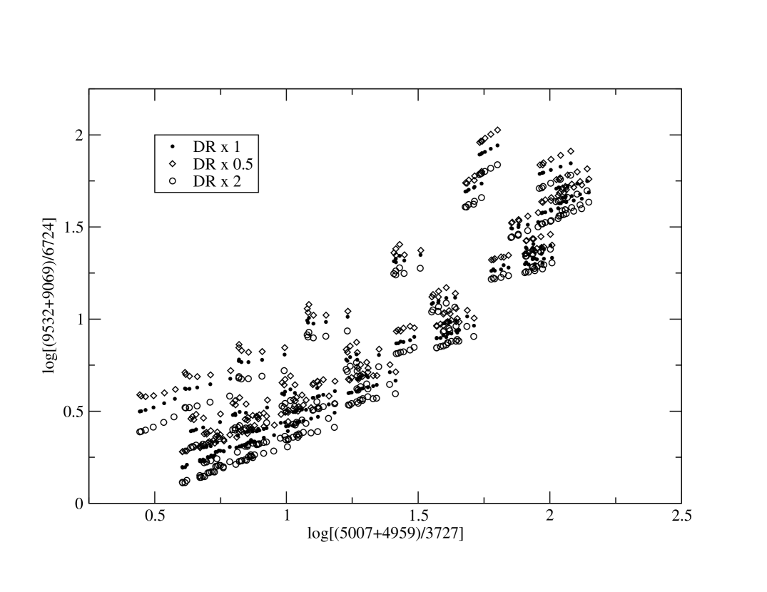
Figure 4: Logs of the [S III]/[S II] and [O III]/[O II] ratios plotted against each other for photoionization models only, using the standard DR rates (closed circles), one-half the standard rates (open diamonds), and twice the standard rates (open circles).

Figure 4 demonstrates the effects of multiplying the Badnell DR rates by factors of 0.5 and 2. Here we plot results for the same line ratios as in Fig. 3 for all three grids. Only the models employing the Rauch AGB SEDs are shown. The figure clearly shows the effects of changing the rates. Typically the model points shift up by about 0.1 dex when the rate is halved and down by a similar amount when the rate is doubled, the directions of the shifts being in the sense that is expected. The thermostat effect, where changes in the abundance of an ion do not linearly affect its emission lines due to energy balance, accounts for the relatively modest change in line emission, despite large changes in the assumed DR rates. Shifts are similar for those models based upon the Atlas SEDs. These changes in DR rates, representing reasonable uncertainties in their actual values, correspond to shifts in the sulfur ICF of about 13% or 0.05 dex above or below the value obtained before DR scaling. Clearly, these small changes in the ICF cannot explain the sulfur anomaly.

3.2 Direct Infrared Observations of S⁺³

All of the sulfur abundances shown in Fig. 1 result from applying an ICF to the observed abundances of S⁺ and S⁺². Does replacing the ICF by directly measuring S⁺³ reduce or eliminate sulfur deficits?

Sulfur abundances of 32 Galactic PNe determined through direct observations of S⁺³ have been summarized by Pottasch & Bernard-Salas (2010). Their study made use of the ISO and Spitzer telescopes to measure the strength of the [S IV] 10.5$\rm{\mu}$m line. Similar measurements using Spitzer were made by Shaw et al. (2010) of six PNe in the SMC and by Henry et al. (2008) of DdDm-1, located in the Galactic halo.

In Table 3 we provide S abundance results which have been derived using both the ICF method ($\rm S_{icf}$) and the IR method (S_ir). For each object identified in the first column we list in columns 2-5 the values for $\rm\epsilon(O)$; $\rm\epsilon(S_{exp})$, i.e., the $\rm\epsilon(S)$ value on the H2BCG track for the given oxygen abundance; $\rm\epsilon(S_{icf})$; and $\rm SD_{icf}$. For the last quantity we have added the subscript to indicate that it is based on the standard ICF abundance method. Columns 6 and 7 give $\rm\epsilon(S_{ir})$ resulting from the IR measurements and the associated sulfur deficit SD_ir based upon values in column 3. Column 8 provides a measure of the difference in S abundances derived from the two methods. Finally, values in column 9 represent the amount of an unidentified ion of S such as S^o or S⁺⁴, relative to S_exp, needed to explain the difference between $\rm S_{ir}$ and $\rm S_{exp}$, i.e., $\rm S^{i}/S_{exp}=1-\log^{-1}(-SD_{ir})$.

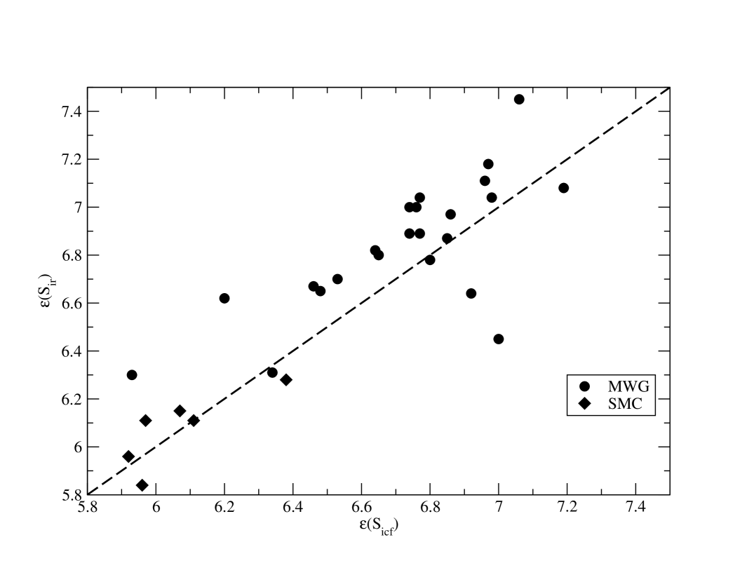
Figure 5: Sulfur abundances inferred from IR data versus S abundances derived using an ICF. Filled circles and diamonds show positions for PNe in the MWG disk and the SMC, respectively. The dashed line shows the one-to-one correspondence.

Fig. 5 shows a visual comparison of the $\rm\epsilon(S_{ir})$ and $\rm\epsilon(S_{icf})$ values in Table 3, where Milky Way disk objects appear as filled circles, SMC objects as filled diamonds. The dashed line indicates the one-to-one correspondence. With a few exceptions there is a clear tendency (21 of 29 objects) for the IR abundances to exceed the corresponding ICF abundances. Of those 21 PNe the median positive vertical distance from the line is 0.17 dex or a factor of 1.5 times the $\rm S_{icf}$ value. This suggests that when S⁺³ observations replace the ICF method, half again as much S, on average, is inferred. This result is qualitatively consistent with the positive correlation we found in § 2 between the SD and $\rm\log(S^{+3}/S^{+2})$. For those eight objects falling below the line, apparently the ICF overcorrects for unobserved sulfur ions, as would be the case if these PNe were matter-bounded.

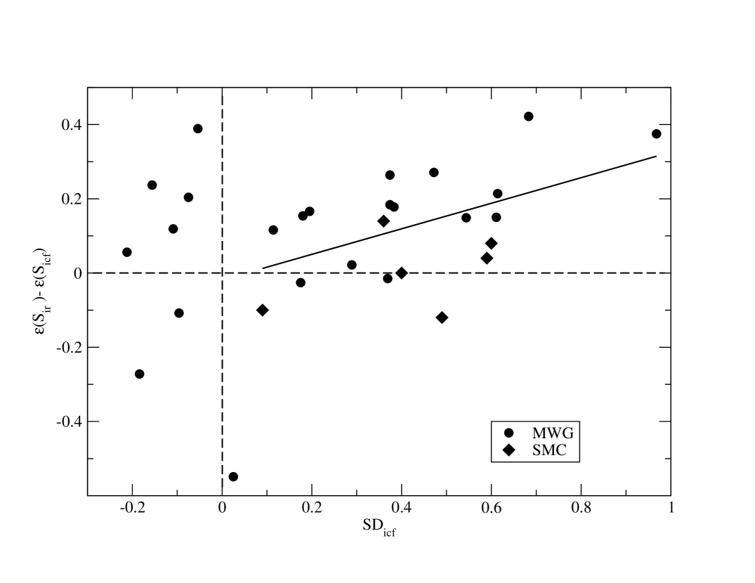
Figure 6: The difference in logarithmic S abundances inferred from IR and ICF methods versus SD_icf. Filled circles and diamonds represent PNe in the Milky Way disk and SMC, respectively. Objects to the right of the vertical dashed line have S abundances which fall below the values on the H2BCG line for their O abundance, while objects to the left of the dashed line have S abundances above that trend line. The horizontal dashed line separates the plot into regions of positive and negative values for $\rm S_{IR}-S_{ICF}$. The solid line shows a least squares fit to the subset points with positive values for $\rm SD_{ICF}$.

Next, if the sulfur deficit is caused by the failure of the ICF method to properly correct for S⁺³, then there should be a direct correlation between the sulfur deficit SD_icf and the quantity $\rm\epsilon(S_{ir})-\epsilon(S_{icf})$. Values listed in columns 5 and 8 of Table 3 are plotted against each other in Fig. 6. For this analysis we focus on those objects with positive values for SD_icf, i.e., those to the right of the vertical dashed line, ignoring the one outlier near the vertical line at the bottom of the plot. Here we see by inspection some evidence for a positive correlation. A regression analysis of the 21 points provides the least squares fit shown by the solid line. The slope of the line is +0.34$\rm\pm$.13 with an intercept of -0.01$\rm\pm$.06 dex. However, the correlation coefficient $\rm r=+0.52$, with a probability of less than 1% that the same set of points could have come from an uncorrelated sample. As explained in Appendix A, most statisticians require a value of $\rm r\geq 0.6$ for a true correlation, and so we conclude that the apparent trend in Fig. 6 is not robust enough to confirm a relation between values in columns 5 and 8.

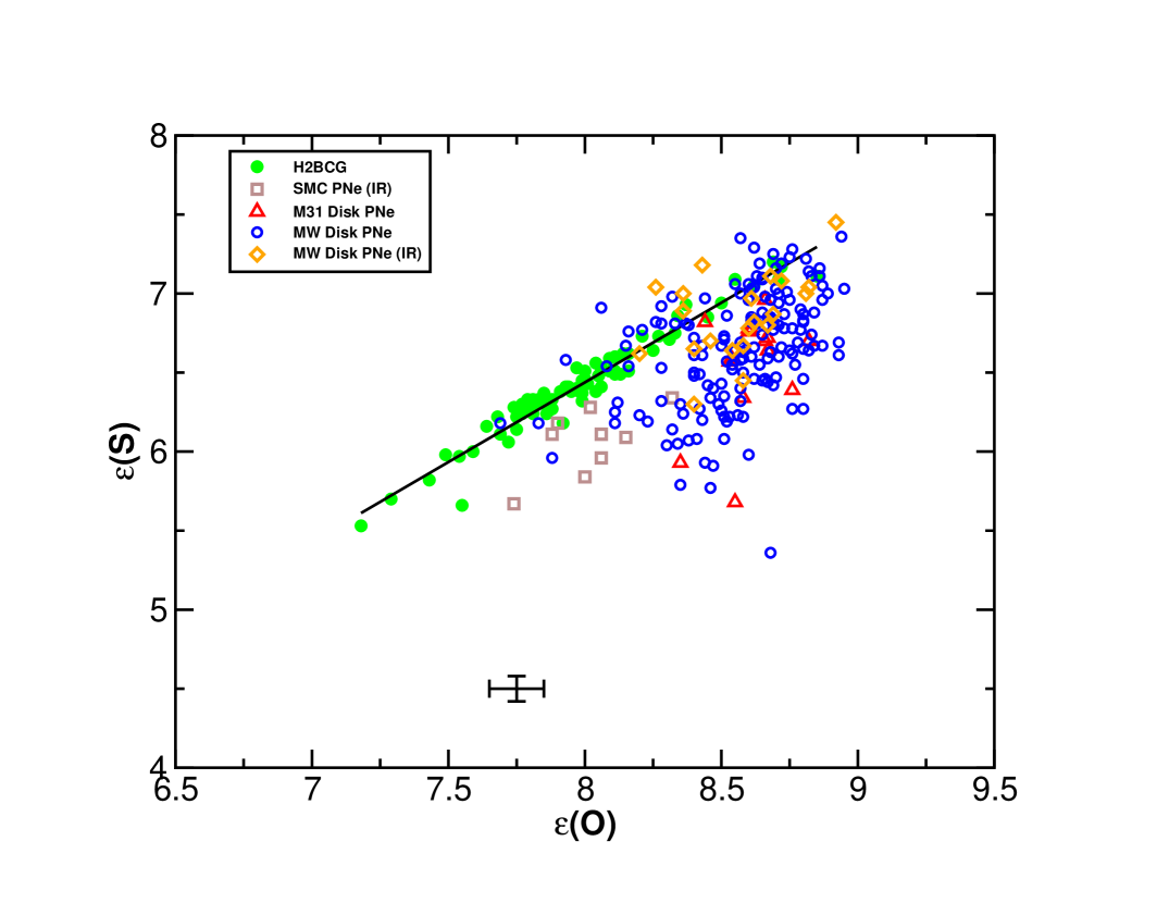
Figure 7: Same as Fig. 1 but now showing the objects from the samples of Pottasch & Bernard-Salas (2010, open diamonds) and Shaw et al. (2010, open squares) in which IR observations were used to infer S abundances.

Approaching this line of investigation regarding S⁺³ from another angle, however, we have added the S and O abundance data from Pottasch & Bernard-Salas (2010, open diamonds) and Shaw et al. (2010, open squares) to the original plot in Fig. 1 to produce Fig. 7. Compared with the original PN sample of open circles, we now see a reduced tendency for these objects to fall systematically below the H2BCG track. Also, the vertical scatter is much closer to what we see in the case of neon in Fig. 2 and perhaps can be attributed simply to natural abundance scatter. Thus, the direct use of the S⁺³ abundances to determine total S abundances seems to solve at least part of the problem related to the sulfur anomaly, as originally anticipated by HKB04. This finding is also consistent with the model results of Gonçalves et al. (2011), who use the 3-D photoionization code Mocassin to show that as the temperature of the PN central star increases, the sulfur ion population shifts upward and the ratio of the sulfur ICF of Kingsburgh & Barlow (1994) to the ’true’ value inferred from the ionization populations in the model output declines.

Shifting attention now to the points in Fig. 6 with negative $\rm SD_{icf}$ values, we see that there is no apparent relation between the parameters plotted. If we speculate that the sulfur anomaly is the result of an unknown nebular property that populates unseen ionization stages of S beyond what we find in the models discussed above, then we can conclude that this same property is not relevant for these seven objects. For them, other factors are influencing the values of $\rm S_{ir}-S_{icf}$, but they appear to be unrelated to the sulfur anomaly.

We turn now to the interpretation of the values posted in the last column in Table 3, i.e., $\rm S^{i}/S_{exp}$ [$\rm=1-\log^{-1}(-SD_{ir})$]. For a given oxygen abundance, if we take S_exp to be the sulfur abundance of a PN falling on the H2BCG track, then the value in column 9 is the fraction of that total abundance that represents the difference between it and the sum of S⁺, S⁺², and S⁺³ measurements, i.e., S_ir. (The six objects with negative $\rm SD_{ir}$ values are irrelevant here.) The average value of $\rm S^{i}/S_{exp}$ is 0.43$\rm\pm$.24. This is rougly the level of the estimated natural scatter inferred from neon abundances of about 0.2 dex or 60% (see Fig. 2). Generally, then, replacing the ICF with direct S⁺³ measurements appears to reduce sulfur deficits in most PNe to the level of expected scatter in the S abundance. However, we note that these objects still fall systematically below the H2BCG track, and thus the deficits of PNe are not entirely explained by employing the direct measurement of S⁺³. This conclusion is consistent with results reported by Bernard-Salas (2006) and Pottasch & Bernard-Salas (2006).

Values in column 9 surpassing this scatter level would suggest that additional ions of S such as S^o and/or S⁺⁴, are present in significant amounts in these objects. We note that an unexpectedly high abundance of ions such as S⁺⁴ in PNe is predicted by nebular models by Jacob (2011) in which the density profile of the nebula is non-uniform. Our standard CLOUDY models suggest that S⁺⁴ has a permitted line S V $\rm\lambda$1198 corresponding to the 3s3p ³P to 3s^{2 1}S₀ transition. If we assume an ion fraction of 10% for S⁺⁴, then, extrapolating from these same model predictions, the S V line will be well below detection levels. Note, however, that considerations of ion ratios and ionization potentials in § 2 appear to conflict with the idea of significant abundances of ions above S⁺³.

4 Dust and Molecules

In studies of the ISM, deficiencies in the abundances of elements in atomic (or ionized) gas is usually assumed to be due to depletion into dust grains (e.g. Whittet, 1992; Krugel, 2008). Consequently, the observed sulfur deficit in PNe has been attributed to sequestration into dust grains (Bernard-Salas et al., 2008). The chemical composition of dust in PNe should reflect that of their parent Asymptotic Giant Branch (AGB) stars. The atmospheres of AGB stars are expected to change as these stars evolve, due to convective dredge up of carbon produced in the He-burning shell. The amount of carbon relative to oxygen (the C/O ratio) is critical in determining which types of dust and molecules are present around an AGB star. The formation of extremely stable CO molecules will consume whichever of the two elements is less abundant, leaving only the more abundant element available for dust formation. Stars start their lives with the cosmic C/O ratio of $\rm\approx$0.4 and are therefore oxygen-rich. In about a third of AGB stars, enough carbon will be dredged up to make C/O $\rm>$ 1 and therefore carbon will dominate the chemistry around these stars.

Sulfur-bearing solids (e.g. MgS, CaS and FeS) are predicted to form in carbon-rich environments (e.g. Nuth et al., 1985; Lodders & Fegley, 1995) and have been tentatively observed in carbon-rich AGB stars, PPNe and PNe, e.g. the “30 $\rm\mu$m” feature oftentimes associated with MgS (e.g. Goebel & Moseley, 1985; Nuth et al., 1985; Omont et al., 1995; Begemann et al., 1994; Hony, Waters, & Tielens, 2002).

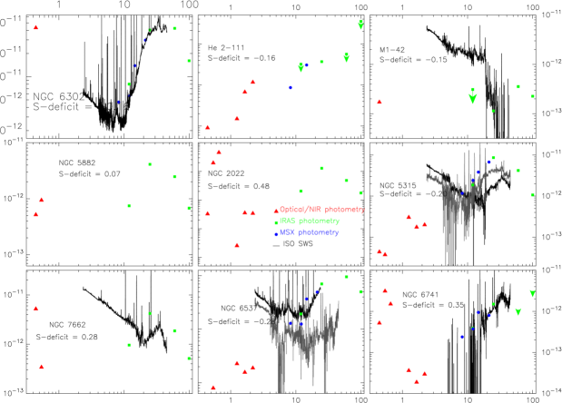
Figure 9: Spectral energy distributions for oxygen-rich PNe. $\rm x$ axis is wavelength in $\rm\mu$m; $\rm y$ axis is $\rm\lambda$ $\rm F_{\lambda}$ in W m^-2; filled triangles are the optical and near-IR photometry (collected from Simbad); filled squares are IRAS photometry; filled circles are MSX photometry; and solid line is the ISO SWS spectrum. Arrows indicate an upper limit on the photometry points. The S-deficit is indicated in the legend for each SED.

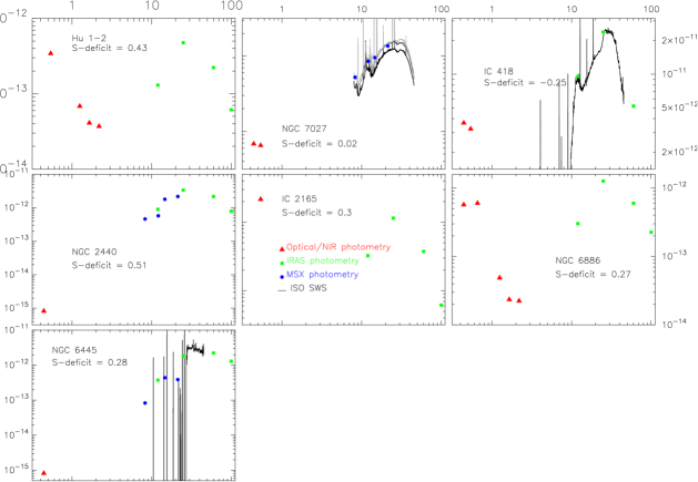
Figure 10: Spectral energy distributions for carbon-rich PNe.

In oxygen-rich environments sulfur-rich grains are precluded by the abundant free oxygen, which will tend to oxidize any sulfides that form, releasing the sulfur back to the gas phase. Therefore, we should expect sulfur depletion in the gas phase to be highest in carbon-rich nebulae. Fig. 8 shows that the distribution of sulfur deficits does not correlate with the the carbon abundance (the determination coefficient r² is 0.202 or r=0.45; see Appendix A for a brief discussion of correlation coefficients.) The figure shows that oxygen-rich PNe possess the same spread in sulfur deficits as their carbon-rich counterparts. Furthermore, there is no correlation between the sulfur deficit and the occurrence of the “30 $\rm\mu$m” feature; some carbon-rich PNe which exhibit the “30 $\rm\mu$m” dust spectral feature also show low sulfur deficits or even enhanced sulfur abundances. Figures 9 and 10 show the spectral energy distributions for a selection of oxygen-rich and carbon-rich PNe, respectively. Although ISO SWS spectra are not available for all objects, it is clear that, for instance, NGC 7027 exhibits a “30 $\rm\mu$m” feature but is barely sulfur-deficient (SD = 0.02); while IC 418, which is enriched in sulfur (SD = $\rm-$0.25), also has a strong “30 $\rm\mu$m” feature.

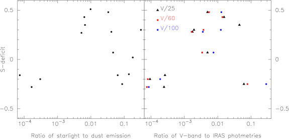
Figure 11: The ratio of starlight to dust emission as a function of sulfur deficit. Left panel the ratio of starlight to dust emission is determined by calculating the area under each hump in the SED for each nebula. Right panel the ratio of starlight to dust emission is estimated using the V-band photometry as a proxy for starlight, and the IRAS 25, 60 and 100 $\rm\mu$m photometries as proxies for dust emission. In both cases $\rm x$-axis is the ratio of starlight to dust emission; the dustiness of the nebulae increases to the left. $\rm y$-axis is the S-deficit.

If sulfur-bearing dust does not exhibit spectral features (only contributes to continuum) and can exist in an O-rich environment, we would still expect to see a correlation between the dust abundance and the sulfur deficit. This is not the case. PNe typically show double-humped SEDs, with a short-wavelength hump due to starlight and a long-wavelength hump due to dust emission. Examination of the SEDs presented in Figures 9 and 10 show that there is no correlation between the S-deficit and whether starlight or dust emission dominates the SED. In order to quantify the ratio of starlight to dust emission we have determined the flux contained in the starlight and dust emission humps by interpolating between the photometry points and calculating the flux beneath each hump. The ratio of starlight to dust emission as a function of sulfur-deficit is plotted in Figure 11.

In some cases, the photometry measurements available are sparse (e.g. IC 2165), which makes the determination of the starlight to dust emission ratio uncertain. Consequently Figure 11 also contains the ratio of the V-band photometry to that in the infrared for the 25, 60 and 100 $\rm\mu$m IRAS photometry - as these far-IR photometry points should be good proxies for dust emission strength. We cannot find any correlation between dust emission and the sulfur-deficit and thus we rule out dust formation as the source of the sulfur abundance anomaly.

Another potential sink for atomic/ionized sulfur gas is molecule formation. Like dust grains, molecules form during the AGB phase. Sulfur-bearing molecules observed around AGB stars include SO, SO₂, H₂S, CS and SiS (Omont et al., 1993; Bujarrabal et al., 1994), and can exist in both C-rich and O-rich environments. As the star evolves towards the PN phase, the molecules will be destroyed by the increasingly high energy photons emanating from the star. However, molecules can survive in highly evolved PNe (e.g. the Helix Nebula; Matsuura et al., 2009, and references therein) as long as they are shielded from the high energy photons by dust (possibly in clumps). Sulfur-rich molecules will not return their sulfur bounty to the gas if the dust shields them. In this case we would still expect to see a correlation between the dust abundance and the sulfur depletion. As shown above (Figures 9 and 10), this is not the case. However, dust emission in clumpy nebulae (like the Helix Nebula) is weak even though the presence of dust is inferred from the survival of molecular species.

In order to test the hypothesis that sulfur can be sequestered in molecules in clumpy nebulae we sought correlations between the ratio of ionized/molecular mass in PNe with the sulfur deficit (Figure 12). The ratios of molecular to ionized gas are taken from Huggins & Healy (1989); Huggins et al. (1996). Unfortunately, the number of PNe for which we have data on both molecular mass and sulfur anomolies is too small to be statistically significant. However, the limited sample in Figure 12 suggests that the highest S-deficit is associated with the lowest molecule content.

We have shown that sulfur abundance anomalies cannot be attributed to sequestration of sulfur into dust grains. Formation and protection of sulfur-bearing molecules may provide a mechanism for sulfur sequestration. Further study of correlations between sulfur abundances and clumpiness of the host nebulae, and with evolutionary status of the nebulae are required.

5 Nucleosynthesis in Asymptotic Giant Branch stars

The illuminated PN is comprised of material from the deep convective envelope, hence nebular abundances should reveal information about the efficiency of mixing events and chemical processing that took place during previous evolutionary phases, in addition to the initial composition of the parent star (Dopita et al., 1997; Karakas & Lattanzio, 2003; Karakas et al., 2009). In light of this information, is it possible to explain the sulfur anomaly in PNe by examining the observed or predicted nucleosynthesis outcomes from AGB stars? We start with a brief review of AGB evolution and nucleosynthesis.

During the TP-AGB phase the He-burning shell becomes thermally unstable every $\rm 10^{5}$ years or so, depending on the core mass. We refer to Busso et al. (1999) and Herwig (2005) for reviews of AGB evolution and nucleosynthesis. The energy from the thermal pulse (TP) drives a convective pocket in the He-rich intershell, that mixes the products of He-nucleosynthesis within this region. The energy provided by the TP expands the whole star, pushing the H-shell out to cooler regions where it is almost extinguished, and subsequently allowing the convective envelope to move inwards (in mass) to regions previously mixed by the flash-driven convective pocket. This inward movement of the convective envelope is known as the third dredge-up (TDU), and is responsible for enriching the surface in ¹²C and other products of He-burning, as well as heavy elements produced by the $\rm slow$ neutron capture process (the $\rm s$ process). Following the TDU, the star contracts and the H-shell is re-ignited, providing most of the surface luminosity for the next interpulse period. In intermediate-mass AGB stars with initial masses $\rm\gtrsim 4M_{\odot}$ (with core masses $\rm\gtrsim 0.8M_{\odot}$), the base of the convective envelope can penetrate into the top of the H-burning shell, causing proton-capture nucleosynthesis to occur there (hot bottom burning, HBB). The surface composition of the star will be changed owing to the fact that the entire envelope is exposed to the hot burning region a few thousand times per interpulse period. Given the fast evolutionary timescales of post-AGB stars with $\rm M_{core}\gtrsim 0.8M_{\odot}$ (Blöcker & Schoenberner, 1991) it is not clear how many end up illuminated as PNe. For this reason, we will concentrate on nucleosynthesis in lower mass AGB stars.

In low-mass AGB stars the evolution of the composition of the surface layers is primarily affected by the occurrence and efficiency of the TDU. The efficiency of the TDU and the composition of the He-intershell have been shown to vary as a function of the initial mass, metallicity, as well as time during the AGB (Boothroyd & Sackmann, 1988; Karakas et al., 2002; Straniero et al., 2003; Karakas, 2010). Observationally these quantities are not well known but a few general trends can be inferred. At the metallicity of the Galactic disk, the TDU likely occurs in stars with initial masses $\rm\gtrsim 1.5M_{\odot}$; this mass is reduced to $\rm\sim 1M_{\odot}$ at the metallicities of the Magellanic Clouds [with metallicities $\rm\sim 2-5$ times less than solar (Wallerstein & Knapp, 1998)]. Of particular interest for this study is the nucleosynthesis that occurs in the He-intershell. This is harder to determine observationally. The subclass of PG1159 post-AGB stars are H-deficient and show what has been considered to be He-intershell material at their surface (Werner et al., 2009). In these stars, C abundances vary from 15–60% (by mass), and O from 2–20%. There are also trace quantities of other He-shell burning products including Ne ($\rm\sim$2%, probably in the form of ²²Ne) and F. Phosphorous is solar, sulfur has abundances varying from 0.01 times solar to solar, and some PG 1159 stars are also highly deficient in Fe (Werner & Herwig, 2006).

The C and O PG 1159 abundances are in direct contrast to intershell abundances predicted by stellar evolution models of AGB stars (e.g., Karakas, 2010). Standard models predict that He constitutes about 75% (by mass), C roughly $\rm\sim 25$%, and there is about $\rm 1-2$% each of ²²Ne and ¹⁶O. The predicted abundances of F and Ne agree with the abundances measured in PG 1159 stars (Werner & Rauch, 1994; Werner et al., 2005). Ne from the intershell is predicted to increase the surface Ne/O ratio, but only when there is very efficient TDU and this has been predicted to occur in only a narrow mass range ($\rm\sim 2.5-3.5M_{\odot}$ Karakas & Lattanzio, 2003; Karakas et al., 2009). The remarkably constant Ne/O ratio observed in PNe with a wide variety of chemical compositions indicates that in most cases this ratio is not altered during the AGB. This is consistent with the conclusion that most PNe originate from masses $\rm\lesssim 2.5M_{\odot}$. Unlike C, O, and Ne, the abundances of P, S, and Fe are affected by neutron-capture reactions in the He-intershell. Depending on assumptions made about the efficiency of the ¹³C($\rm\alpha$,n)¹⁶O neutron source (see, e.g., Busso et al., 2001; Herwig, 2005), P is predicted to be produced by factors of $\rm\sim 1.5$ to 25 times the solar value, whereas the intershell S abundances are 0.6 to 0.9 times solar depending on the AGB model (Werner & Herwig, 2006; Karakas et al., 2009).

To account for the discrepancy between the observed PG 1159 abundances and the predicted intershell composition, Herwig (2000) adopted AGB models with overshoot into the C-O core, that has a composition which is roughly 50% carbon and 50% oxygen. The inclusion of diffusive convective overshoot at the inner edge of the flash-driven convective pocket during a TP dredges up some of the C-O material and leads to large increases in the C and O abundances in the intershell (Herwig, 2000), in line with the PG 1159 observations. The amount of overshoot applied is still however an uncertain free parameter (Herwig, 2000).

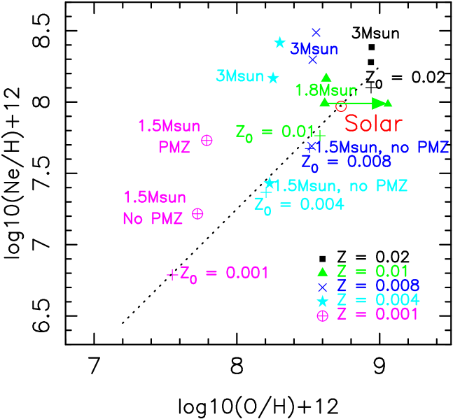
Figure 13: The predicted $\rm\log\epsilon$(O/H) versus $\rm\log\epsilon$(Ne/H) abundances from a selection of AGB models. The composition of the model is sampled from the surface of the star at the very tip of the AGB. The solar composition is shown, and the approximate relationship between O and Ne abundances from HII regions (dotted line). Initial abundances used in the model calculations are shown by the cross symbols for each respective metallicity. The legend shows which symbols correspond to models of a given metallicity. Predictions include: 3$\rm M_{\odot}$, $\rm Z=0.02$ models with and without a partially mixed zone (solid black squares); a 1.8$\rm M_{\odot}$, $\rm Z=0.01$ model with and without a partially mixed zone (solid green triangles); 1.5$\rm M_{\odot}$ and 3$\rm M_{\odot}$ models of $\rm Z=0.008$ (blue diagonal crosses); 1.5$\rm M_{\odot}$ and 3$\rm M_{\odot}$ models of $\rm Z=0.004$ (solid aqua stars); and a 1.5$\rm M_{\odot}$, $\rm Z=0.001$ model with and without a partially mixed zone (magenta circle with cross-hatch). In each case the upper symbol for the same mass corresponds to the model with a partially mixed zone, as these have the highest Ne abundances. We also include results of the synthetic AGB model with an O intershell abundance of 20% (by mass), connected by the arrow to the model with a standard intershell composition (0.8% by mass), see the text for details.

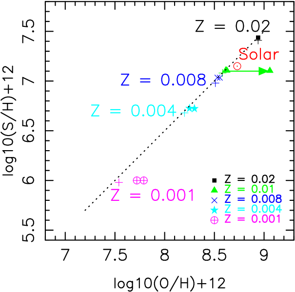
Figure 14: Same as Fig. 13 but for the predicted $\rm\log\epsilon$(O/H) versus $\rm\log\epsilon$(S/H). Here there is no clear distinction between models of different mass or for models with and without a partially mixed zone, except at $\rm Z=0.001$ (where we only include results at 1.5$\rm M_{\odot}$). Also included are results of the synthetic AGB model with an O intershell abundance of 20% (by mass), connected by the arrow to the model with a standard intershell composition (0.8% by mass); see text for details.

Figs. 13 and 14 show the predicted abundances of oxygen, neon, and sulfur from the AGB models [the $\rm Z=0.02,0.008,0.004$ models from Karakas (2010); the $\rm Z=0.01$ model from Karakas et al. (2010); and the $\rm Z=0.001$ model is from Alves-Brito et al. (2011)]. The surface abundances of the AGB models are taken at the tip of the AGB, after the last computed thermal pulse and are taken to be representative of the composition of the envelope when it is ejected from the star. In each figure we show 12+log(O/H) abundances on the $\rm x$-axis versus 12+log(Ne/H) (Fig. 13) or 12+log(S/H) (Fig. 14).

In Fig. 13 we see that there is considerable spread in the Ne abundances predicted from the AGB models. The models that produce the most Ne are those partial mixing zones and those models with masses of $\rm 3M_{\odot}$, which have efficient TDU (Karakas & Lattanzio, 2003). Studies of the $\rm s$-process in low-mass AGB stars suggest that protons need to be partially mixed into the top layers of the He-intershell in order to efficiently activate the main neutron producing reaction ¹³C($\rm\alpha,n$)¹⁶O (e.g., Gallino et al., 1998). In the AGB models shown in Fig. 13 and described for the most part in Karakas (2010), an exponentially decreasing proton profile is introduced into the top $\rm\sim$10-15% of the He-intershell (a partially mixed zone or PMZ). The protons are captured by the abundant $\rm{}^{12}C$ to form a ¹³C pocket (and usually a ¹⁴N pocket), with neutrons released by the ¹³C($\rm\alpha,n$)¹⁶O reaction. The extra Ne production arises from the extra ¹⁴N, which is converted to ²²Ne during convective thermal pulses. From Fig 13 we can see that the effect of this is small at higher metallicities or in lower masses (e.g., the 1.8$\rm M_{\odot}$, $\rm Z=0.01$). The observational data for O and Ne (see Fig. 2) shows some spread, and that most of the lower mass models ($\rm<3M_{\odot}$) fall within that range. Initial mass function considerations, which favor lower mass stars, together with these predictions suggest that the majority Galactic disk PNe evolved from stars of $\rm\lesssim 2M_{\odot}$. There are a few PNe with higher Ne abundances and these may have evolved from higher mass progenitors of $\rm\sim 3M_{\odot}$. At the lowest metallicities shown in Fig. 13 we similarly conclude that most PNe with $\rm\log$(O/H)$\rm<8$ likely have evolved from progenitors less massive than 1.5$\rm M_{\odot}$ and/or did not experience efficient third dredge-up.

In Fig.14 we show the predicted abundances of O and S from the same set of AGB models shown in Fig. 13. In contrast to the predicted spread in Ne, there is no predicted spread in sulfur present in any of the models. We can conclude that AGB models do not result in a net production (or destruction) of S. This is consistent with other AGB calculations (e.g., Forestini & Charbonnel, 1997; Cristallo et al., 2009) and suggests that current AGB models cannot solve the S anomaly problem.

However, the lowest metallicity models show an increase of O and move to the right in the O versus S plot. What if all AGB models, regardless of metallicity, dredged-up sufficient O to move them to the right on the O versus S plot? This could be achieved if convective overshoot from the C-O core increased the O content of the He-intershell as discussed above for PG 1159 stars. In Karakas et al. (2010) the synthetic evolution of a 1.8$\rm M_{\odot}$, $\rm Z=0.01$ model with higher C and O intershell abundances was computed (it was assumed that the neon and sulfur abundance are not changed by this overshoot). In Figs. 13 and 14 we show the results of the synthetic 1.8$\rm M_{\odot}$, $\rm Z=0.01$ AGB model with an O intershell abundance of 20% (by mass), compared to the model with a standard intershell composition (the arrow connects the models and shows the direction caused by the shift in O). This model moves to the right of the line in both figures, and could provide an explanation for the S anomaly.

Is there a need for such overshoot in AGB models? As indicated previously, plots of sulfur versus neon and sulfur versus argon for PNe compared to HII regions show an offset in the sulfur abundance by the same amount compared to the plot of sulfur versus oxygen. This indicates that the problem lies with the sulfur abundances and not with the AGB nucleosynthesis models. However, there are arguments for the inclusion of convective overshoot from the C-O core into the envelope. These are largely based on the composition of the post-AGB PG 1159 stars. These objects are He-rich, likely caused by a late or very late thermal pulse (e.g., Blöcker, 2001). Another supporting piece of evidence is the apparent correlation between oxygen isotope ratios in AGB stars (Harris et al., 1985, 1987). Not only are they correlated with each other but appear to be correlated with the observed carbon and $\rm s$-process element abundances (Harris et al., 1987). Given the large observational uncertainties in the derived oxygen isotope ratios it is difficult to draw firm conclusions (see also Smith & Lambert, 1990). Lastly, the high ¹²C intershell abundances that would result from overshoot into the C-O core changes the neutron exposure and the resulting s-process abundance distribution such that they are no longer consistent with mainstream SiC grains measurements (Lugaro et al., 2003). This suggests that such overshoot is not common in AGB stars that become C and $\rm s$-process rich.

In summary, current AGB models are unable to account for the S anomaly observed in PNe. The inclusion of overshoot from the C-O core into the He-intershell could provide a tentative explanation but only when considering the correlation between O and S. Overshoot does not help clarify the offset present between S and Ne and S and Ar. Furthermore, there are concerns as to the extent of convective overshoot into the C-O during the AGB phase.

6 Summary and Conclusions

The sulfur anomaly is the tendency of planetary nebula sulfur abundances determined from collisionally excited optical line measurements of S⁺ and S⁺² and an ionization correction factor to fall significantly below expected levels. In order to understand its origin, we have quantified the sulfur anomaly by computing a sulfur deficit, i.e., the difference between the observed and expected S abundances, and attempted to relate this value to a broad assortment of other factors relevant to PNe. These include directly measurable properties of the central star and nebula, problems related to determining the contribution of unobservable ionization stages of S to the total elemental abundance (including the effect of inappropriate rates of dielectronic recombination in nebular models used to determine the ionization correction factor for S), sequestration of S into dust and/or molecules, and nucleosynthesis in AGB stars which might either produce S-poor or O-rich material.

Nearly all of these factors can be eliminated from consideration as offering a solution to the problem. We find no evidence that the gap between observed and expected S abundances in PNe is statistically related to any of the 24 nebular or central star properties which we considered with the one exception of $\rm\log(S^{+3}/S^{+2})$ which appears to exhibits a positive correlation. A careful comparison of sulfur deficits and possible IR signatures fails to reveal any indication of sequestration of sulfur into dust or molecules. Likewise for nucleosynthesis scenarios. Using AGB evolution models, we considered in detail if sulfur deficits could be related to either sulfur destruction or oxygen production during the AGB stage of stellar evolution. Here again, we obtained a null result.

The remaining factors which we considered are associated with the sulfur ionization correction factor and the ability to correct for abundances of sulfur ions higher than S⁺². We presented photoionization models of three PNe representing a range in sulfur deficit. The models appeared to be consistent with true gas-phase abundance shortfalls, leaving us with the option of adopting that as the solution or speculating that the models (from which the ICFs are formulated) are failing to account for significant occupation of higher ionization stages. The latter seemed less radical, especially since our consideration of dust/molecules and AGB nucleosynthesis strongly argues against a truly reduced S abundance. Therefore, we further pursued the ICF angle.

We evaluated the impact of under- or overestimated dielectronic recombination rates in altering the sulfur ion population distribution and thereby producing a spurious model-based ICF. We did this by computing large grids of photoionization models in which we tested factor-of-two changes in the rates and compared output line strength ratios with their observed counterparts. We concluded that no reasonable amount of uncertainty in DR rates could explain the sulfur deficits.

Finally, we looked carefully at the PN sulfur abundances derived from direct observation of S⁺³ at 10.5$\rm\mu$m. Having this measurement presumably reduces or eliminates the need to employ an ICF. We were unable to show with statistical certainty that the sulfur deficit for each object correlates with its S⁺³ abundance. On the other hand, a visual comparison of positions in the $\rm\epsilon(S)$ versus $\rm\epsilon(O)$ plane of objects with S abundances inferred from the ICF method and those whose abundances are derived with the IR method show that objects in the latter category generally have smaller sulfur deficits. In fact once the S⁺³ abundances are accounted for, the average size of the remaining deficits for the IR objects resemble the expected size of the abundance scatter, although the deficits themselves are not completely eliminated. It would appear from this part of the analysis, then, that the sulfur deficit is related to the failure of ICFs commonly in use to correct for the true amount of S⁺³ (and possibly higher ionization stages) present in these objects. This notion is supported by the direct correlation we found in § 2 between $\rm\log(S^{+3}/S^{+2})$ and the size of the sulfur deficit. Statistical confirmation of this should follow once additional IR observations are performed. Independent theoretical verification of this point could come from model computations such as those in progress by Jacob (2011). By introducing a negative density gradient into his CLOUDY models, Jacob boosts the relative amounts of the higher ionization stages of sulfur. His approach stands in contrast to the usual use of a constant gas density over the entire nebula, i.e., the common assumption made when using models to infer the form of the sulfur ICF.

Appendix A Correlation Coefficients

When looking for correlations amongst various parameters it is important to define what constitutes a correlation. The strength of a correlation can be measured via the correlation coefficient ($\rm r$). Often it is assumed that any linear regression fit for which r$\rm>0.5$ is an acceptable criterion for a significant correlation (see e.g., Speck et al., 1997; Dijkstra et al., 2005). At the same time Thompson et al. (2006) and Guha Niyogi et al. (2011) define a significant correlation as a set of points for which $\rm r>0.7$ (see also Dijkstra et al., 2005).

The ‘sample correlation coefficient’, $\rm r$, measures both the direction and strength of the relationship between an independent variable $\rm x$ and a dependent variable $\rm y$. The value of the sample correlation coefficent is $\rm-1<r<1$ such that if $\rm r\sim 0$ there is no relationship between $\rm x$ and $\rm y$. The sign ($\rm+$ or $\rm-$) of $\rm r$ merely designates whether the relationship between $\rm x$ and $\rm y$ is positive or negative (i.e. it defines the direction of the slope of the trend.). According to Rumsey (2003), most statisticians like to see $\rm|r|>0.6$ in order to consider a correlation significant, while Thompson et al. (2006) stated $\rm r$ should be $\rm>0.7$, in order to be considered a correlation. For the analysis here we choose the former, $\rm|r|>0.6$.

Table 1: Sulfur Deficit Correlation Tests

Independent Variable	No. of Objects	r	P
c	163	-0.35	3.3E-6
log(He+2/He+)	140	+0.15	0.075
ICFO	161	+0.19	0.015
ICFS	163	-0.024	0.76
log Diameter	101	+0.28	0.004
CPN Mass	95	-0.22	0.030
log L∗	106	+0.11	0.26
Ne Deficit	151	-0.13	0.11
12 + log(O/H)	163	+0.076	0.33
log(O+2/O+)	161	+0.047	0.55
log(S+3/S$\rm{}^{+}2$)	25	+0.60	1.43E-3
log(Ar+4/Ar$\rm{}^{+}3$)	73	-0.067	0.57
log(Ar+3/Ar$\rm{}^{+}2$)	27	+0.29	0.14
log(Oobs-Ograd)	124	+0.38	9.1E-6
Rg(kpc)	124	+0.21	0.018
T(O III)	151	+0.058	0.48
T(O II)	136	+0.0051	0.95
T(S II)	89	+0.053	0.62
T( S III)	147	+0.33	3.44E-5
T(N II)	145	-0.11	0.19
Ne(S II)	147	-0.088	0.29
Ne(Cl III)	65	+0.076	0.54
Excitation Class ($\rm\lambda$5007)	161	+0.11	0.16
Excitation Class ($\rm\lambda$4686)	139	+0.07	0.44

Table 2: Photoionization Models

	Observed			Models
Object	O/H	S/H	SD	O/H	S/H	SD
IC 4593	8.62	6.66	0.42	8.65	6.55	0.56
Hu 2-1	8.43	6.20	0.68	8.39	6.16	0.68
NGC 3242	8.57	7.00	0.02	8.61	6.85	0.22

Table 3: Comparison of ICF and IR Results

Object	$\rm\epsilon(O)$	$\rm\epsilon(S_{exp}$)	$\rm\epsilon(S_{icf}$)	SDicf	$\rm\epsilon(S_{ir}$)	SDir	$\rm\epsilon(S_{ir})-\epsilon(S_{icf}$)	S$\rm{}^{i}/S_{exp}$
SMC
SMP8	7.88	6.33	5.97	0.36	6.11	0.22	0.14	0.40
SMP11	8.02	6.47	6.38	0.09	6.28	0.19	-0.10	0.35
SMP13	8.06	6.51	5.92	0.59	5.96	0.55	0.04	0.72
SMP17	8.21	6.66	6.07	0.60	6.15	0.51	0.08	0.69
SMP24	8.06	6.51	6.11	0.40	6.11	0.40	0.00	0.60
SMP27	8.00	6.45	5.96	0.49	5.84	0.61	-0.12	0.75
MWG
N6210	8.68	7.14	6.85	0.29	6.87	0.27	0.02	0.46
N3242	8.57	7.02	7.00	0.03	6.45	0.57	-0.55	0.73
N6369	8.71	7.16	6.80	0.37	6.78	0.39	-0.02	0.59
N2392	8.28	6.73	6.53	0.20	6.7	0.03	0.17	0.06
IC2448	8.44	6.89	5.93	0.97	6.3	0.59	0.38	0.74
M1-42	8.55	7.01	7.06	-0.05	7.45	-0.44	0.39	$\rm\cdots$
He 2-111	8.44	6.90	6.97	-0.08	7.18	-0.28	0.20	$\rm\cdots$
Hu 1-2	8.43	6.88	6.20	0.68	6.62	0.26	0.42	0.45
IC418	8.28	6.73	6.92	-0.18	6.64	0.09	-0.27	0.18
IC2165	8.40	6.86	6.48	0.38	6.65	0.21	0.18	0.38
MZ3	8.16	6.61	6.76	-0.16	7.00	-0.39	0.24	$\rm\cdots$
N2022	8.80	7.26	6.65	0.61	6.80	0.46	0.15	0.65
N2440	8.62	7.07	6.46	0.61	6.67	0.40	0.21	0.60
N5315	8.64	7.09	7.19	-0.10	7.08	0.01	-0.11	0.03
N5882	8.68	7.14	6.96	0.18	7.11	0.03	0.15	0.06
N6302	8.21	6.66	6.77	-0.11	6.89	-0.23	0.12	$\rm\cdots$
N6445	8.83	7.29	6.74	0.54	6.89	0.40	0.15	0.60
N6537	8.32	6.77	6.98	-0.21	7.04	-0.27	0.06	$\rm\cdots$
N6741	8.79	7.24	6.77	0.47	7.04	0.20	0.27	0.37
N6886	8.65	7.11	6.74	0.37	7.00	0.11	0.26	0.22
N7027	8.52	6.97	6.86	0.11	6.97	0.00	0.12	$\rm\cdots$
N7662	8.55	7.01	6.64	0.37	6.82	0.19	0.18	0.35
DdDm-1	8.06	6.51	6.34	0.18	6.31	0.20	-0.03	0.37

Figure 8: Sulfur deficit versus the observed C/O abundance ratio for those sample objects for which carbon has been measured. The vertical dashed line divides the space between C/O$\rm<$1 (oxygen-rich; triangles) and C/O$\rm>$1 (carbon-rich; circles) environments.

$\rm x$ axis is wavelength in $\rm\mu$m; $\rm y$ axis is $\rm\lambda$ $\rm F_{\lambda}$ in W m^-2; filled triangles are the optical and near-IR photometry (collected from Simbad); filled squares are IRAS photometry; filled circles are MSX photometry; and solid line is the ISO SWS spectrum. Arrows indicate an upper limit on the photometry points. The S-deficit is indicated in the legend for each SED.

Figure 12: The ratio of the molecular gas mass to ionized gas mass as a function of sulfur deficit.

References

- Ali et al. (1991) Ali, B., Blum, R. D., Bumgardner, T. E., Cranmer, S. R., Ferland, G. J., Haefner, R. I., & Tiede, G. P. 1991, PASP, 103, 1182
- Alves-Brito et al. (2011) Alves-Brito, A., Hau, George K. T., Forbes, D.A., Spitler, L.R., Strader, J., Brodie, J.P.., & Rhode, K.L. 2011, A&A, in press
- Asplund et al. (2009) Asplund, M., Grevesse, N., Sauval, A.-J., & Scott, P. 2009, ARA&A, 47, 481
- Badnell (1991) Badnell, N.R. 1991, ApJ, 379, 356
- Begemann et al. (1994) Begemann, B. et al. 1994, ApJ, 423, L71
- Bernard-Salas (2006) Bernard-Salas, J. 2006, in Planetary Nebulae in our Galaxy and Beyond, Proceedings of the International Astronomical Union, Symposium #234. Edited by Michael J. Barlow and Roberto H. M ndez. Cambridge: Cambridge University Press, pp.181-188
- Bernard-Salas et al. (2008) Bernard-Salas, J., Pottasch, S. R., Gutenkunst, S., Morris, P. W., Houck, J. R., 2008, ApJ, 672, 274.
- Blöcker (2001) Blöcker, T. 2001, Ap&SS, 275, 1
- Blöcker & Schoenberner (1991) Blöcker, T. & Schoenberner, D. 1991, A&A, 244, L43
- Boothroyd & Sackmann (1988) Boothroyd, A. I. & Sackmann, I.-J. 1988, ApJ, 328, 671
- Bujarrabal et al. (1994) Bujarrabal, V., Fuente, A., Omont, A., 1994, A&A, 285, 247.
- Busso et al. (2001) Busso, M., Gallino, R., Lambert, D. L., Travaglio, C., & Smith, V. V. 2001, ApJ, 557, 802
- Busso et al. (1999) Busso, M., Gallino, R., & Wasserburg, G. J. 1999, ARA&A, 37, 239
- Cristallo et al. (2009) Cristallo, S., Straniero, O., Gallino, R., Piersanti, L., Domínguez, I., & Lederer, M. T. 2009, ApJ, 696, 797
- Dijkstra et al. (2005) Dijkstra C., Speck A.K., Reid R.B., Abraham P. 2005, ApJ, 633, L133
- Dopita & Meatheringham (1990) Dopita, M.A., & Meatheringham, S.J. 1990, ApJ, 357, 140
- Dopita et al. (1997) Dopita, M. A., Vassiliadis, E., Wood, P. R., Meatheringham, S. J., Harrington, J. P., Bohlin, R. C., Ford, H. C., Stecher, T. P., & Maran, S. P. 1997, ApJ, 474, 188
- Esteban et al. (2004) Esteban, C., Peimbert, M., Garc’ia-Rojas, J., Ruiz, M.T., Peimbert, A., Rodr’iguez, M. 2004, MNRAS, 355, 229
- Ferland et al. (1998) Ferland, G.J., Korista, K.T., Verner, D.A., Ferguson, J.W., Kingdon, J.B., & Verner, E.M. 1998, PASP, 110, 761
- Forestini & Charbonnel (1997) Forestini, M. & Charbonnel, C. 1997, A&AS, 123, 241
- French (1981) French, H.B. 1981, ApJ, 246, 434
- Gallino et al. (1998) Gallino, R., Arlandini, C., Busso, M., Lugaro, M., Travaglio, C., Straniero, O., Chieffi, A., & Limongi, M. 1998, ApJ, 497, 388
- Goebel & Moseley (1985) Goebel, J.H., Moseley, S.H., 1985, ApJ, 290, L35
- Gonçalves et al. (2011) Gonçalves, D.R., Wesson, R., Morisset, C., Barlow, M., & Ercolano, B. 2011, in Planetary Nebulae: An Eye to the Future, Proceedings IAU Symposium No. 283, A. Manchado & L. Stanghellini, eds., Cambridge: Cambridge University Press, arXiv:1110.2709
- Green et al. (2011) Green, J.M., Braxton, K., Balick, B., & Lutz, J. 2011, Bulletin of the American Astronomical Society, Vol. 43, 2011
- Guha Niyogi et al. (2011) Guha Niyogi, S., Speck, A. K., Onaka, T., 2011, ApJ, 733, 93.
- Harris et al. (1987) Harris, M. J., Lambert, D. L., Hinkle, K. H., Gustafsson, B., & Eriksson, K. 1987, ApJ, 316, 294
- Harris et al. (1985) Harris, M. J., Lambert, D. L., & Smith, V. V. 1985, ApJ, 299, 375
- Henry et al. (2010) Henry, R.B.C., Kwitter, K.B., Jaskot, A.E., Balick, B., Morrison, M.A., & Milingo, J.B. 2010, ApJ, 724, 748
- Henry et al. (2008) Henry, R.B.C., Kwitter, K.B., Dufour, R.J., & Skinner, J.N. 2008, ApJ, 680, 1162
- Henry et al. (2004) Henry, R.B.C., Kwitter, K.B., & Balick, B. 2004, AJ, 127, 2284 (HKB04)
- Herwig (2000) Herwig, F. 2000, A&A, 360, 952
- Herwig (2005) Herwig, F. 2005, ARA&A, 43, 435
- Hony, Waters, & Tielens (2002) Hony, S., Waters, L.B.F.M., Tielens, A.G.G.M., 2002, A&A, 390, 533
- Huggins & Healy (1989) Huggins, P.J., Healy, A.P. 1989, ApJ, 346, 201.
- Huggins et al. (1996) Huggins, P.J., Bachiller, R., Cox, P., Forveille, T., 1996, A&A, 315, 284,
- Izotov & Thuan (1999) Izotov, Y.I., & Thuan, T.X. 1999, ApJ, 511, 639
- Jacob (2011) Jacob, R. 2011, Poceedings of IAU Symposium No. 283, Planetary Nebulae: An Eye to the Future, A. Manchado & L. Stanghellini, eds., (Cambridge: Cambridge University Press), in press
- Johnson & Levitt (2006) Johnson, M.D., & Levitt, J.S. 2006, IAU Symposium Series, 234, 439
- Karakas (2010) Karakas, A. I. 2010, MNRAS, 403, 1413
- Karakas et al. (2010) Karakas, A. I., Campbell, S. W., & Stancliffe, R. J. 2010, ApJ, 713, 374
- Karakas & Lattanzio (2003) Karakas, A. I. & Lattanzio, J. C. 2003, Publ. Astron. Soc. Aust., 20, 393
- Karakas et al. (2002) Karakas, A. I., Lattanzio, J. C., & Pols, O.R. 2002, Publ. Astron. Soc. Aust., 19, 515
- Karakas et al. (2009) Karakas, A. I., van Raai, M. A., Lugaro, M., Sterling, N. C., & Dinerstein, H. L. 2009, ApJ, 690, 1130
- Kennicutt, Bresolin, & Garnett (2003) Kennicutt, R.C., Bresolin, F., & Garnett, D.R. 2003, ApJ, 591, 801
- Kingsburgh & Barlow (1994) Kingsburgh, R.L., & Barlow, M.J. 1994, MNRAS, 271, 257
- Krugel (2008) Krugel, E. 2008, “An Introduction to the Physics of Interstellar Dust” Taylor & Francis Group, LLC, New York, p387.
- Kurucz (1991) Kurucz, R.L. 1991, in Proceedings of the Workshop on Precision Photometry: Astrophysics of the Galaxy, ed. A.C. Davis Philp, A.R. Upgren, & K.A. James, (Schenectady: Davis), 27
- Kwitter et al. (2012) Kwitter, K.B., Kehman, E.M.M., Balick, B., & Henry, R.B.C. 2012, ApJ, in preparation
- Kwitter & Henry (2011) Kwitter, K.B., & Henry, R.B.C. 2011, in Planetary Nebulae: An Eye to the Future Proceedings IAU Symposium No. 283, A. Manchado & L. Stanghellini, eds., Cambridge: Cambridge University Press, arXiv:1109.2502
- Kwitter & Henry (2001) Kwitter, K.B., & Henry, R.B.C. 2001, ApJ, 562, 804
- Leisy & Dennefeld (2006) Leisy, P., & Dennefeld, M. 2006, A&A, 456, 451L
- Lodders & Fegley (1995) Lodders, K., Fegley, B., 1995, Meteoritics, 30, 661
- Lugaro et al. (2003) Lugaro, M., Herwig, F., Lattanzio, J. C., Gallino, R., & Straniero, O. 2003, ApJ, 586, 1305
- Matsuura et al. (2009) Matsuura, M., Speck, A.K., Mchunu, B.M. et al. 2009, ApJ, 700, 1067.
- Milingo et al. (2010) Milingo, J. B., Kwitter, K. B., Henry, R. B. C., & Souza, S. P., 2010, ApJ, 711, 619
- Nuth et al. (1985) Nuth, J.A., et al. 1985, ApJ, 290, L41.
- Omont et al. (1995) Omont, A. et al. 1995, ApJ, 454, 819
- Omont et al. (1993) Omont, A., Lucas, R., Morris, M., Guilloteau, S., 1993, A&A, 267, 490.
- Osterbrock & Ferland (2006) Osterbrock, D.E., & Ferland, G.J. 2006, Astrophysics of Gaseous Nebulae and Active Galactic Nuclei–2nd edition, University Science Books
- Peimbert & Costero (1969) Peimbert, M., & Costero, R. 1969, Bol. Obs. Tonantzintla Tacubaya, 5, 3
- Pottasch & Bernard-Salas (2006) Pottasch, S.R., & Bernard-Salas, J. 2006, A&A, 457, 189
- Pottasch et al. (2007) Pottasch, S.R., Bernard-Salas, J., & Roellig, T.L. 2007, A&A, 471, 865
- Pottasch et al. (2008) Pottasch, S.R., Bernard-Salas, J., & Roellig, T.L. 2008, A&A, 481, 393
- Pottasch & Bernard-Salas (2010) Pottasch, S.R., & Bernard-Salas, J. 2010, A&A, 517, A95
- Press et al. (2003) Press, W.H., Teukolsky, S.A., Vetterling, W.T., & Flannery, B.P. 2003, Numerical Recipes in Fortran 77, (Cambridge: Cambridge University Press), pg. 632
- Rauch (1997) Rauch, T. 1997, A&A, 320, 237
- Rodríguez & Delgado-Inglada (2011) Rodríguez, M., & Delgado-Inglada, G. 2011 in IAU Symposium 283, Planetary Nebulae: An Eye to the Future, A. Manchado & L. Stanghellini, eds., (Cambridge: CUP), in press, astro-ph/1109.1861
- Rumsey (2003) Rumsey, D. 2003, “Statistics for Dummies” (Indianapolis: Wiley)
- Shaver et al. (1983) Shaver, P.A., McGee, R.X., Newton, L.M., Danks, A.C., & Pottasch, S.R. 1983, MNRAS, 204, 53
- Shaw et al. (2010) Shaw, R.A., Lee, T-H., Stanghellini, L., et al. 2010, ApJ, 717, 562
- Smith & Lambert (1990) Smith, V. V. & Lambert, D. L. 1990, ApJS, 72, 387
- Speck et al. (1997) Speck A.K., Barlow M.J., Skinner, C.J., 1997, MNRAS, 288, 431.
- Straniero et al. (2003) Straniero, O., Domínguez, I., Cristallo, R., & Gallino, R. 2003, Publ. Astron. Soc. Aust., 20, 389
- Stasińska (1978) Stasińska, G. 1978, A&A, 66, 257
- Thompson et al. (2006) Thompson, G.D., Corman, A.B., Speck, A.K., Dijkstra, 2006, ApJ, 652, 1654.
- Wallerstein & Knapp (1998) Wallerstein, G. & Knapp, G. R. 1998, ARA&A, 36, 369
- Werner & Herwig (2006) Werner, K. & Herwig, F. 2006, PASP, 118, 183
- Werner & Rauch (1994) Werner, K. & Rauch, T. 1994, A&A, 284, L5
- Werner et al. (2005) Werner, K., Rauch, T., & Kruk, J. W. 2005, A&A, 433, 641
- Werner et al. (2009) Werner, K., Rauch, T., Reiff, E., & Kruk, J. W. 2009, Ap&SS, 320, 159
- Whittet (1992) Whittet, D. C. B., 1992, “Dust In The Galactic Environment”, IoP Publishing.