Tree models for difference and change detection in a complex environment

Abstract

A new family of tree models is proposed, which we call “differential trees.” A differential tree model is constructed from multiple data sets and aims to detect distributional differences between them. The new methodology differs from the existing difference and change detection techniques in its nonparametric nature, model construction from multiple data sets, and applicability to high-dimensional data. Through a detailed study of an arson case in New Zealand, where an individual is known to have been laying vegetation fires within a certain time period, we illustrate how these models can help detect changes in the frequencies of event occurrences and uncover unusual clusters of events in a complex environment.

, , and

1 Introduction

We propose a new family of tree models that can be used to uncover distributional differences between multiple data sets. These models, which we call “differential trees,” are suitable for solving sophisticated, multivariate problems. They can be applied, for instance, to change detection and work effectively in an online surveillance fashion.

The research was motivated by a real-world problem. Fire service departments are often interested in detecting changes in the frequencies of different types of fire incidents, automatically from large amounts of data and informatively to shed light on potential causes. This change detection problem is certainly not unique to fire incidents. Similar problems can easily be found in many fields such as climatology, epidemiology and economics.

To investigate the problem in depth, one particular scenario has been chosen as a case study, and is used exclusively in this paper to illustrate and investigate the new methodology. It was known that an individual had been laying vegetation fires between October 2006 and January 2007 in the urban area of Blenheim, New Zealand. The New Zealand Fire Service wishes to be able to automatically detect such a sequence of events as early as possible and isolate them from the rest. At first glance, there seems to be a lack of information to relate the scenario to frequency change detection, since no fire maliciously set by an individual could be definitely known as such in reality. However, a surrogate variable can be used. All fire incidents are categorized by on-the-spot fire fighters as either suspicious or not. Since the maliciously-set fires should be highly correlated to those labeled suspicious, we turn the vaguely-defined practical problem into one of detecting changes in the frequencies of: (a) suspicious and other fires, (b) suspicious fires only, as a more direct approach, or (c) fire incidents of a different categorization, as a less direct approach. We consider the frequency changes as distributional differences.

The problem above poses a number of challenges for traditional change detection methods that rely on parametric assumptions [Basseville and Nikiforov (1993), Gustafsson (2000), Poor and Hadjiliadis (2009)]. For this and similar problems, there may exist a number of potentially relevant variables, which can be either numerical or categorical and may contain missing values. The distribution of fire incidents may depend on many factors, such as geographical, seasonal, time-of-day and day-of-week effects, and is simply impossible to model parametrically. Moreover, an arsonist may operate in certain time periods and in certain neighborhoods, and light fires of certain types.

By contrast, the proposed methodology is particularly suitable for solving such problems. Though belonging to the family of tree models [Breiman et al. (1984), Morgan and Sonquist (1963), Quinlan (1993)], a differential tree is constructed from multiple data sets, as opposed to from a single data set by a conventional method, and purpose-built for difference detection. Intuitively, the method stacks the data sets on top of one another (imagine a two-dimensional case) and then, via recursive space partitioning of tree-structured models, looks for the local areas with heterogeneity. By ignoring variations in individual data sets that are common to all and thus irrelevant to changes, such as geographical and seasonal effects in the arson case, it makes more efficient use of data information than an approach that builds one model from each data set. Hence, it achieves a gain in power which is similar in spirit to that of the paired $t$-test or blocking in experimental design.

Table 1: Variables

Name	Meaning	Values
x	Map grid east	Real
y	Map grid north	Real
Urban	Whether an urban or rural area	$\{1=\mbox{urban}$, $0=\mbox{rural}\}$
Alarm	Alarm method code	$\{1=111$ emergency call, $2=\mbox{exchange}$ phone call, $3=\mbox{running}$ call, $4=\mbox{police}$/ambulance, $5=\mbox{private}$ fire alarm, $6=\mbox{other}\}$
Firetype	Type of fire incident	$\{1=\mbox{structure}$, $2=\mbox{mobile}$ property, $3=\mbox{vegetation}$, $4=\mbox{chemical}$, $5=\mbox{rubbish}$, $6=\mbox{other}\}$
Heatsource	Heat source	$\{1=\mbox{outside}$ fire lit for lawful purpose, $2=\mbox{gas}$/liquid fuelled equipment, $3=\mbox{solid}$ fuelled equipment, $4=\mbox{electrical}$ equipment, $5=\mbox{hot}$ object, $6=\mbox{fireworks}$, $7=\mbox{cigarette}$/smoking materials, $8=\mbox{act}$ of nature, $9=\mbox{exposure fire}\}$
Objignited	Object ignited	$\{1=\mbox{structure}$ component, $2=\mbox{furniture}$/appliances, $3=\mbox{soft}$ goods/bedding, $4=\mbox{decoration}$/recreational materials, $5=\mbox{storage}$ containers and materials, $6=\mbox{electrical}$ equipments/tyres/insulators, $7=\mbox{outdoor}$ items, $8=\mbox{hazardous}$ substances and fuels, $9=\mbox{other}\}$
Time	Time of day	$[0,24)$
day	Day of the quadrennial period	$\{1,2,\ldots,1461\}$
Dayweek	Day of the week	$\{1=\mbox{Monday},\ldots,7=\mbox{Sunday}\}$
label	Category labeled by fire fighters	$\{$suspicious${}={}$suspicious fire, other${}={}$other type$\}$

The arson data used throughout the paper contains information for all fire incidents that occurred within and around Blenheim, a moderately sized town (population 30,200), between 1/Jan/2004 and 31/Dec/2007, as stored in $11$ variables, with names, meanings and possible values given in Table 1. During the quadrennial period, there were a total of $704$ fire incidents, $171$ of which were labeled suspicious. Two variables, heatsource and objignited, contain, respectively, $342$ and $275$ missing values. Pairs of disjoint subsets of the data will be produced in various ways below, and will be used to construct differential trees. Our main focus will be on contrasting the subsets in two biennial periods, 2004–2005 and 2006–2007, to uncover the unusual cluster(s) of fire incidents in the latter period that are likely related to the arson case. We shall also apply the methodology in a sequential detection fashion and compare two consecutive annual periods by shifting time periods progressively. Random subsets will also be produced by permutation or bootstrapping for assessing and enhancing performance.

The rest of the paper is organized as follows. Section 2 briefly reviews the problem of change detection and tree models and gives an overview of the proposed methodology. Section 3 describes in detail the differential tree models and their construction. A primary study of the arson case is presented in Section 4. The performance of the method will be assessed and enhanced in Section 5, with an application in a sequential detection fashion given in Section 6. Section 7 investigates building differential trees using other responses, and Section 8 gives some concluding remarks.

The data and computer code for carrying out the analysis presented in the paper are given in the supplementary material [Wang et al. (2012)].

2 An overview

2.1 Change detection

Change detection has a long history of research in statistics, with a focus on detecting change points [Lai (1995), MacEachern, Rao and Wu (2007), Page (1954), Shewhart (1931)]. These methods, however, rely on parametric assumptions and are applied to situations, such as industrial process control, where such assumptions can be safely made.

Another very useful technique for detecting changes is scan statistics [Glaz, Naus and Wallenstein (2001), Naus (1965)]. This technique looks for unusual clusters of temporal or spatial events in a single data set by using a scanning window to locate clusters of observations that differ in distribution from the rest. Because of the high computational cost, it is only applicable to low-dimensional problems.

2.2 Tree models

Tree models are often used to solve difficult, high-dimensional problems. There are two major families, classification and regression trees, for a categorical and a continuous response variable, respectively [Breiman et al. (1984)]. Other families also exist but are less used, for example, Poisson regression trees for a count response [Chaudhuri et al. (1995), Therneau and Atkinson (1997)] and survival trees for a failure time response with censoring [Davis and Anderson (1989), Ishwaran et al. (2008)].

As in the references above, the basic idea of tree modeling is to partition the space of explanatory variables recursively into increasingly smaller regions so that a simple model fits well to the data in a minimal region. We call such a simple model an atomic model, which can be, for example, the constant function or the normal distribution for a continuous response, or a multinomial distribution for a categorical response, as for regression and classification trees, respectively. A tree model is the composite of the atomic models in the minimal regions and is best represented by a rooted tree, in which a node corresponds to a region, a terminal node a minimal region, and the branching under an internal node a space partitioning. Each internal node thus also has a subtree model.

Building a tree model typically consists of splitting and pruning stages. Splitting proceeds in a top-down fashion, by selecting at each node a split in the form of a logical condition from a large number of candidates, which aims to maximize the homogeneity in subregions. Univariate binary splits are commonly used, for example, $x\leq 3.5$ for a continuous variable, or season${}={}${spring, autumn} for a categorical variable. Splitting continues until homogeneity is reached in a region. An exhaustive splitting is generally beneficial, and allows for uncovering relations hidden deep under the surface. However, a tree grown only by splitting is likely to overfit the data. Hence, it is often followed by pruning, which replaces spurious subtrees with their root nodes in a bottom-up fashion.

Terminal nodes are important for a tree model and the features of interest at those nodes are described by the atomic models. We shall often use the word “pattern” to specifically indicate a terminal node, including its associated region and observations, atomic model, and assessment results.

2.3 Differential trees

In this paper we relate the methodology of tree modeling to difference and change detection. By following the general methodology described in Section 2.2, a differential tree is built from multiple data sets to discover distinguishing patterns between them. Its atomic model is for observations from all data sets, but only the parameters that account for differences in distribution are of direct interest and examined by a homogeneity test. In particular, we will use the Poisson distribution for the count of observations at each level of the response in each data set to form the atomic model, and contrast the event rates in all data sets with a likelihood ratio test of homogeneity.

This new change detection method differs from those described in Section 2.1, in its nonparametric nature and applicability to high-dimensional data. As for other families of tree models, it has the advantages of fast training (relative to most other data mining models), easy handling of different types of variables and dealing nicely with missing values. The resulting models are easily comprehensible, which can be important for change detection, since it helps suggest possible causes behind complicated phenomena.

3 Building differential trees

3.1 A likelihood-based framework

We adopt the likelihood-based approach for building a differential tree and for subsequent analysis. Using the likelihood for tree construction is not rare in the literature, but it sometimes takes an implicit or approximate form. For example, for classification trees the information gain splitting criterion of Quinlan (1993) is equivalent to using the likelihood ratio test, whereas the $\chi^{2}$ criterion [Kass (1980)] and the Gini splitting criterion [Breiman et al. (1984)] are approximations. Su, Wang and Fan (2004) use the likelihood method, in place of the least squares criterion, for building regression trees and obtain simpler yet more accurate tree models in general. Using the likelihood method for tree construction gives results a statistical interpretation, deals with splitting and pruning in one framework, and permits the handling of many families of atomic models in a coherent way. For building differential trees we take one further step, by making use of the $p$-values of the likelihood ratio tests. In general, this helps resolve several difficult issues: (a) splitting in multiple ways; (b) adjusting in the presence of missing values; (c) assessing patterns by their statistical significance; and (d) adjusting for multiple hypothesis testing.

Within this framework, the likelihood ratio test or its statistic can also be conveniently used to assess and compare models, even if there exist nuisance parameters, as in the case of differential trees. We will make extensive use of the fact that the log-likelihood ratio statistic $W$ is asymptotically $\chi^{2}_{\nu}$, with degrees of freedom $\nu$ equal to the number of free parameters for a simple hypothesis or the difference in the number of free parameters for a composite one.

3.2 Likelihood ratio test

The Poisson distribution with probability mass function

$$f(n;\lambda)=e^{-\lambda}\frac{\lambda^{n}}{n!},\qquad\lambda>0,n=0,1,2,\ldots,$$

is widely used to model the number of occurrences of an event over time or in space. Let $Y_{i}$ ($i=1,2$) have the Poisson distribution with rate $\lambda_{i}$. For testing homogeneity

$$H_{0}\dvtx\lambda_{1}=\lambda_{2},$$

the log-likelihood ratio statistic is given by

$$W=2\{\log f(Y_{1};Y_{1})+\log f(Y_{2};Y_{2})-\log f(Y_{1};\bar{Y})-\log f(Y_{2};\bar{Y})\},$$

where $\bar{Y}=(Y_{1}+Y_{2})/2$. Under $H_{0}$, $W$ is asymptotically $\chi_{1}^{2}$.

There are two parameters here, $(\lambda_{1},\lambda_{2})$, or, with reparametrization, $(\lambda_{1},\allowbreak\lambda_{2}-\lambda_{1})$. The focus is on whether $\lambda_{2}-\lambda_{1}=0$, while $\lambda_{1}$ is a nuisance parameter.

3.3 Atomic models

Suppose there are $d$ data sets and the response variable has $c$ levels. For node $\tau$, let $D^{\tau}$ denote the data in its associated subregion, and assume $Y_{ij}^{\tau}$ ($i=1,\ldots,c,j=1,\ldots,d$), the number of observations of level $i$ in data set $j$, is Poisson distributed with mean $\lambda_{ij}^{\tau}$ in that subregion. The atomic model thus has $c\times d$ unknown parameters, $\lambda_{ij}^{\tau}$, or, equivalently,

$$\pmatrix{\lambda_{11}^{\tau}&\lambda_{12}^{\tau}-\lambda_{11}^{\tau}&\cdots&\lambda_{1d}^{\tau}-\lambda_{11}^{\tau}\vspace*{1pt}\cr\lambda_{21}^{\tau}&\lambda_{22}^{\tau}-\lambda_{21}^{\tau}&\cdots&\lambda_{2d}^{\tau}-\lambda_{21}^{\tau}\cr\vdots&\vdots&\vdots&\vdots\cr\lambda_{c1}^{\tau}&\lambda_{c2}^{\tau}-\lambda_{c1}^{\tau}&\cdots&\lambda_{cd}^{\tau}-\lambda_{c1}^{\tau}}.$$

Any nonzero difference in the matrix implies a distributional difference between the data sets. Of direct interest to us is whether all the differences are exactly zero, while those in the first column are nuisance parameters.

We can hence perform a homogeneity test under the null hypothesis

$$H_{0}\dvtx\lambda_{i1}^{\tau}=\cdots=\lambda_{id}^{\tau}\qquad\mbox{for }i=1,\ldots,c.$$ (1)

Letting $\bar{Y}_{i}^{\tau}=d^{-1}\sum_{j=1}^{d}Y_{ij}^{\tau}$ ($i=1,\ldots,c$), the log-likelihood ratio statistic becomes

$$W(\tau;D^{\tau})=2\Biggl{\{}\sum_{i=1}^{c}\sum_{j=1}^{d}\log f(Y_{ij}^{\tau};Y_{ij}^{\tau})-\sum_{i=1}^{c}\sum_{j=1}^{d}\log f(Y_{ij}^{\tau};\bar{Y}_{i}^{\tau})\Biggr{\}},$$ (2)

which is asymptotically $\chi^{2}_{(d-1)c}$ under (1). The test provides evidence for preference between two settings of the atomic model.

As an example, consider the most significant pattern produced by the differential tree shown later in Figure 2. This pattern covers $22$ other and $0$ suspicious fires in the first data set, and $43$ other and $41$ suspicious fires in the second. The test statistic value is

$$W = 2\{\log f(22;22)+\log f(43;43)-\log f(22;32.5)-\log f(43;32.5)\}$$

$${}+2\{\log f(0;0)+\log f(41;41)-\log f(0;20.5)-\log f(41;20.5)\}$$

$$\approx 63.75,$$

which yields a $p$-value of $1.4\times 10^{-14}$ under $\chi_{2}^{2}$.

The appropriate atomic model depends on the problem under study. By assuming equal rates, null hypothesis (1) implies that all data sets were obtained under the same exposure, for example, over time periods of equal length. While this applies to our analysis presented below due to our special partitioning of the data set on an annual basis, one could also consider the case where exposures are different. If the exposures are known, say, $e_{j}$ for data set $j$, one needs to modify $H_{0}$ to

$$H_{0}^{\prime}\dvtx e_{1}\lambda_{i1}^{\tau}=\cdots=e_{d}\lambda_{id}^{\tau}\qquad\mbox{for }i=1,\ldots,c,$$ (3)

where $\lambda_{ij}^{\tau}$ is a rate per unit exposure. Reassigning $\bar{Y}_{i}^{\tau}=\sum_{i=1}^{d}e_{j}Y_{ij}^{\tau}/\sum_{i=1}^{d}e_{j}$, we have

$$W^{\prime}(\tau;D^{\tau})=2\Biggl{\{}\sum_{i=1}^{c}\sum_{j=1}^{d}\log f(Y_{ij}^{\tau};Y_{ij}^{\tau})-\sum_{i=1}^{c}\sum_{j=1}^{d}\log f(Y_{ij}^{\tau};e_{j}\bar{Y}_{i}^{\tau})\Biggr{\}},$$

which is also asymptotically $\chi^{2}_{(d-1)c}$.

If, however, the exposures are unknown, it is impossible to test a null hypothesis of type (1) or (3). Instead, one can investigate if every data set has the same distribution for the proportions of all response levels, namely,

$$H_{0}^{\prime\prime}\dvtx p_{i1}^{\tau}=\cdots=p_{id}^{\tau}\qquad\mbox{for }i=1,\ldots,c,$$ (4)

where $p_{ij}^{\tau}$ is the probability an observation in data set $j$ is of level $i$. Therefore, one can assume that $(Y_{1j}^{\tau},\ldots,Y_{cj}^{\tau})^{\top}$ has a multinomial distribution with probabilities $(p_{1j}^{\tau},\ldots,p_{cj}^{\tau})^{\top}$. The log-likelihood ratio statistic is

$$W^{\prime\prime}(\tau;D^{\tau})=2\Biggl{\{}\sum_{i=1}^{c}\sum_{j=1}^{d}n_{j}^{\tau}\log\hat{p}_{ij}^{\tau}-\sum_{i=1}^{c}\sum_{j=1}^{d}n_{j}^{\tau}\log\hat{p}_{i}^{\tau}\Biggr{\}},$$

where $n_{j}^{\tau}=\sum_{i=1}^{c}Y_{ij}^{\tau}$, $\hat{p}_{ij}^{\tau}=Y_{ij}^{\tau}/n_{j}^{\tau}$ and $\hat{p}_{i}^{\tau}=\sum_{j=1}^{d}Y_{ij}^{\tau}/\sum_{j=1}^{d}n_{j}^{\tau}$. Under $H_{0}^{\prime\prime}$, $W^{\prime\prime}$ is asymptotically $\chi^{2}_{(c-1)(d-1)}$.

Throughout our study, we assume that the underlying distribution of counts is Poisson distributed, and only the null hypothesis (1) and the resulting statistic (2) are used. In general, altering the atomic model alters the family of differential trees being considered, but the framework for analysis remains the same.

3.4 Subtree models

Denote by $T^{\tau}$ the subtree rooted at node $\tau$ and by ${\widetilde{T}}^{\tau}$ the set of its terminal nodes. The log-likelihood ratio statistic for $T^{\tau}$ is given by

$$W(T^{\tau};D^{\tau})=\sum_{t\in{\widetilde{T}}^{\tau}}W(t;D^{t}).$$ (5)

The statistic $W(T^{\tau};D^{\tau})$ is approximately $\chi^{2}$, with degrees of freedom given by the sum of the degrees of freedom of the individual terms.

3.5 Splitting

We only consider univariate binary splits, which use data information most efficiently, allow surrogate splitting in the presence of missing values, and treat numerical variables no differently from ordinal ones. We further turn categorical variables into ordinal ones by using their pre-given order of levels, instead of considering all possible combinations. This avoids the overfitting introduced by level grouping, which can be severe when a categorical variable has many levels. It is also helpful when the pre-given levels are partially ordinal.

Without missing values, the primary split at node $\tau$ is determined by

$$s^{\tau}_{*}=\mathop{\arg\max}_{s\in S^{\tau}}W(T_{s}^{\tau};D^{\tau}),$$ (6)

where $T_{s}^{\tau}$ is the two-child-node tree defined by a univariate binary split $s$ and $S^{\tau}$ is the set of all candidate splits at node $\tau$. For $S^{\tau}$, we consider every explanatory variable and every midpoint between two consecutive distinct values of the variable from all data sets, but we exclude the cases where small subsets (having less than a total of $5c$ observations, by default) are produced. With $s^{\tau}_{*}$, all data sets are split accordingly and the tree is grown with two new child nodes. The splitting process starts with a single node for all data and proceeds in a top-down, recursive style, until a stop-splitting criterion is met, for example, too few observations left.

To find the primary split in the presence of missing values, a slight adjustment is made using $p$-values, which takes account of different sample sizes caused by missing values. For the $k$th variable at node $\tau$, denote by $n_{k}^{\tau}$ the number of observations without missing values and by $p_{k*}^{\tau}$ the smallest $p$-value of all likelihood ratio tests for the $n_{k}^{\tau}$ observations. The adjusted $p$-value is given by

$$\tilde{p}_{k*}^{\tau}=p_{k*}^{\tau}+\gamma\sqrt{p_{k*}^{\tau}(1-p_{k*}^{\tau})/n_{k}^{\tau}},$$ (7)

where $\gamma>0$ is a constant, which is defaulted to $2$ in our implementation. Similar in spirit to the 1-SE rule of Breiman et al. (1984), the adjustment tends to favor variables with fewer missing values.

To determine the correct branch for an observation when the primary splitting variable at a node has a missing value, a surrogate split can be used, as described in Breiman et al. (1984), Section 5.3. A surrogate split is made using a different variable, chosen so that the surrogate split is as similar to the primary split as possible for the observations without missing values. We measure the similarity of two splits by the number of common observations in their resulting subsets. An ordered list of surrogate splits can be constructed according to their similarities to the primary split.

3.6 Pruning

The pruning of an initially grown tree is necessary for removing spurious subtrees. It works in a bottom-up style, by choosing either the atomic model at an internal node or its subtree model. To do this, one could use the cost-complexity measure, which here is just the log-likelihood penalized by the degrees of freedom. For a subtree, it is defined as

$$W_{\alpha}(T^{\tau};D^{\tau})=W(T^{\tau};D^{\tau})+\alpha\operatorname{DF}({\widetilde{T}}^{\tau}),$$

where $\operatorname{DF}({\widetilde{T}}^{\tau})$ is the number of degrees of freedom for all the atomic models in ${\widetilde{T}}^{\tau}$ and $\alpha$ the complexity parameter. Note that the atomic model at a node is just a tree with a single node, so its cost-complexity measure is

$$W_{\alpha}(\tau;D^{\tau})=W(\tau;D^{\tau})+\alpha\operatorname{DF}(\tau).$$

The pruning criterion is as follows:

$$\mbox{Choose the model with the larger value of }W_{\alpha}.$$ (8)

The value of $\alpha$ can be determined by a model selection criterion, such as AIC or BIC, or cross-validation. In principle, replacing a subtree with its root node implies that the event frequencies cannot be further differentiated between the data sets in all subregions.

If the main goal for building a differential tree is to find the most significant differences between data sets, we can simply preserve the most significant patterns in a constructed tree. Let $p_{\min}(\tau)$ be the $p$-value of the hypothesis test performed at the node $\tau$, for example, the likelihood ratio test based on the statistic (2); and $p_{\min}(T^{\tau})$ be the smallest $p$-value of all hypothesis tests performed at the atomic nodes of the subtree $T^{\tau}$. The new pruning criterion is as follows:

$$\mbox{Choose the model with the smaller value of }p_{\min}.$$ (9)

By doing so, each subtree preserves the node with the most significant pattern and keeps it as a terminal node. This also facilitates the $p$-value adjustments, as described in Section 5.1.

In addition, one may set up a threshold $p$-value, say, $p_{\mathrm{cut}}$, such that a subtree is cut off directly if its $p_{\min}(T^{\tau})\geq p_{\mathrm{cut}}$. It helps remove the less significant patterns, while keeping the most significant ones. The tree model may thus be greatly simplified and can be interpreted more easily. In our implementation, we set $p_{\mathrm{cut}}=10^{-6}$ as default. For the arson case study, this roughly corresponds to $p^{\prime\prime}=0.25$; see Section 5.1 for the definition of $p^{\prime\prime}$.

3.7 Pseudo code

To serve as a summary, Algorithm 1 gives the pseudo code of the recursive function that we implemented for building a differential tree from two data sets.

Algorithm 1 Differential Tree Construction (from Two Data Sets)

function difftree($D1$, $D2$)

0:  Data sets $D1$ and $D2$

1:  Create a terminal node $\tau$

2:  Compute $W(\tau;(D1,D2))$ and $p$-value, using (2)

3:  if too few observations in $D1$ and $D2$ then

4:     return $\tau$

5:  end if

6:  Label $\tau$ as an internal node

7:  for each predictor variable do

8:     Find all potential splits from its distinct values in $D1$ and $D2$

9:     Compute $W(T_{s}^{\tau};(D1,D2))$ for each potential split $s$, using (5)

10:  end for

11:  Find the primary split $s^{\tau}_{*}$, using (6) [or (7) in the presence of missing values]

12:  Find all surrogate splits of $s^{\tau}_{*}$

13:  Use $s^{\tau}_{*}$ (and possibly surrogate splits) to partition $D1$ into $(D1_{\mathrm{left}},D1_{\mathrm{right}})$ and $D2$ into $(D2_{\mathrm{left}},D2_{\mathrm{right}})$

14:  $\tau$$left $=$ difftree($D1_{\mathrm{left}}$, $D2_{\mathrm{left}}$)

15:  $\tau$$right $=$ difftree($D1_{\mathrm{right}}$, $D2_{\mathrm{right}}$)

16:  if $\tau$ is preferred over $T^{\tau}$ by (9) then

17:     Discard $\tau$$left and $\tau$$right and label $\tau$ as a terminal node

18:  end if

19:  return $\tau$

4 A primary study of the arson case

4.1 Setup

In this section we compare two approaches to solving the arson problem. Both use label as the response; one utilizes traditional classification trees, and the other builds a differential tree directly. For our case study the latter is more efficient at discovering differential patterns.

We divide the arson data set into two subsets, covering two time periods, 2004–2005 and 2006–2007, respectively (and reset 1/Jan/2006 to day${}={}$1 and similarly the days after). The two subsets contain, respectively, $318$ and $386$ fire incidents, of which $80$ and $91$ are suspicious. Both suspicious and other fires are included in the study, because a maliciously-set fire is not necessarily labeled suspicious or vice versa, and because it illustrates the application of the method to a multiple category problem. In Section 7 we apply the proposed method to detect changes in the frequencies of suspicious fires only, and of fire incidents with a different categorization.

4.2 Two classification trees

To discover differential patterns, let us first consider building two classification trees, one from each subset, and then testing all the patterns induced from a classification tree against the other subset. The rationale is that classification trees, if constructed properly, are consistent estimators of the underlying distributions [Breiman et al. (1984), Chapter 12] and thus their differences are also consistent for estimating the true distributional differences. Note that each individual classification tree is only built to model the underlying relation between the response and explanatory variables for a single data set and thus inevitably may include patterns that are common with the other, for example, for seasonal effects.

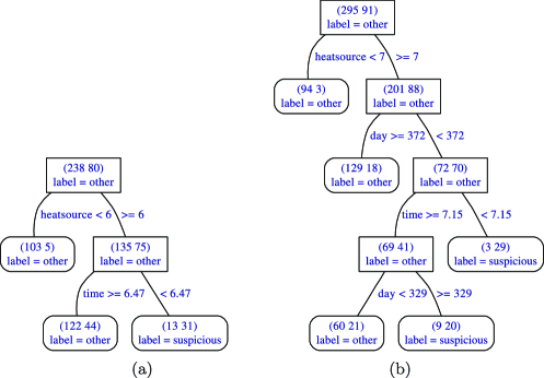
Figure 1: Classification trees built from fire incidents in Blenheim during: (a) 1/Jan/2004–31/Dec/2005 and (b) 1/Jan/2006–31/Dec/2007. Inside the parentheses at a node are the numbers of observations for each response level, here “other” and “suspicious.”

Table 2: Patterns obtained from each of the two classification trees and tested by their covered observations in both subsets

	2004–2005			2006–2007
Pattern	Other	Suspicious	Proportion	Other	Suspicious	Proportion	$\bolds{p}$-value
(a)	Training set			Test set
1	103	05	0.046	090	02	0.022	$3.3\times 10^{-1}$
2	122	44	0.265	183	55	0.231	$1.2\times 10^{-3}$
3	013	31	0.705	022	34	0.607	$2.9\times 10^{-1}$
(b)	Test set			Training set
4	105	07	0.062	094	03	0.031	$3.2\times 10^{-1}$
5	077	38	0.330	129	18	0.122	$3.4\times 10^{-5}$
6	036	17	0.321	060	21	0.259	$3.9\times 10^{-2}$
7	015	00	0.000	009	20	0.690	$4.5\times 10^{-7}$
8	005	18	0.783	003	29	0.906	$2.1\times 10^{-1}$

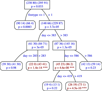
Figure 2: Differential tree built directly by contrasting the fire incidents from 1/Jan/2004–31/Dec/2005 with those from 1/Jan/2006–31/Dec/2007. Each pair of parentheses at a node contains the numbers of observations for all response levels in a data set, and for the arson data here (#other, #suspicious). Any $p$-value less than $10^{-5}$ is marked “***.”

We use the R package “rpart” [Therneau and Atkinson (1997)] for classification tree construction. The classification tree built from the first subset is shown in Figure 1(a). The tree identifies three situations or patterns, as also listed in the upper part of Table 2, in ascending order of their estimated proportions of suspicious fires. To eliminate the patterns that are irrelevant to differences, we test them against the second subset, using (2). Hence, the remaining significant patterns can only be attributed to the distributional differences between the two subsets. After this screening, only pattern 2 remains significant, with a $p$-value of $1.2\times 10^{-3}$. Nonetheless, its significance is mainly due to an increase of “other” in 2006–2007, rather than a change in the frequency of suspicious fires.

Analogously, we can find patterns from the second subset and test them against the first subset. The classification tree built from the second subset is shown in Figure 1(b). It contains five patterns, as listed in the lower part of Table 2. Pattern $7$ is the most significant, with a $p$-value of $4.5\times 10^{-7}$, which corresponds to a remarkable increase of $20$ suspicious fires and appears to be related to the arson case. Specifically, it indicates a significant increase in the proportion of suspicious fires between day 329 (25/Nov/2006) and day 371 (6/Jan/2007), for time after 7:12 am, with heat source that includes cigarettes/matches/candles. It possesses a very different characteristic from pattern 8, which classifies fires as highly suspicious that occur between 0:00 am and 7:12 am, due to heat source${}\geq{}$7. However, with a $p$-value of $0.21$, pattern 8 does not suggest a change, although it merits further investigation by itself. Pattern 5 is also highly significant but corresponds to a decrease of $38-18=20$ suspicious fires, as well as a substantial increase of $129-77=52$ other fires; this change occurred after day 371 (6/Jan/2007).

4.3 One differential tree

A differential tree between the two subsets is constructed, as shown in Figure 2, which contains six terminal nodes. The most significant, with a $p$-value of $1.4\times 10^{-14}$, appears to relate directly to the arson case. Specifically, it suggests that a change has occurred between day 284 (11/Oct/2006) and day 383 (18/Jan/2007), with all types but property fires. The change is due to a substantial increase of $41-0=41$ suspicious fires, as well as an increase of $43-22=21$ other fires. To gain more information about these $41$ suspicious fires, the histograms/barplots for all predictor variables are shown in Figure 3. These fires are exclusively due to heatsource${}={}$7 ($=$cigarettes/matches/candles), mainly of firetype${}={}$3 ($=$Vegetation), largely distributed along a horizontal strip (variable y), and having an increasing trend over time (variable day).

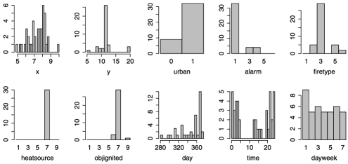
Figure 3: Histograms/barplots for the $41$ suspicious fires covered by the most significant pattern.

The second most significant pattern has a $p$-value of $4.5\times 10^{-10}$ and specifies a situation where there is a decrease in the number of suspicious fires and yet an increase in the number of other fires. This change took place between day 420 (24/Feb/2007) and day 586 (9/Aug/2007).

Note that the general conclusions drawn here are similar to those in Section 4.2. This is not really surprising, since both methods provide consistent estimators for detecting differences between the two underlying distributions. However, we should also notice that the patterns found by the differential tree, that searches for changes directly by ignoring irrelevant patterns, are statistically much more significant [even using the properly adjusted $p$-value (13) or (14)]. This suggests that differential trees are the more efficient approach to change detection. There must therefore be situations where real changes can be detected by the differential tree approach, but not by the other, and especially so when a data set contains many significant patterns not attributable to changes.

5 Performance assessment and enhancement

5.1 Significance adjustment

Since “significant patterns” can always be found with an exhaustive search, one should consider their possible spuriousness. In the following, we consider adjusting $p$-values using the Bonferroni and the permutation method.

The Bonferroni method is the simplest and most conservative. For $m$ tests performed, it adjusts their smallest $p$-value, say, $p$, by

$$p^{\prime}=\min\{mp,1\}.$$ (10)

For building the differential tree shown in Figure 2, there are 13,414 tests performed in total. This includes all candidate splits examined at the splitting stage, including those at the nodes that are cut off later, but not any comparisons at the pruning stage due to their irrelevance in determining the minimum $p$-value. Its adjusted $p$-value for the most significant pattern is thus

$$p^{\prime}=13\mbox{,}414\times 1.4\times 10^{-14}\approx 1.9\times 10^{-10},$$ (11)

which remains highly significant, despite the conservativeness of the method.

The permutation method adjusts a $p$-value by using it as a statistic and is based on the fact that, under the null hypothesis, the adjusted $p$-value has the uniform distribution on $[0,1]$. The $p$-value to be adjusted can be either $p$ or $p^{\prime}$ in (10), and, for the arson data, it does not appear to make much difference. In general, we are inclined to use $p^{\prime}$ since it guards against the situation where an extremely small $p$-value is produced through an exhaustive search. The empirical null distribution can be obtained by permuting either the entire data under investigation, which may nonetheless contain irregular changes and hence reduce the power of detection, or, better, some comparable, “clean” historical data. For the arson case, we choose to permute the entire data here, and later in Section 6 some historical data.

Specifically, our adjustment proceeds as follows. Each observation in the two subsets created in Section 4.1 is randomly reallocated to either the first or second biennial period by tossing a fair coin (without changing its date within a biennial period), thus ensuring the null hypothesis (1) is satisfied. This shuffling destroys all distributional differences between the two periods, but preserves all the relations among the variables such as geographical clusters and seasonal effects. For each pair of random subsets, a differential tree is constructed, and a minimum $p$-value obtained and adjusted by (10). With $R$ ($=$1000 throughout the paper) random replications, $R$ copies of the $p^{\prime}$-value are obtained and ordered into $p^{\prime}_{(1)}\leq\cdots\leq p^{\prime}_{(R)}$, whose self-adjusted values are, respectively, $1/(R+1),\ldots,R/(R+1)$, namely, their expectations under the null hypothesis. Letting $p^{\prime}_{(0)}=0$ and $p^{\prime}_{(R+1)}=1$, a new $p^{\prime}$ can be adjusted by interpolation:

$$p^{\prime\prime}=\frac{j+r}{R+1}\qquad\mbox{if }p^{\prime}_{(j)}\leq p^{\prime}\leq p^{\prime}_{(j+1)},\qquad j=0,\ldots,R,$$ (12)

where $r=(p^{\prime}-p^{\prime}_{(j)})/(p^{\prime}_{(j+1)}-p^{\prime}_{(j)})$.

From the $1000$ differential trees constructed, we obtained $p^{\prime}_{(1)}=8.4\times 10^{-6}$, and, therefore, the permutation adjusted $p$-value for the most significant pattern in the differential tree shown in Figure 2 is

$$p^{\prime\prime}=\frac{1.9\times 10^{-10}/8.4\times 10^{-6}}{1001}\approx 2.3\times 10^{-8}.$$ (13)

This is still an extremely small $p$-value, indicating that it is highly unlikely that this discovered pattern occurred purely by chance.

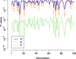
Figure 4: Minimum $p$-values and adjustments in the differential trees constructed from the first $100$, out of $1000$, random permutations of the $4$-year data.

Figure 4 shows the minimum $p$-values from the first $100$ permutations, along with their adjustments. Despite the pure randomness of the permutations, the minimum $p$-values produced by differential trees are remarkably small, indicating the necessity of adjustment. What surprises us most, as can also be seen in results given later, is that $p^{\prime\prime}$ is almost always larger than $p^{\prime}$, because the Bonferroni adjustment is theoretically the most conservative. How could this happen? We think that the reason may lie in the fact that, conditional on the data, patterns with the smallest $p$-values are sought in a deterministic manner, and this has some similarity to a deterministic optimization process, which violates the underlying assumption of randomness for multiple hypothesis testing. If this is true, it has profound implications for many modern statistical methods of modeling and hypothesis testing that involve extensive data manipulation to find the “best” solutions. The bias introduced by such data manipulation may be very high, so high that even the most conservative method can fail to bound it.

5.2 Bootstrap aggregating

One problem with tree models is instability [Breiman (1996b)], which means that a small perturbation in the data may result in a tree with a substantially different structure. In general, an unstable estimator tends to exhibit high variation and low predictive power. For differential trees, this is relevant for discovered differential patterns and their significance levels. Instability, however, can be reduced, often considerably, by using meta-learning techniques, such as boosting [Freund and Schapire (1997)], bagging (bootstrap aggregating) [Breiman (1996a)] or random forests [Breiman (2001)], which resort to building a number of models by perturbing the data. In the following we consider the bagging technique to stabilize the estimation of the minimum $p$-value in a differential tree.

To use bagging on the two subsets described in Section 4.1, we draw a bootstrap sample from each subset and build a differential tree from the pair of bootstrap samples, which gives a minimum $p$-value and its Bonferroni adjustment $p^{\prime}$. This is repeated $B$ ($=$50 throughout the paper) times. The median of the $B$ resulting $p^{\prime}$-values is then taken as the bagging estimate of the Bonferroni-adjusted minimum $p$-value. From a random run, we obtained an estimate $p^{\prime}=1.8\times 10^{-11}$.

To find the empirical null distribution of the bagging estimator for permutation adjustment, $1000$ random replications of the $4$-year data were produced with random allocations to the two biennial periods, in a similar fashion to Section 5.1. The above bagging estimator is then applied to each replication. The five-number summary of the resulting $p^{\prime}$-values is $(6.4\times 10^{-7},2.7\times 10^{-5},5.5\times 10^{-5},1.2\times 10^{-4},5.9\times 10^{-4})$. Thus, the permutation adjusted $p$-value is

$$p^{\prime\prime}=\frac{1.8\times 10^{-11}/6.4\times 10^{-7}}{1001}\approx 2.8\times 10^{-8}.$$ (14)

As we shall see in Section 5.3, the bagging-based adjusted $p$-values are less variable and, when there exist true differences, tend to be smaller than those that are produced without using bagging.

One problem with bagging is that it does not produce one but many trees, which loses the interpretability of a single differential tree. A possible remedy is to associate a $p$-value with each observation, for example, using the median $p^{\prime\prime}$-value of all patterns that cover the observation. Then we know which observations are associated with changes, and how significantly. Areas containing observations with small $p$-values can perhaps be derived subsequently.

5.3 A simulation study

In order to gauge the efficiency and stability of the differential tree method, we conducted a simulation study and made use of the arson data in a way that mimicked the arson case. To produce random data for two biennial periods, all $318$ ($238$ other and $80$ suspicious) fire incidents in 2004–2005 are duplicated once and then randomly reallocated to either the first or second biennial period by coin tossing (as in Section 5.1). We did not include the data in 2006–2007 to avoid contamination. Then we added $n_{\Delta}\in\{0,10,\ldots,50\}$ distinctive fire incidents to the second biennial period, randomly drawn from those 2006–2007 incidents covered by the most significant pattern discovered in Section 4.3, in the proportions of $30\%$ other and $70\%$ suspicious fires. For each $n_{\Delta}\in\{0,10,\ldots,50\}$, $100$ such data sets were generated, and thus $100$ (without bagging) and $100\times 50$ (with bagging) differential trees were built. To adjust $p$-values, $1000$ permutations were carried out both with and without bagging, thus producing $1000+1000\times 50$ differential trees. A total of 81,600 differential trees were built in the simulation study.

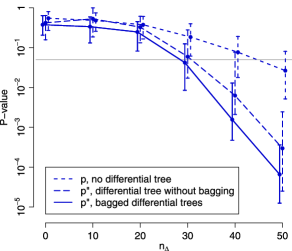
Figure 5: Each vertical line segment represents the central $50\%$ interval of an empirical distribution obtained from $100$ $p$- or $p^{\prime\prime}$-values, and a solid point the median. Some line segments are slightly shifted horizontally for distinguishing purposes. The horizontal line is where $p$-value${}={}$0.05.

Figure 5 shows summaries of the $p$-values ($p$ or $p^{\prime\prime}$) produced by three methods: a direct evaluation using (2) without building any differential tree (which gives the same $p$-value as the root node of a differential tree), building one differential tree, and building differential trees with bagging. The central $50\%$ interval of the empirical distribution of the $p$-value is plotted for each case. It can be seen that, when $n_{\Delta}=0$, all three $p$-values appear to conform well with the uniform distribution on $[0,1]$. We can use the medians of these $p$-values to gauge efficiency and the widths of the central $50\%$ intervals to gauge stability. As $n_{\Delta}$ increases, each $p$-value decreases, and at an increasing rate. The directly evaluated $p$, however, decreases slowly and this approach, on average, is unable to detect the change at the $5\%$ significance level until $n_{\Delta}\approx 44$. An intuitive explanation is that a dramatic change deep under the surface may only manifest as ripples on the surface, that is, at the root node. Also, multiple changes may even cancel out the effects of one another and leave no trace on the surface, as is the case of the differential tree shown in Figure 2. By contrast, with differential trees it “dives” down and seeks differences between the data sets in increasingly smaller areas. The method can thus uncover local differences more efficiently and, for the arson problem, is able to start detecting the change for $n_{\Delta}\approx 31$ (without bagging) and $\approx$27 (with bagging). As $n_{\Delta}$ increases, there are also clearly widening gaps between the $p$-values produced by the direct evaluation method and the differential tree methods. For $n_{\Delta}=50$, the median $p$ is only $2.6\times 10^{-2}$, being barely significant, while the median $p^{\prime\prime}$ is $3.0\times 10^{-4}$ (without bagging) or $6.6\times 10^{-5}$ (with bagging). It is also clear that the bagging technique helped reduce instability and increase efficiency. The arson case has $n_{\Delta}$ close to $60$, which we could not include in the simulation study since it requires $42$ suspicious fires but the most significant pattern has only $41$. However, with a visual extrapolation of the curves in Figure 5 to where $n_{\Delta}=60$, it should be clear that the proposed method is quite effective for discovering the changes in the arson case.

6 Sequential detection

The method developed above can also be used in a sequential detection manner. Let us consider comparing the data of the two consecutive annual periods immediately before a “detection” day (the first day after the two year period). With the quadrennial data available, we start the detection from 1/Jan/2006, by building a differential tree that compares the two time periods, 1/Jan/2004–31/Dec/2004 and 1/Jan/2005–31/Dec/2005, and build new differential trees by shifting the detection day at intervals of seven days, until all data have been examined. From every tree constructed the smallest $p$-value is extracted and adjusted by the Bonferroni and permutation methods, using (10) and (12). The empirical null distribution of the minimum $p$-value in a differential tree that is needed by the permutation adjustment is obtained by permuting $1000$ times the historical fire incidents that occurred during 1/Jan/2004–31/Dec/2005. We have also produced an empirical null distribution by permuting random halves of all the quadrennial data and found that the resulting adjusted $p$-values are only slightly larger, due to the contamination of the irregular changes in the latter two years. The conclusions, however, remain largely the same. To use bagging, one only needs to replace each single differential tree described above with $50$ trees obtained under bootstrap sampling (Section 5.2).

The results are shown in Figure 6. The sequential detection results with bagging shown in Figure 6(b) are clearly more stable than those without bagging in Figure 6(a). From Figure 6(a), after the initial $45$ weeks with basically no significant change discovered and a smallest $p^{\prime\prime}$-value of $0.025$, a sudden decrease of the $p^{\prime\prime}$-value occurred on detection day $316$ (12/Nov/2006) with $p^{\prime\prime}=0.0040$. This is clearly a sign that some significant change(s) have occurred in the underlying data-generating mechanism. Similar conclusions can be drawn from the more stable estimates in Figure 6(b).

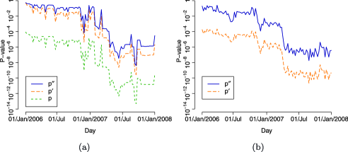
Figure 6: Minimum $p$-values and their adjustments in sequential detection: (a) without bagging; (b) with bagging. In particular, $p$ is the minimum $p$-value in a differential tree, $p^{\prime}$ the Bonferroni adjustment of $p$, and $p^{\prime\prime}$ the permutation adjustment of $p^{\prime}$.

By monitoring the change of (adjusted) $p$-values, it is straightforward for an online system to set up different levels of warning in an easily comprehensible sense.

7 Using different responses

7.1 Using only suspicious fires

Instead of using both suspicious and other fires as done in the study so far, we can use suspicious fires only. Figure 7 displays the differential tree, built analogously to that in Figure 2, from the two biennial subsets. Interestingly, the two most significant patterns are comparable in both trees: one concerning a substantial increase of suspicious fires during almost the same time period and the other a decrease of suspicious fires after it. Note that one cannot use the classification tree approach here, since the response variable has only one level.

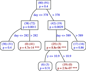
Figure 7: Differential tree built from using suspicious fires only.

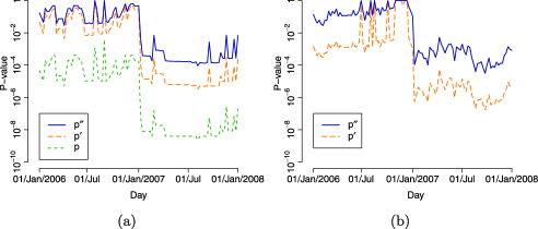
Figure 8: $p$-values in sequential detection using suspicious fires only: (a) without bagging; (b) with bagging.

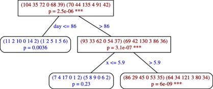
Figure 9: Differential tree built with a different response variable.

The minimum $p$-values and their adjustments for sequential detection are plotted in Figure 8. The sudden change has also been successfully detected, but at a delayed date, as compared with that in Figure 6. This is because most suspicious fires occurred in the latter part of the biennial period (see the histogram of day in Figure 3), and because in the earlier part of the time period there is an increase of fire incidents that are not labeled “suspicious,” which are thus excluded from the study here. In this case, including all fire incidents is preferable—it gives an earlier warning!

7.2 Using an alternative response variable

One can also use a different response variable, as if for a general surveillance, in total ignorance of what has happened. Let us this time treat the variable firetype as the response. The differential tree built from the two biennial subsets is shown in Figure 9. This tree appears to be less informative and its most significant pattern is also less significant, as compared with the trees shown in Figures 2 and 7. However, this discovered pattern is still remarkably significant, showing that the difference is mainly due to an increase of vegetation fires, jumping from $45$ cases to $121$ for day${}>{}$86 and $\mbox{{x}}>5.9$.

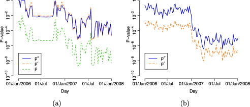
Figure 10: $p$-values in a sequential detection using firetype as response: (a) without bagging; (b) with bagging.

The minimum $p$-values and their adjustments obtained via sequential detection are shown in Figure 10. It is clear that the change has also been detected, at a later date and less dramatically than that in Section 6.

These results are perhaps the most one could hope for when conducting a general surveillance.

8 Concluding remarks

There are two main new ideas in our proposed method for change or difference detection. One is to contrast data sets and model their distributional differences and the other to use tree models to uncover local, irregular changes and provide interpretable results. We followed the general methodology for tree construction. Variants with improved performance likely exist, as in the literature for other families of the tree model. Extensions to other types of difference detection seem fairly straightforward.

Building a differential tree is reasonably fast. With our implementation in R [R Development Core Team (2011)], it took, respectively, $5.0$, $1.4$ and $6.8$ seconds to build the trees shown in Figures 2, 7 and 9, on a workstation with a 2.93 GHz CPU. This made possible the demanding numerical studies reported earlier. If implemented in FORTRAN or C, it is likely much faster.

Finally, we give a rationale for using differential trees in a complex environment. A general alternative is to compare the data with a reference model that can be either exactly known, which is virtually impossible in a complex environment, or estimated from a reference data set, just as we did in Section 4.2. Since building a model from one data set and testing it against the other can waste data information on discovering patterns irrelevant to differences and we are essentially comparing two data sets, why do not we just build one model that directly describes their differences? This is exactly what a differential tree does.

References

- Basseville and Nikiforov (1993) {bbook}[mr] \bauthor\bsnmBasseville, \bfnmMichèle\binitsM. and \bauthor\bsnmNikiforov, \bfnmIgor V.\binitsI. V. (\byear1993). \btitleDetection of Abrupt Changes: Theory and Application. \bpublisherPrentice Hall, \baddressEnglewood Cliffs, NJ. \bidmr=1210954 \bptokimsref \endbibitem
- Breiman (1996a) {barticle}[auto:STB—2012/04/05—08:30:55] \bauthor\bsnmBreiman, \bfnmL.\binitsL. (\byear1996a). \btitleBagging predictors. \bjournalMachine Learning \bvolume24 \bpages123–140. \bptokimsref \endbibitem
- Breiman (1996b) {barticle}[mr] \bauthor\bsnmBreiman, \bfnmLeo\binitsL. (\byear1996b). \btitleHeuristics of instability and stabilization in model selection. \bjournalAnn. Statist. \bvolume24 \bpages2350–2383. \biddoi=10.1214/aos/1032181158, issn=0090-5364, mr=1425957 \bptokimsref \endbibitem
- Breiman (2001) {barticle}[auto:STB—2012/04/05—08:30:55] \bauthor\bsnmBreiman, \bfnmL.\binitsL. (\byear2001). \btitleRandom forests. \bjournalMachine Learning \bvolume45 \bpages5–32. \bptokimsref \endbibitem
- Breiman et al. (1984) {bbook}[mr] \bauthor\bsnmBreiman, \bfnmLeo\binitsL., \bauthor\bsnmFriedman, \bfnmJerome H.\binitsJ. H., \bauthor\bsnmOlshen, \bfnmRichard A.\binitsR. A. and \bauthor\bsnmStone, \bfnmCharles J.\binitsC. J. (\byear1984). \btitleClassification and Regression Trees. \bpublisherWadsworth, \baddressBelmont, CA. \bidmr=0726392 \bptokimsref \endbibitem
- Chaudhuri et al. (1995) {barticle}[mr] \bauthor\bsnmChaudhuri, \bfnmProbal\binitsP., \bauthor\bsnmLo, \bfnmWen Da\binitsW. D., \bauthor\bsnmLoh, \bfnmWei-Yin\binitsW.-Y. and \bauthor\bsnmYang, \bfnmChing Ching\binitsC. C. (\byear1995). \btitleGeneralized regression trees. \bjournalStatist. Sinica \bvolume5 \bpages641–666. \bidissn=1017-0405, mr=1347613 \bptokimsref \endbibitem
- Davis and Anderson (1989) {barticle}[pbm] \bauthor\bsnmDavis, \bfnmR. B.\binitsR. B. and \bauthor\bsnmAnderson, \bfnmJ. R.\binitsJ. R. (\byear1989). \btitleExponential survival trees. \bjournalStat. Med. \bvolume8 \bpages947–961. \bidissn=0277-6715, pmid=2799124 \bptokimsref \endbibitem
- Freund and Schapire (1997) {barticle}[mr] \bauthor\bsnmFreund, \bfnmYoav\binitsY. and \bauthor\bsnmSchapire, \bfnmRobert E.\binitsR. E. (\byear1997). \btitleA decision-theoretic generalization of on-line learning and an application to boosting. \bjournalJ. Comput. System Sci. \bvolume55 \bpages119–139. \biddoi=10.1006/jcss.1997.1504, issn=0022-0000, mr=1473055 \bptokimsref \endbibitem
- Glaz, Naus and Wallenstein (2001) {bbook}[mr] \bauthor\bsnmGlaz, \bfnmJoseph\binitsJ., \bauthor\bsnmNaus, \bfnmJoseph\binitsJ. and \bauthor\bsnmWallenstein, \bfnmSylvan\binitsS. (\byear2001). \btitleScan Statistics. \bpublisherSpringer, \baddressNew York. \bidmr=1869112 \bptnotecheck related\bptokimsref \endbibitem
- Gustafsson (2000) {bbook}[auto:STB—2012/04/05—08:30:55] \bauthor\bsnmGustafsson, \bfnmF.\binitsF. (\byear2000). \btitleAdaptive Filtering and Change Detection. \bpublisherWiley, \baddressChichester, UK. \bptokimsref \endbibitem
- Ishwaran et al. (2008) {barticle}[mr] \bauthor\bsnmIshwaran, \bfnmHemant\binitsH., \bauthor\bsnmKogalur, \bfnmUdaya B.\binitsU. B., \bauthor\bsnmBlackstone, \bfnmEugene H.\binitsE. H. and \bauthor\bsnmLauer, \bfnmMichael S.\binitsM. S. (\byear2008). \btitleRandom survival forests. \bjournalAnn. Appl. Stat. \bvolume2 \bpages841–860. \biddoi=10.1214/08-AOAS169, issn=1932-6157, mr=2516796 \bptokimsref \endbibitem
- Kass (1980) {barticle}[auto:STB—2012/04/05—08:30:55] \bauthor\bsnmKass, \bfnmG. V.\binitsG. V. (\byear1980). \btitleAn exploratory technique for investigating large quantities of categorical data. \bjournalJ. Appl. Stat. \bvolume29 \bpages119–127. \bptokimsref \endbibitem
- Lai (1995) {barticle}[mr] \bauthor\bsnmLai, \bfnmTze Leung\binitsT. L. (\byear1995). \btitleSequential changepoint detection in quality control and dynamical systems. \bjournalJ. Roy. Statist. Soc. Ser. B \bvolume57 \bpages613–658. \bidissn=0035-9246, mr=1354072 \bptnotecheck related\bptokimsref \endbibitem
- MacEachern, Rao and Wu (2007) {barticle}[mr] \bauthor\bsnmMacEachern, \bfnmSteven N.\binitsS. N., \bauthor\bsnmRao, \bfnmYoulan\binitsY. and \bauthor\bsnmWu, \bfnmChunjie\binitsC. (\byear2007). \btitleA robust-likelihood cumulative sum chart. \bjournalJ. Amer. Statist. Assoc. \bvolume102 \bpages1440–1447. \biddoi=10.1198/016214507000001102, issn=0162-1459, mr=2412559 \bptokimsref \endbibitem
- Morgan and Sonquist (1963) {barticle}[auto:STB—2012/04/05—08:30:55] \bauthor\bsnmMorgan, \bfnmJ. N.\binitsJ. N. and \bauthor\bsnmSonquist, \bfnmJ. A.\binitsJ. A. (\byear1963). \btitleProblems in the analysis of survey data, and a proposal. \bjournalJ. Amer. Statist. Assoc. \bvolume58 \bpages415–434. \bptokimsref \endbibitem
- Naus (1965) {barticle}[mr] \bauthor\bsnmNaus, \bfnmJoseph I.\binitsJ. I. (\byear1965). \btitleThe distribution of the size of the maximum cluster of points on a line. \bjournalJ. Amer. Statist. Assoc. \bvolume60 \bpages532–538. \bidissn=0162-1459, mr=0183041 \bptokimsref \endbibitem
- Page (1954) {barticle}[mr] \bauthor\bsnmPage, \bfnmE. S.\binitsE. S. (\byear1954). \btitleContinuous inspection schemes. \bjournalBiometrika \bvolume41 \bpages100–115. \bidissn=0006-3444, mr=0088850 \bptokimsref \endbibitem
- Poor and Hadjiliadis (2009) {bbook}[mr] \bauthor\bsnmPoor, \bfnmH. Vincent\binitsH. V. and \bauthor\bsnmHadjiliadis, \bfnmOlympia\binitsO. (\byear2009). \btitleQuickest Detection. \bpublisherCambridge Univ. Press, \baddressCambridge. \bidmr=2482527 \bptokimsref \endbibitem
- Quinlan (1993) {bbook}[auto:STB—2012/04/05—08:30:55] \bauthor\bsnmQuinlan, \bfnmJ. R.\binitsJ. R. (\byear1993). \btitleC4.5: Programs for Machine Learning. \bpublisherMorgan Kaufmann, \baddressSan Mateo, CA. \bptokimsref \endbibitem
- R Development Core Team (2011) {bmisc}[auto:STB—2012/04/05—08:30:55] \borganizationR Development Core Team (\byear2011). \bhowpublishedR: A Language and Environment for Statistical Computing. R Foundation for Statistical Computing, Vienna, Austria. \bptokimsref \endbibitem
- Shewhart (1931) {bbook}[auto:STB—2012/04/05—08:30:55] \bauthor\bsnmShewhart, \bfnmW. A.\binitsW. A. (\byear1931). \btitleEconomic Control of Manufactured Products. \bpublisherVan Nostrand-Reinhold, \baddressNew York. \bptokimsref \endbibitem
- Su, Wang and Fan (2004) {barticle}[mr] \bauthor\bsnmSu, \bfnmXiaogang\binitsX., \bauthor\bsnmWang, \bfnmMorgan\binitsM. and \bauthor\bsnmFan, \bfnmJuanjuan\binitsJ. (\byear2004). \btitleMaximum likelihood regression trees. \bjournalJ. Comput. Graph. Statist. \bvolume13 \bpages586–598. \biddoi=10.1198/106186004X2165, issn=1061-8600, mr=2087716 \bptokimsref \endbibitem
- Therneau and Atkinson (1997) {bmisc}[auto:STB—2012/04/05—08:30:55] \bauthor\bsnmTherneau, \bfnmT. M.\binitsT. M. and \bauthor\bsnmAtkinson, \bfnmE. J.\binitsE. J. (\byear1997). \bhowpublishedAn introduction to recursive partitioning using the rpart routine. Technical Report 61, Section of Biostatistics, Mayo Clinic, Rochester, NY. \bptokimsref \endbibitem
- Wang et al. (2012) {bmisc}[auto:STB—2012/04/05—08:30:55] \bauthor\bsnmWang, \bfnmY.\binitsY., \bauthor\bsnmZiedins, \bfnmI.\binitsI., \bauthor\bsnmHolmes, \bfnmM.\binitsM. and \bauthor\bsnmChallands, \bfnmN.\binitsN. (\byear2012). \bhowpublishedSupplement to “Tree models for difference and change detection in a complex environment”. DOI:\doiurl10.1214/12-AOAS548SUPPA, DOI:\doiurl10.1214/12-AOAS548SUPPB. \bptokimsref \endbibitem