Short Necklace States, Logarithm Transmission Fluctuation and Localization Length

Abstract

We investigate the widely-existing short necklace states in random systems. It is found that their peak width and relative height in $lnT$ spectra keep almost constant when the system length increases, which is explained by the coupled-resonator theory with intrinsic parameters. This property makes them special in contribution of $lnT$ fluctuation. Further, short necklace states can help us to deeply understand the physical meaning of localization length and the delocalized effect in localized regime.

Anderson localizationAndersonLocalization has changed the basic propagating picture of waves(classical and quantum) in random systems and is used to explain phenomena, e.g. metal-insulator transmission and quantum Hall effects etc. The pioneering studies of quasi one-dimensional (1D) systemsAdditivelnT reveal that the logarithm transmission $lnT$, not the transmission $T$, is statistically Gaussian-distributed and the mean value $\langle lnT\rangle$ over many configurations is linearly additive with the system length $L$. Based on this, the localization length which is the most essential length scale in localization study can be naturally defined as $\xi=-2L/\langle lnT\rangle$. However, unlike $T$ whose fluctuation has been widely studied, surprisingly the $lnT$ fluctuation has not been intensively studied to the best of our knowledge. Obviously, if the origin of the $lnT$ fluctuation is well understood, the physical meaning of localization length can be more deeply revealed.

On the other hand, not all states are localized even in the strongly localized regime, as pointed out in Ref.Pendry1987 ; Tartakovskii that the degenerated localized states can form “necklace states” (NSs) through a 1D random configuration. NSs can generate the mini-bands, i.e. in transmission spectra, which dominate the ensemble average of conductance Pendry1987 ; Pendry1994 . After the NSs are observed in random optical 1D systems Bertolotti2005PRL ; Sebbah2006PRL , some studies have been done, such as the NS probability Bertolotti2006PRE and transmission oscillationGhulinyan2007PRL ; Ghulinyan2007PRA because of different optimal order of NS. Our previous work Chen2011NJP also demonstrates that NSs do not follow the single-parameter-scaling theorem. Recently, Ping Sheng propose that NSs may take a critical role in Anderson phase transition(APT) in his review on ScienceShengPingPercolation . Such proposing shows that many details of APT are still not well understood and the relation between APT and NSs needs more study. But numerically and experimentally, for $L\gg\xi$ configurations, it is found that NSs are so extremely rare that it is hard to find one even in millions of configurations. Then it is rational to doubt whether NSs are qualified to take the critical role in APT or important for localization study. If some kinds of NS widely exist in almost all random configurations and almost all frequency ranges, then the role of NS could be changed radically.

After careful review, we find that previous NS studies are focused on long necklace state(LNS) which is spatially extended through a whole configuration. The length is an important property of NS, but it is secondary. The most essential property of NS is the coupling between localized states which are near to each other in both frequency domain (nearly degenerated) and in spatial domain so that they form a “chain”(necklace) and help wave to hop from one to another. If we disregard the length requirement, e.g., a few localized states form a chain which is so short that it is deeply embedded inside a long configuration, we define such a chain as short necklace state(SNS). Obviously, the occurrence probability of SNS is much much higher than LNS. Then the question becomes “Are there special properties of SNSs which make them very important in localization studies?”

In this Letter, we will demonstrate that the high plateau in $lnT$ spectra are the evidence of widely existing SNSs. SNSs are an important origin of the $lnT$ fluctuation and very essential for fully understanding the physical meaning of localization length. The most special property of SNSs is that their peak width and the relative hight in $lnT$ spectra depend only on intrinsic parameters, i.e. the coupling strength between localized states and the length of SNS, and is independent of configuration length $L$. This property is found numerically and also derived by our theory based on the coupling-resonator model. So SNSs have priorities over LNSs since their much higher occurrence probability, and also have priorities over localized states since their much wider and almost $L$-independent peak-width. Further more, we demonstrate that the localization length $\xi$ is not a simple ‘decay length’ since it includes the delocalized effects of SNSs. With all these results, a basic physical picture can be formed in which SNSs are the widely existing seeds of delocalization effect even in the strong localized regime and can help us to understand details of APT.

Our numerical 1D model is made of optical binary layers, i.e. each cell contains two kind layers, whose dielectric constants are $\epsilon_{1}=1$ and $\epsilon_{2}=2$, and thicknesses are $d_{1}=95nm$ and $d_{2}=d_{2}^{0}(1+W\gamma)$ where the randomness is introduced, $d_{2}^{0}=120nm$ is the average thickness, $\gamma$ is the random number in the range of $[-1,1]$ and $W$ is the randomness strength which is chosen as 0.1 in this work.

Following the history of localization study, we start from the statistic property of $lnT$ of configurations. The $lnT$ distribution of $2\times 10^{5}$ configurations for 3000-cell and 6000-cell systems at frequency $f_{0}=2.5422\times 10^{15}$Hz are shown in Fig.1. Same as expected, $lnT$ is Gaussian distributed. From the $\langle lnT\rangle$, we can obtain $\xi=-L/\langle lnT\rangle=150a_{0}$, where $a_{0}=d_{1}+d_{2}^{0}$ is the average cell length and chosen as the length unit. The Gaussian distribution of $lnT$ is well known, but the physical reasons of $lnT$ fluctuation, which related with basic understanding of localization length, is still waiting for more detailed study.

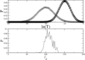
Figure 1: Fig.1a, the $lnT$ distribution of 3000-cell and 6000-cell configurations. Fig.2b, the distribution of decay length $l_{d}$ of localized states in $L=10\xi$ configurations.

The first naive thought of the $lnT$ fluctuation is that it’s originated from the resonant transmission peaks of localized states, such as Azbel statesAzbel . But from simple scaling argument, we will find out these peaks are negligible in $lnT$ fluctuation for enough long systems, $e.g.$, $L>10\xi$. The contribution of localized state peaks can be roughly estimated as $P*H$, where $P$ is the probability of a frequency exactly falling on a resonant peak, and $H\sim L/\xi$ is the averaged hight of peaks in $lnT$ spectra. $P$ is $\propto\rho{\delta\omega}$, where $\rho\propto L$ is the density of state and ${\delta\omega}$ is the peak average width of localized states. Since peakwidth $\delta\omega\propto e^{-L/\xi}$ decrease exponentially with L, the contribution to $lnT$ fluctuation from localized state peaks can be neglected when $L\gg\xi$.

The second naive thought is that the $lnT$ fluctuation is from the different decay length $l_{d}$ of the localized states. But after numerical calculation of $l_{d}$ from field distribution of localized states in $3\times 10^{4}$ random configurations with $L=10\xi$, we find that the distribution of $l_{d}$, shown in Fig. 1b, is quite different from that of $lnT$. We can see that the distribution of $l_{d}$ is not Gaussian and its mean value is about $l_{d}\sim 100$ much smaller than $\xi=150$. The difference between $l_{d}$ and $\xi$ will be discussed later.

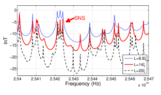
Figure 2: The spectra of three configurations. The longer one is constructed by adding layers to shorter ones.

To find the physical reason of the fluctuation of $lnT$, we need to check the $lnT$ spectra of random configurations for details. Three typical $lnT$ spectra are shown in Fig.2 of random configurations with length $8.8\xi$, $L=14\xi$ and $L=20\xi$. The longer configuration in Fig.2 is constructed by adding more layers to the shorter configuration(keeping the original part unchanged). At first sought, the spectra are like the “fish backbone” with the sharp resonant peaks of localized states as “stings”. But we note that the base of backbone is not quite flat and there are plateaus and valleys which are higher or lower than the mean value $\langle lnT\rangle=-L/\xi$. These plateaus and valleys are the basic spectral feature of one certain configuration. For totally different configurations, the feature (the positions of plateaus and valleys) are totally different. Hence, it is rational to think that the fluctuation of $lnT$ at certain frequency is mainly from these plateaus and valleys of different configurations. Actually, not only fluctuation of $lnT$, the mean value $\langle lnT\rangle$, which defined the localization length $\xi$, is also averaged over all valleys and plateaus for different configurations at certain frequency. Then the question becomes “where are these plateaus and valleys from?”.

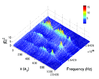
Figure 3: The field intensity $|E|^{2}$ versus $x$ and $f$ of the necklace state signed in Fig.2

After careful observation, we find that, although the plateaus and valleys are quite different for totally different configurations, the spectral feature has some kind of inheritance, if we increase the system length $L$ by adding more layers at both sides of the original configuration, as we did in Fig.2. The inheritance of the spectra is clearly shown in Fig.2, where the longer configuration is constructed by adding more layers to the shorter one. The inheritance infer that these plateaus and valleys are not sensitive to the boundary of a configuration, or in other words, they are really from intrinsic things deeply inside a configuration. After careful check, we find that the origin of the plateaus in transmission spectra is the SNS which widely exist deeply inside long configurations. From Fig.2, we can clearly see that, for short configuration with $L=8.8\xi$, there is a LNS signed by red arrow which is same as that predicted by Pendry and Tartakovskii Pendry1987 ; Tartakovskii . The field distribution at resonant frequencies shown in Fig.3 also confirm the judgement. After adding more layers, for $L=24$ configuration, the plateau is still there, but much lower and now the LNS becomes SNS which deeply embedded inside the longer configuration. Inversely, if we find a SNS plateau in the spectra of a long configuration, we can locate the position of SNS by the field distribution at the resonant frequencies, then, by removing more layers far away from the SNS, we change the SNS into LNS of a shortened configuration. So, SNS and LNS could be transformed into each other by adding or removing more layers. But for very long configurations, compared with extremely rare LNS, SNS widely exist in almost all frequency range.

With SNS concept in random configurations, we can understand the $lnT$ spectra of random configurations in a very different picture now. Without SNS, the spectra of random configurations are formed by randomly distributed peaks of independent localized states, so that the fluctuation is only from fluctuation of density of states. But now, we know that the coupling between a few localized states can generate correlation in $lnT$ spectra, which is represented by many small plateaus. Actually, compared with LNS which generate correlation in $T$ spectra which have been studied by Pendry and our previous work Chen2011NJP , SNS can generate correlation in $lnT$ spectra chenjiang . Widely existing SNS plateaus form the basic feature of $lnT$ spectra, as shown in Fig.2. But SNS population is still much less than localized states. Next, we will show that an important property of SNSs makes them much more important than localized states as the source of $lnT$ fluctuation.

Comparing the signed plateaus in Fig.2 with different $L$, we find that their width and relative hight keep almost constant, although the absolute hight is reduced with $L$. This property makes SNS qualitatively different. The contribution of localized states to the $lnT$ fluctuation can be neglected for long systems ($L\gg\xi$) since their peak-width decreases exponentially with length, while the SNS contribution of $lnT$ spectra is much larger since their constant peak width and relative hight.

Why the width and hight of SNS are almost constant for different $L$? And, with increasing length L by adding more layers, why most plateaus are robust but some of them will split? We will reveal the physics behind these SNS properties. From different behaviors of plateaus, we can separate the SNS plateaus into two classes, the short intrinsic NS (SINS) for the robust ones and short non-intrinsic NS (SNNS) for the splitting ones. We use the coupled-resonator model to study the difference between two classes. Suppose that two localized states, whose frequencies and positions are near to each other, can be represented by two coupled resonators:

$$\ddot{E_{1}}+\delta_{1}\dot{E_{1}}+\omega_{1}^{2}E_{1}=\kappa_{12}\dot{E_{2}}$$

$$\ddot{E_{2}}+\delta_{2}\dot{E_{2}}+\omega_{2}^{2}E_{2}=\kappa_{21}\dot{E_{1}}$$ (1)

where $E_{i}$, $i=1$ or $2$, are the fields of two localized state, and $\dot{}$ means the time derivative; $\omega_{i}$ and $\delta_{i}$ are the “original” central frequencies and peak-widths (inverse of quality factors) of two localized states if without coupling, and $\kappa_{12}=-\kappa_{21}\propto\int dx(E_{1}*E_{2})$ are the coupling strength between two localized states which proportional to the overlap integral. To classify these different behaviors, we need to compare scales of several parameters in Eq.(1). First, supposing that the sum of original peak-widths $\delta_{1}+\delta_{2}$ is larger than peak distance $\Delta\omega_{12}=|\omega_{1}-\omega_{2}|$ which means two peaks overlapping with each other. For example, a configuration length $L$ is not very long so that two peaks are wide enough to overlap with each other, then, two peaks form a plateau. But, when the length $L$ increases by adding more layers, both peak widths $\delta_{i}$ decrease exponentially, then, when $\delta_{1}+\delta_{2}<\Delta\omega_{12}$, whether the plateau will split or not depends on a new condition, the comparing between $|\kappa_{12}|$ and $|\Delta\omega_{12}|$. From the coupled-resonators theory Landau , we can obtain that, if the condition

$$\kappa_{ij}>\Delta\omega=\omega_{i}-\omega_{j}$$ (2)

is satisfied, two resonators are always well-coupled to each other and now the plateau width is determined by $\kappa_{ij}$(peak-repulsion effect), independent of any other conditions . If this condition is not satisfied, the plateau will split when $L$ is large enough. For multi-coupled localized states of $n$th-order SNS, the discussion is similar. Now, the reason of different behaviors of plateaus is obvious, for the SINS, the plateau is very robust and its width is determined by coupling strength, but for SNNS, the plateau will split. For long $L>>\xi$ configurations, most plateaus are from the SINS which are deeply embedded inside the configurations, while very few exceptions are generally near the configuration edges since the peak width of near-edge localized states is much larger. In following discussion of this work, all SNS are referred to SINS. From Eq.(2), we can also obtain the optimal distance of localized states in SNS optd .

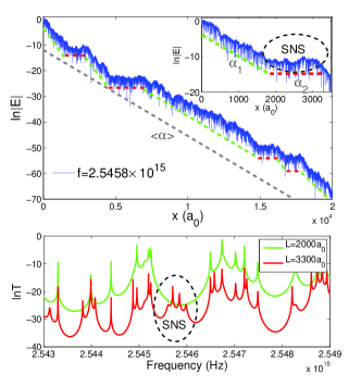
Figure 4: Fig4a, the $ln|E(x)|$ vs $x$ of a configuration with $2\times 10^{4}$ cells, and the “slope sections” are singed by dashed lines. The insert is the enlarged part of first $3000$ cells. Fig4b, the $lnT$ spectra of two configurations with first $2000$ cells (first slope section) and $3300$ cells(including first and second slope section) of Fig.4a configuration.

Next, we will demonstrate that the localization length $\xi=-L/\langle lnT\rangle$, the most important length scale in Anderson localization theory, is related with SNS too. It’s well known that there is a “save” way to obtain the precise $\xi$ numerically, .i.e. calculating the electric field $E(x)$ of a $very$ $long$ random configuration at a chosen frequency, then $\xi$ can be obtain as the inverse of slope $\xi\simeq-L/ln(E(L)/E(0))$. The violation will be very small for very large $L$, since the variance $\sigma\propto\sqrt{L/\xi}$ is much smaller than mean value $-L/\xi$, which is called as self-averaging property. However, if we are careful, more interesting details can be found as shown in Fig. 4a, where $ln|E|$ vs $x$ at frequency $f=1.5996\times 10^{16}$Hz is shown. The insert is the enlarged first small part of Fig.4a for detailed discussion. We find that, except short-range fluctuations, there are several long-range “sections” signed by dashed lines as shown in Fig.4a. In each section, the slope $\alpha_{i}$ does not have large change, but in different sections the slopes could be quite different, which is clearly shown in $\alpha_{1}$ and $\alpha_{2}$ in Fig.4a insert. Where are these ”sections” from? We can find the reason if we check two $lnT$ spectra shown in Fig.4b, which are from two configurations with the $2000$ cells and the first $3300$ cells of the long configuration in Fig.4a. The first configuration ($I_{conf}$) exactly includes first section of Fig.4a insert, while the second configuration ($II_{conf}$) includes both first and second sections. For $I_{conf}$ whose slope in Fig.4a is very larger(compared the average slope), we find that the frequency is exactly falling into the spectrum valley. But for $II_{conf}$ which ends with very-small-slope section, we find that there is a SNS appearing at the frequency, and again the inheritance is very clear for two spectra. Obviously, the occurrence of SNS has strong influence on the local slope and determined a “very-small-slope section”. Another important influence of slope is from fluctuation of density of states(very few states in the valley), but it is not the main topic of this work. With these observation, we can construct such a more detailed picture to describe the decay slope of $ln|E|$ when configuration length $L$ increases: if a SNS occurs, the slope will be much smaller, but if without SNS and even very few localized states occurs, the slope will be much larger. Based on SNS picture, three conclusions are derived from observation. The first is that the typical “section” length (about $10\xi$ in our model) actually is the typical length scale $l_{NS}$ for a SNS to appear at certain frequency. Second, we have new understanding of the localization length $\xi$, since, for a very long configuration, many short SNS in it have strong influence not only on the slope of sections, but also on the total average slope $\overline{\alpha}$, which is the inverse of $\xi$. Third, we have new understanding of self-averaging property of $lnT$ spectra too, i.e. the average slope of a very long system has not only averaged the density fluctuation of localized states, but also averaged the occurrence fluctuation of SNS. Our recent work Chen2011NJP shows that the occurrence probability $P_{NS}$ of LNS will increases considerably near APT point, so that NS is not confined by single parameter theorem and could take a critical delocalization role at APT. In this work, we can see that, even in very strong localized regime, SNS represent widely existing delocalization mechanism. SNS may can tell us more details of the APT scenario, i.g. more and more SNS can be connected with each other and form a LNS at last, so that the whole configuration is conducting.

At last, we hope to discuss the decay length $l_{d}$ of localized states and its relation with $\xi$. As we have shown in Fig.1b, the $l_{d}$ typical value of configurations with $L=10\xi$ is very different from $\xi$, which is against our common sense since we generally use $exp(-L/\xi)$ to represent the field of localized states. Numerical results tell us that, for not-very-long $L<2l_{NS}=20\xi$ configurations, $l_{d}$ typical value is smaller than $\xi$. Our explanation is following: since there is no SNS in such not-very-long system generally, $l_{d}$ is the “naked” decay length which is corresponding the large slope in Fig.4a, and the field should be write as $exp(-L/l_{d})$. Only in the very long range ($x>>l_{NS}$), the localized field can approximated as $exp(-|x|/\xi)$ since all effects of SNS are included.

In summary, the SNSs which widely exist in long random configurations are investigated. The speciality of SNSs and their contribution to $lnT$ fluctuation and localization length $\xi$ are studied numerically and theoretically. With SNSs, a much more detailed picture of Anderson phase transition can be set up, and many topics can be quantitatively studied, such as the evolution of SNS with strength of randomness, the change of localization length and its relation with evolution of SNS, the correlation in $lnT$ spectra and the optimal order of SNS. These studies will reveal more details of APT in future.

References

- (1) P. W. Anderson, Phys. Rev. 109, 1492 (1958); P. A. Lee, T. V. Ramakrishnan, Rev. Mod. Phys. 57, 287 - 337 (1985); Photonic Crystals and Light Localization in the 21st Century, edited by C. M. Soukoulis (Kluwer, Dordrecht, 2001); P. Sheng, Introduction to Wave Scattering, Localization, and Mesoscopic Phenomena, Second Edition (Springer, Berlin 2006).
- (2) E. Abrahams, P. W. Anderson, D. C. Licciardello and T. V. Ramakrishnan, Phys. Rev. Lett. 42, 673 (1979); P. W. Anderson, D. J. Thouless, E. Abrahams, D. S. Fisher, Phys. Rev. B 22 3519 (1980);
- (3) J. B. Pendry, J. Phys. C 20 733 (1987).
- (4) A. V. Tartakovskii et al., Sov. Phys. Semicond. 21, 370 (1987).
- (5) J. B. Pendry, Adv. Phys. 43 461 (1994).
- (6) J. Bertolotti, S. Gottardo, D. S. Wiersma, M. Ghulinyan, L. Pavesi, Phys. Rev. Lett. 94 113903 (2005).
- (7) P. Sebbah, B. Hu, J. M. Klosner, and A. Z. Genack, Phys. Rev. Lett. 96 183902 (2006).
- (8) J. Bertolotti, M. Galli, R. Sapienza, M. Ghulinyan, S. Gottardo, L. C. Andreani, L. Pavesi, D. S. Wiersma, Phys. Rev. E 74 035602 (2006).
- (9) M. Ghulinyan, Phys. Rev. Lett. 99, 063905 (2007).
- (10) M. Ghulinyan, Phys. Rev. A 76, 013822 (2007).
- (11) P. Sheng, Science, 313 139-140 (2006).
- (12) L. Chen, W. Li, X. Jiang, New J. Phys. 13 053046 (2011).
- (13) M. Ya. Azbel, Paul Soven, Phys. Rev. B 27, 831 (1983); M. Ya. Azbel, D. P. DiVincenzo, Phys. Rev. B 30, 6877 (1984).
- (14) The studies of correlations will be published elsewhere.
- (15) L. D. Landau and E. M. Lifshitz, Mechanics, Course of Theoretical Physics Vol. 1, 3rd ed. (Pergamon, Oxford, 1976).
- (16) We can evaluate the “optimal distance” of localizes states in SNS by the , where is the probability for a localized state to find another nearly-degenrated localized state in distance . Since and where is the decay length of localized field, we can obtain the optmal distance as , which agree with our numerical observation very well.