Stochastic Resonance in Periodic Potentials Revisited.

Abstract

The phenomenon of Stochastic Resonance (SR) has been conclusively demonstrated in bistable potentials. However, SR in sinusoidal potentials have only recently been shown numerically to occur in terms of hysteresis loop area. We show that the occurrence of SR is not specific to sinusoidal potentials and can occur in periodic bistable potential, $U(x)=\frac{2}{3}(\cos x+\cos 2x)$, as well. We further show that SR can occur even in a washboard potential, where hysteresis loops normally do not close because of average drift of particles. Upon correcting for the drift term, the closed hysteresis loop area (input energy loss) shows the usual SR peaking behaviour as also the signal-to-noise ratio in a limited domain in the high drive-frequency range. The occurrence of SR is attributed to the existence of effectively two dynamical states in the driven periodic sinusoidal and periodic bistable potentials. The same explanation holds also when the periodic potentials are tilted by a small constant slope.

I Introduction

The phenomenon of stochastic resonance (SR), initially put forth theoretically to explain the occurrence of ice ages, at a certain frequency, on earthBenzi , have been observed experimentally in many physicalFauve ; Roy and biological systemsDouglass ; Moss . SR has been investigated theoretically and experimentally with considerable interest over the past three decadesGamma ; Well . Its attraction lies in the seemingly counter-intuitive idea that by tuning noise level (externally or internally) the response of a nonlinear system to a weak external periodic signal can be enhanced considerably; or a nonlinear system itself tunes the noise level in order to enhance a particular chosen signal. Moreover, the noise level at which the response peaks depends on the frequency of the input signal. As a consequence, it may have potential applications in the detection of weak signals as well as in the selection of a signal of a particular frequency out of a host of signals of different frequenciesMantegna ; Murali ; Mohanty ; Collins . As a corollary, a biological system can tune noise level internally to select and enhance a desired signalGluckman ; Simonotto ; Taba . Apart from potential practical applications, it offers considerable theoretical challenges. The occurrence of SR in bistable systemsGamma ; McN has more or less been confirmed and reported fairly widelyGamma ; Well . However, its occurrence in periodic potentials is still debatableKim , though there have been some investigations in monostableStocks and periodic potential systemsDykman as well.

There have been some discussion on SR in periodic potentials in view of obvious practical importance of these potentials, such as in describing motion of adatoms on crystal surfacesGraham , superionic conductivity, RCSJ model of Josephson junctionKauf ; Barone ; Risken , etc. The conventional SR is considered to occur in a bistable system at a temperature when the signal frequency matches the time rate of passage across the potential barrier of the nonlinear systemKim ; McN . Analogously, one would expect, for instance, the frequency dependent mobility, as a response, to peak as a function of temperature, at a signal frequency corresponding to the mean passage rate across a potential barrier of the periodic potential. However, instead, the mobility shows monotonic behaviour around that frequency. It does show a peak with temperature only at a much higher frequency. This mobility peaking with temperature is termed as a kind of dynamical resonance, unlike the SR satisfying the conventional criterion of frequency matching, and merely confined to intrawell motionKim ; Stocks ; Dykman . This aspect has been examined more closely in a recent numerical workPRE on a sinusoidal potential considering hysteresis loop area as response to the input signal $F(t)=\Delta F\cos\omega t$.

Hysteresis loop area (HLA), in the average position-forcing, $(x-F)$, space, or equivalently, the input energy lost by the system to the environment per period of the external forcing $F(t)$, is considered as an appropriate measure of SR. HLA has been considered as a quantifier of SR earlier tooSRS ; Iwa . However, recently HLA was found to show SR behaviour close to what was shown by the amplitude of the average particle-position variable $x(t)$ in a bistable systemHein ; Saikia ; Sahoo ; Jop . HLA not only includes information of the mean amplitude $x_{0}$ of $x(t)$ but also its phase relationship with the external forcing or the input signal $F(t)$. Its significance as an appropriate quantifier of SR has also been pointed out recentlyEvstigneev ; Jung . Moreover, in a periodic potential, it is very likely that the particle forays into wells far away, on either direction, from the initial well. It makes the position variable unsuitable for any meaningful quantification of SR. It is found that the HLA or input energy loss takes account of motion whether it is in a single well or spread over several wells. Also, HLA shows qualitatively similar behaviour as the frequency dependent mobility calculated using the linear response theoryKim . The HLA has recently been used as a quantifier of SR in a underdamped periodic potential systemPRE .

In Ref.PRE it was pointed out that the peaking of HLA as a function of temperature at high frequencies ought not to be dismissed as merely a dynamical resonanceKim . The phenomenon can be seen as a result of transitions between two dynamical states of the damped driven particle trajectories in the highly nonlinear (sinusoidal) potential. The two and only two dynamical states exist and are distinguished by their trajectory amplitudes and their phase relationship with the field $F(t)$. The relative stability of the two states changes as the temperature (noise strength) is varied.

It is hard to prove analytically that an underdamped particle moving in a sinusoidal potential driven by a periodic force of frequency close to the natural frequency at the bottom of a well of the potential and subjected to fluctuating forces can have only two dynamical states of its trajectories as it was found numerically. Solution of only the simplest situation of the deterministic motion of a driven pendulum without friction,
$m\frac{d^{2}x}{dt^{2}}=-\frac{\partial}{\partial x}(-\sin x)+F_{0}\cos\omega t$,
given the initial condition $(x(0),v(0))$, can be obtained analytically and its phase trajectories drawnLaksh . Notice that the periodic potentials $U_{0}(x)=-\sin x$ and $U_{0}(x)=\cos x$ are equivalent except for a phase difference of $\pm\frac{\pi}{2}$. Also, the trajectories with initial conditions $(x(0),0)$ and $(2\pi-x(0),0)$ should be identical except that they are in opposite directions in case of closed orbits and in $\pm v$ sectors in case of travelling solutions. In other words, the two trajectories should have the same amplitude but different phase relationship with the external forcing. However, for different initial conditions ($x(0),v(0)$), they can have different trajectories and not necessarily confined to just two particular trajectories. But, when damping is present, it is easy to appreciate that if two trajectories have different phases they will necessarily have different amplitudes and hence different energy contents. This can be seen as follows.

Figure 1: The figure shows the periodic potential when $F(t)=0$ (curve $O$), $F(t)=\Delta F$ (curve $A$) and $F(t)=-\Delta F$ (curve $B$).

Consider the two extreme cases of particle motion being (i) in-phase, and (ii) completely out-of-phase with the external drive. Fig. 1 shows the periodic potential when $F(t)=0$ (curve O), $F(t)=\Delta F$ (curve A), and $F(t)=-\Delta F$ (curve B), where $F(t)=\Delta F\cos\omega t$, so that the total potential $V(x)=-\sin x-x\Delta F\cos\omega t$. Consider the extreme position P1 of the particle on the curve A when $F(t)=\Delta F$. In the next moment the $F(t)$ will decrease and also the particle position moves to the left so that $F(t)$ and $x(t)$ are in phase. They being in phase implies that when $F(t)=0$ the particle is at the potential bottom P2 and when $F(t)=-\Delta F$ the particle is at P3, the extreme position on the left and is about to roll down the potential hill as $F(t)$ begins to rise from $-\Delta F$. From the figure, therefore, one could notice that in this case of in-phase situation the particle always moves on the stiffer slope of the potential $V(x)$. On the other hand, if we were to begin from the particle position P4 on A while $F(t)=\Delta F$, the particle always moves lying on the gentler slope of $V(x)$ in this completely out-of-phase case. Since the force experienced by the particle due to the potential in the two cases have different values one would naturally expect the damped particle to have different amplitudes of motion and hence have different energy losses due to frictional forces. The two dynamical states are thus distinct.

At low temperatures, for given $F(t)$, depending only on the initial conditions the system chooses one of the two dynamical states. These two states are quite stablePRE and no transition occurs between them. However, as the temperature is increased transition takes place between the dynamical states and, as a result, the relative population of these states changes. Thus, the mean amplitude of the trajectories and the overall phase when averaged over the initial conditions vary with temperature. The hysteresis loop area shows a peak at a temperature indicating stochastic resonance where the transition rate between the dynamical states acquires a particular value. It is also important to notice that well before the HLA peaks, the particle begins to surmount the potential barrier of $V(x)$ and at resonance the motion is no longer confined to a single well of $V(x)$; the inter-well transitions become quite numerous. Of course, the inter-well transition rate is still quite low compared to the transition rate between the dynamical statesPRE .

In the present work, we show that a driven underdamped particle exhibits stochastic resonance in (i) a periodic bistable potential, $U(x)=\frac{2}{3}(\cos x+\cos 2x)$, and also in (ii) washboard potentials (tilted sinusoidal as well as tilted periodic bistable potential). In this work we use HLA as a quantifier of SR but also supported by the signal-to-noise ratio (SNR).

The appropriateness of the HLA as a quantifier of SR vis-a-vis the SNR has been discussed extensively in Ref.Evstigneev . However, the SNR has been used in many earlier works to discuss SR. Without going into the relative merits of these quantifiers we present the SNR to complement extensive results that we show in terms of HLA. As has been pointed outEvstigneev the quantifiers do not peak at the same temperature. However, our main contention that SR is a distinct possibility in periodic potentials is reinforced by the results of SNR.

Figure 2: The periodic bistable potential $U(x)=\frac{2}{3}(\cos x+\cos 2x)$ is shown with two similar subwells in a well of the potential.

In the case of bistable periodic potential too, effectively, two and only two dynamical states (one in-phase and one out-of-phase) of trajectories of a periodically driven underdamped particle are obtained. Since in a potential well of $U(x)$ there exist two similar subwells (Fig. 2) there are two (one in-phase and one out-of-phase) states in each subwell. The in-phase (out-of-phase) state in one subwell has the same amplitude and phase relationship as the in-phase (out-of-phase) state in the other subwell. Therefore, energetically there exist only one in-phase and one out-of-phase states of trajectories. However, as time progresses, these trajectories can also be in wells and subwells other than the initial ones, the basins of attraction of the dynamical states can be identified in different wells and subwells. Consequently, the basins of attraction of the dynamical states become more complex than in case of sinusoidal potentials where only trajectories in different wells are distinguished.

In the case of periodic bistable potentials HLA, as also the signal-to-noise ratio, shows a peaking behaviour, just as in the case of sinusoidal potential, as the temperature is varied. The non-monotonic behaviour of HLA as a function of temperature is related to the relative stability of the in-phase and out-of-phase states of trajectories. Moreover, the particle does make inter-well transitions also.

The washboard potentials, that is a slanted sinusoidal potential and slanted bistable periodic potential, naturally yield finite particle drifts. As a consequence the hysteresis loops do not close. However, upon correcting for the drift factor, as explained in Sec. III, the hysteresis loops close and the closed hysteresis loop areas could be made to agree with the input energy loss. The HLA (or the input energy loss) so obtained again shows peaking behaviour as the temperature is varied. This is a clear signature of SR in the washboard potential. The occurrence of SR could again be explained in terms of transition between the two dynamical (one in-phase and one out-of-phase) states of particle trajectories that are realized even in these washboard potentials.

II The model

We consider motion of an underdamped particle along (i) a periodic bistable potential $U(x)=\frac{2}{3}V_{0}(\cos x+\cos 2x)$, (ii) a tilted sinusoidal potential $U_{1}(x)=-V_{0}\sin kx-F_{0}x$, and (iii) a tilted bistable potential $U_{2}(x)=U(x)-F_{0}x$, where the tilt $F_{0}$ represents a constant force. As mentioned earlier (Fig.2) $U(x)$ has two subwells of equal depth (bistable) in each periodic well of the potential. $U(x)$ is symmetric about $x=n\pi$, where, $n=\mp 1,\mp 2,\cdots$. The latter two potentials we shall refer to as the washboard potential and the bistable washboard potential, respectively, for $F_{0}\neq 0$ but small. In the bistable washboard potential $U_{2}(x)$ the two subwells exist but are no longer identical as they were in $U(x)$.

A particle of mass $m$ moving in a medium of friction coefficient $\gamma$ along a potential $V(x)$ and driven by an external periodic forcing $F(t)=\Delta F\cos\omega t$ and subjected to a Gaussian white noise $\xi(t)$, is described here by the Langevin equation,

$$m\frac{d^{2}x}{dt^{2}}=-\gamma\frac{dx}{dt}-\frac{\partial{V(x)}}{\partial x}+F(t)+\sqrt{\gamma T}\xi(t).$$ (1)

The fluctuating forces $\xi(t)$ satisfy: $<\xi(t)>=0$ and $<\xi(t)\xi(t^{{}^{\prime}})>=2\delta(t-t^{{}^{\prime}})$. The temperature $T$ is in units of the Boltzmann constant $k_{B}$. We take $V(x)=U(x),U_{1}(x)$, or $U_{2}(x)$ separately to discuss the nature of particle motion.

The equation is written in dimensionless units by setting $m=1$, $V_{0}=1$, $k=1$. The Langevin equation, with reduced variables denoted again now by the same symbols, corresponding to Eq. (2.1) is written as

$$\frac{d^{2}x}{dt^{2}}=-\gamma\frac{dx}{dt}+cosx+F(t)+\sqrt{\gamma T}\xi(t).$$ (2)

The noise variable, in the same symbol $\xi$, satisfies exactly similar statistics as earlier.

III Numerical Results

We adopt the same numerical procedures as described in Ref.PRE . The drive (signal) frequency ($\omega=\frac{2\pi}{\tau}$) is chosen to be close to but a little smaller than the natural frquency at the bottom of the wells of the potentials. However, they are not exactly equal to the respective natural frequencies (without damping). For the periodic bistable potential $U(x)$, we take the period $\tau$ equal to 4.8. The same optimum $\tau$ is taken also for the bistable washboard potential $U_{2}(x)$. Similarly, we continue with $\tau=8$ as in Ref.PRE for the washboard potential $U_{1}(x)$.

With the periods $\tau$ of the external forcing $F(t)=\Delta F\cos\omega t$, we obtain the trajectories $x(t)$ for given initial conditions $(x(0),v(0))$ numericallyNume ; SRS by solving the Langevin equation (2.2) and calculate the input energy, or work done by the field on the system, $W$, in a period $\tau$, asSeki :

$$W(t_{0},t_{0}+\tau)=\int_{t_{0}}^{t_{0}+\tau}\frac{\partial U_{e}(x(t),t)}{\partial t}dt,$$ (3)

where, the effective potential $U_{e}(x(t),t)=V(x)-xF(t)$, and $V(x)=U(x),U_{1}(x)$, or $U_{2}(x)$ as applicable. Therefore,

$$W(t_{0},t_{0}+\tau)=-\int_{F(t_{0})}^{F(t_{0}+\tau)}xdF=A,$$ (4)

where $A$ is the magnitude of the HLA. The average input energy per period, $\overline{W}$, averaged over an entire trajectory spanning $N_{1}$ periods of $F(t)$, is

$$\overline{W}=\frac{1}{N_{1}}\sum_{n=0}^{n=N_{1}}W(n\tau,(n+1)\tau)=\overline{A}.$$ (5)

Typically, $N_{1}$, ranges between $10^{5}$ to $10^{7}$, as required.

At very low temperatures $\overline{W}$ depends very strongly on the initial conditions ($x(0),v(0)$). This is because whether the trajectories are in the in-phase state (with a small phase difference $\phi_{1}$ between $x(t)$ and $F(t)$) or in the out-of-phase state (with a large phase difference $\phi_{2}$) is determined by the initial condition. And, $\overline{W}$ depends on the kind of trajectory. Moreover, at such temperatures the particle remains trapped in the initial well of the potential and also no transition between in-phase and out-of-phase states of trajectories takes place in a well. However, as the temperature is gradually increased the intra-well transitions between the in-phase and out-of-phase states begin to take place and subsequently, inter-well transitions also become frequent. Therefore, as the temperature is increased the dependence of $\overline{W}$ on the initial conditions ($x(0),v(0)$) weakens. However, it is always sensible to ensemble average $\overline{W}$ over all possible initial conditions and obtain the average input energy per period $<\overline{W}>$, which is also equal to the mean hysteresis loop area $<\overline{A}>$, Eq. (3.3).

As mentioned earlier, the response $x(t)$ in the two dynamical phases of trajectories not only have different phase relationship with the forcing $F(t)$ but the mean amplitude $x_{0}$ of $x(t)$ in the two cases are very different. Therefore, apart from the inherent stochastic nature of $W$ ( Eq. 3.1) the values of $W$ are different depending on whether, during the particular period (of $F(t)$) in question, the system is in the in-phase or in the out-of-phase state of trajectory or makes transition(s) between the states. A clear picture is revealed by the distribution $P(W)$ of input energies at various temperatures. For sinusoidal potentials the evolution of $P(W)$ with temperature furnishes important information on the occurrence of SRSaikia ; Sahoo ; Jop . Also, since the entire stretch of the trajectories consists of a mixture of in-phase (with phase $\phi_{1}$) and out-of-phase (with phase $\phi_{2}$) states, the average phase lag $\phi$ must lie between $\phi_{1}$ and $\phi_{2}$. Naturally, $\phi$ is a function of temperatureLGamma ; Dykman1 . The phase $\phi$ is obtained numericallyPRE by calculating the mean hysteresis loops $<\overline{x}(F(t_{i}))>$, where,

$$\overline{x}(F(t_{i}))=\frac{1}{N_{1}}\sum_{n=0}^{n=N_{1}}x(F(n\tau+t_{i})),$$ (6)

for all $[0\leq t_{i}<\tau]$.

In the following subsections we present and discuss our numerical results separately for the three cases of underdamped particle motion in potentials $U(x),U_{1}(x)$, and $U_{2}(x)$ driven by field $F(t)$ at various temperatures $T$. We take the dimensionless friction coefficient $\gamma=0.12$ and initial velocity $v(0)=v(t=0)=0$ for all cases. The initial position $x(0)=x(t=0)$ are chosen at 99 equispaced points $x_{i},i=1,2,\cdots,99$ between the two consecutive peaks, e.g., [$0<x_{i}<2\pi$], for the potential $U(x)$. Unless otherwise explicitely stated the amplitude $\Delta F$ of $F(t)$ is taken equal to 0.2 and the tilt $F_{0}=0.1$.

In the case of washboard potential $U_{1}(x)$ and the bistable washboard potential $U_{2}(x)$, with constant tilt $F_{0}$ the particle does acquire a mean drift (of velocity $\overline{v}(F_{0})$) at elevated temperatures and consequently the hysteresis loops do not close. Therefore, a correction is required to make the loops close. In a period, $F(t)$ changes from $F_{0}-\Delta F$ to $F_{0}+\Delta F$ and then back to $F_{0}-\Delta F$ in a cosinusoidal manner. During a period the particle moves on the average a distance of $\tau\overline{v}(F_{0})$. Approximating the variation of $F(t)$ to be linear the mean work done during a period $\tau$ as a result of the mean particle displacement is equal to $\frac{1}{2}\times 2\times\Delta F\times\tau\overline{v}(F_{0})$. Therefore, the required correction to the hysteresis loop area $<\overline{A}>$ due to the mean drift equals $\Delta F\tau\overline{v}(F_{0})$. This simple approximate correction closes the hysteresis loops thereby enabling us to calculate the HLA and equivalently the $<\overline{W}>$.

III.1 Dynamical states of trajectories

Figure 3: Plot of particle trajectories $x(t)$ (a) for $U(x)$ at $T=0.0005$, and (b) for $U_{1}(x)$ at $T=0.001$. $F(t)$ (dashed line) is also included for comparison. The phase lags $\phi_{1}\sim 0.08\pi$ and $\phi_{2}\sim 0.8\pi$ (inset) for $U(x)$ and $\phi_{1}\sim 0.08\pi$ and $\phi_{2}\sim 0.6\pi$ (inset) for $U_{1}(x)$.

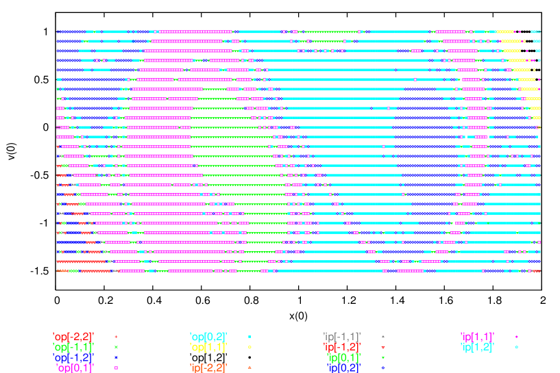
Figure 4: The figure shows the basins of attraction for bistable potential at $T=0.0005$. The dynamical states of the particle are represented by ip- (in-phase) and op- (out-of-phase) states with respect to applied periodic force. The wells and subwells in which the dynamical states exist are represented by the indices $l$ and $m$ within braces; e.g., op[0,1] indicates that the out-of-phase trajectory of the particle is in the (left) subwell-1 of the (initial) zeroth well of the potential.

When the underdamped particle moves along the potentials $U(x)(=\frac{2}{3}(\cos x+\cos 2x))$ and $U_{1}(x)(=-\sin x-F_{0}x)$ and driven by the external periodic field $F(t)$ the trajectories are essentially of just two kinds (states). The in-phase states correspond to trjectories $x(t)$ which lag behind $F(t)$ by a small phase $\phi_{1}$, whereas the out-of-phase states which lag behind $F(t)$ by a large phase $\phi_{2}$. Of course, $\phi_{1}$ and $\phi_{2}$ are approximate average values which weakly depend on the potential and the temperature. At low temperatures $\phi_{1}$ and $\phi_{2}$ essentially maintain the same values at each period of $F(t)$, Fig.3. The potential $U(x)$ has two similar subwells (Fig. 2) in a well, the trajectories in either subwell are just the same two states. Here, these in-phase and out-of-phase states are identified by the symbols ip($l,m$) and op($l,m$), respectively. $l$ indicates well number, for example, $l=0$ for the initial well, $l=-1(+1)$ for the first well to the left(right) of the initial well. $m$ indicates the subwell number: 1(2) for the left(right) subwell. These states are truly dynamical states. The basins of attraction of these states for the potential $U(x)$ is given in Fig. 4, as an illustration at temperature $T=.0005$.

Figure 5: Plot of $\overline{W}$ with $x(0)$ for $U_{1}(x)$ at $T=0.001$ (a), and $U(x)$ at $T=0.0005$ (b).

Figure 6: Plot of $\overline{W}$ with $x(0)$ for $U(x)$ at $T=0.001$ (a), $U_{1}(x)$ at $T=0.004$ (b).

At temperature $T=.0005$ the two states are quite stable and no transition between them could be observed. Though the potential barrier between any two consecutive wells have almost the same value for $U(x)$ and $U_{1}(x)$, their well bottoms are quite dissimilar and hence the input energy per period $\overline{W}$ are very different, Fig. 5. For $U_{1}(x)$, $\overline{W}$ are about 0.1 (in-phase) and 1.15 (out-of-phase), whereas for $U(x)$ they are about 0.04 (in-phase) and 0.32 (out-of-phase). Naturally, transitions between the two states for $U(x)$ occur at lower temperature than in case of $U_{1}(x)$, Fig. 6.

In the case of $U(x)$ by the temperature $T=0.001$ the indications of out-of-phase state going to the in-phase state, in a subwell, could be found and by $T=0.0015$ a substantial fraction of the out-of-phase states have jumped to the in-phase state. At $T=0.002$ all the out-of-phase states have made way to the in-phase state due to thermal fluctuations. Therefore, close to $T=0.002$ the system have the lowest average input energy $<\overline{W}>$ (or $<\overline{A}>$) per period of $F(t)$. And, from upward of $T=0.003$, the in-phase states begin to jump to the out-of-phase state. At $T=0.005$ even inter-subwell transitions could also be observed. The corresponding temperatures for the case of $U_{1}(x)$ are much higher.

Figure 7: Plot of $x(t)$ shows an inter-well transition for $U_{1}(x)$ at $T=0.01$ (a). A similar transition is seen for $U(x)$ at $T=0.23$ (b).

For the system with potential $U_{1}(x)$ the out-of-phase states begin going over to the in-phase state at around $T=0.004$ and the process completes at about $T=0.006$. The transition from the all-in-phase state to the out-of-phase state begins at about $T=0.009$. Interestingly, however, the inter-well transitions for $U_{1}(x)$ takes place at a much lower temperature (about $T=0.01$) than in case of the system with potential $U(x)$ which is only at about $T=0.23$, Fig. 7.

As stated earlier the periodic bistable potential $U(x)$ have essentially two states because the two subwells are energetically identical. In the case of the bistable washboard potential $U_{2}(x)(=U(x)-F_{0}x)$ the two subwells become dissimilar and the right subwell is energetically lower than the left one and we get two states corresponding to each subwell. However, the in-phase state in the left subwell becomes unstable for amplitude $\Delta F>0.19$ of the drive $F(t)$. Therefore, in our case, we have only one in-phase state to consider in the left subwell.

In case of $U_{2}(x)$, $\overline{W}$ is about 0.27 for the out-of-phase state in the left subwell (henceforth called subwell-1) and $\overline{W}$ for the two states in the other subwell (subwell-2) are about 0.03 (in-phase) and 0.37 (out-of-phase) at $T=0.0005$. By the temperature $T=0.001$ most of the (out-of-phase) states in subwell-1 go over to the states in subwell-2 and by $T=0.0015$ no states in subwell-1 survives. As the temperature is gradually increased the out-of-phase states in subwell-2 begin to jump over to the in-phase state in the same subwell and by $T=0.003$ we only have in-phase states in subwell-2 and $<\overline{W}>$ acquires a minimum value. By $T=0.009$ the particles begin to leave the in-phase state for the out-of-phase state in subwell-2 and we get a mixture of the two states in the same subwell. As the temperature is increased further, the transitions back and forth to subwell-1 begin at about $T=0.015$. Inter-well transitions begin, at a very slow rate, at about $T=0.08$, which is much higher than the corresponding temperature for the washboard potential $U_{1}(x)$ but lower than that for $U(x)$. The presence of two subwells in $U(x)$ and $U_{2}(x)$ makes the effective bottom of the wells flatter (smaller curvature) than in case of $U_{1}(x)$ and hence the inter-well transition rates smaller (see Eq. (3.5) below).

At $T>0.003$ ($T>0.01$) transitions from in-phase states to the out-of-phase states increase rapidly for $U(x)$ ($U_{1}(x)$), and consequently so does the $<\overline{W}>$, leading ultimately to the SR condition. Similar is the situation for $U_{2}(x)$.

III.2 Hysteresis loss and stochastic resonance

Figure 8: Plot of $\langle\overline{W}\rangle$ and SNR as a function of $T$ for the washboard potential $U_{1}(x)$.

Figure 9: Plot of $\langle\overline{W}\rangle$ and SNR as a function of $T$ for $U(x)$ (a) and $U_{2}(x)$ (b).

Figure 8 shows the variation of average input energy $<\overline{W}>$ or the average hysteresis loop area $<\overline{A}>$ and the signal-to-noise ratio (SNR) as a function of temperature for the washboard potential $U_{1}(x)$. The same functions are plotted for the potentials $U(x)$ and $U_{2}(x)$ in Fig. 9. $<\overline{W}>$ peaks at the temperatures $T=0.2,0.04$ and 0.08 for the potentials $U_{1}(x)$, $U(x)$ and $U_{2}(x)$, with peak values of about 0.36, 0.16, and 0.146, respectively. These maximum values of $<\overline{W}>$ lie between the $\overline{W}$ values of the in-phase and out-of-phase states for the corresponding potentials. There is, however, a remarkable difference between the nature of motion of particles at the temperature ($T_{SR}$) of maximum $<\overline{W}>$ for $U_{1}(x)$ on one hand and $U(x)$ and $U_{2}(x)$, on the other.

As the temperature $T$ goes through $T_{SR}\sim 0.2$ corresponding to maximum $<\overline{W}>$ , the particle feels the periodic nature of the potential $U_{1}(x)$ as the inter-well transitions are quite frequent, though not as frequent as the intra-well transitions between the in-phase to out-of-phase states. The particle motion is truly in a periodic potential implying the presence of stochastic resonance in the periodic potential $U_{1}(x)$. On the other hand, the particle has not yet begun the inter-well transitions (in $U(x)$) or have just started (in $U_{2}(x)$) as the temperature goes across the $<\overline{W}>$ maximum. Hence the particle does not feel the periodicity of the potentials but the presence of the two subwells. Therefore, the resonance effectively occurs in a single well with two subwells. However, the bistability in a well of the potentials is required for that to happen. Moreover, the existence of dynamical states of trajectories is necessary for the occurrence of $<\overline{W}>$ maximum at that low temperature, $T_{SR}=0.04$ for $U(x)$ and $T_{SR}=0.08$ for $U_{2}(x)$.

Consider the simple Smoluchowski limit of Kramers rateHanggi :

$$k=\frac{\omega_{0}\omega_{b}}{2\pi\gamma}\exp(\frac{-E_{b}}{T}),$$ (7)

where $\omega_{0}^{2}$ and $\omega_{b}^{2}$, respectively, are the curvatures at the bottom of the wells (subwells) and at the top of the barrier across the wells (subwells) of the potential $U_{1}(x)$ ($U(x)$ and $U_{2}(x)$). This rate calculation shows that $k^{-1}\sim 3450$ across the potential barrier between two consecutive wells of $U_{1}(x)$ ($T$=0.2, $\gamma=0.12$, $E_{b}=1.686$) and $k^{-1}\sim 47\times 10^{6}$ and 760 across the potential barrier between the two subwells in a well of the potentials $U(x)$ ($T$=0.04, $\gamma=0.12$, $E_{b}=0.75$) and $U_{2}(x)$ ($T$=0.08, $\gamma=0.12$, $E_{b}=0.618$), respectively.

Note that the periods $\tau=8.0,4.8$ and 4.8 of the drive field $F(t)$ taken, respectively, for the potentials $U_{1}(x),U(x)$ and $U_{2}(x)$ were too small compared to the calculated $k^{-1}$. Therefore, the observed SR cannot be considered as the conventional stochastic resonance following Ref.Kim . However, the resonance is brought about by the existence of and transition between the two dynamical (in-phase and out-of-phase) states of trajectories. The rates of these transitions are of the order of the period $\tau$ of the drive field. Viewed in this perspective of transition between the two dynamical states they, indeed, indicate SR. Moreover, the potential $U_{1}(x)$, at $T=T_{SR}$ a substantial number of inter-well transitions is observed. But in case of $U(x)$ and $U_{2}(x)$, inter-well transitions are seldom observed at $T=T_{SR}$. However, inter-subwell transitions are comparable in number to the transitions between the dynamical states at $T_{SR}$. SR nature of these transitions is further supported by the behaviour of input energy distributions P(W) across the temperature ($T_{SR}$) of maximum $<\overline{W}>$.

III.3 Input energy distribution and SR

Figure 10: Plot of $P(W)$ at different values of $T$ for $U_{1}(x)$ (a), $U(x)$ (b), and $U_{2}(x)$ (c). For small $T$, the distribution is bimodal for $U_{1}(x)$ and $U(x)$. However, $P(W)$ shows three peaks for $U_{2}(x)$.

The input energy distributions $P(W)$ have earlier been used in the discussion of SRSaikia ; Sahoo ; Jop ; PRE . $P(W)$, in the present case are shown in Fig. 10. At low temperatures, say $T=0.0005$, $P(W)$ shows the usual bimodal distribution for the potentials $U(x)$ and $U_{1}(x)$. The peaks occur exactly at $W=\overline{W}$ values shown in Fig. 5, corresponding to the $\overline{W}$ in the in-phase and out-of-phase states. Fig. 10 also shows $P(W)$ for the potential $U_{2}(x)$ exhibiting three peaks for the amplitude $\Delta F=0.2$ of $F(t)$. This is because, as mentioned earlier, the two subwells are not equivalent because of the finite average tilt $F_{0}=0.1$ in the potential $U_{2}(x)$. On general considerations one would expect four peaks. The four peak $P(W)$ appears only with $\Delta F<.19$. The three peak $P(W)$ instead occurs because of the instablity of the in-phase state in the subwell-1 for $\Delta F\geq.19$. Here again the peaks are centered at $W=\overline{W}$ values corresponding to the three dynamical states. The correspondence of the peaks of $P(W)$ and the dynamical states is thus unambiguous at low temperatures.

In Fig. 11 are shown $P(W)$ at various elevated temperatures. As the temperature is gradually increased two important common features could be readily observed: (i) the variation of the strength of the $P(W)$ peaks, and (ii) the intrusion of the in-phase peak into the negative $W$ domain and the appearance of a long negative $W$ tail of $P(W)$. The analysis of these two features provides a better understanding of SR in the three potential systems.

Figure 11: Plot of $P(W)$ at different values of $T$ for $U_{1}(x)$ (a), $U(x)$ (b), and $U_{2}(x)$ (c). At $T_{SR}$, $P(W)$ is on the verge of losing its multimodal character; at higher $T$ the distribution has a single peak structure.

For the potentials $U_{1}(x)$ and $U(x)$ the higher energy peak (corresponding to the out-of-phase state) first diminishes, disappears and then reappears, as the temperature is gradually increased. For $U_{2}(x)$, the peak of $P(W)$ corresponding to the out-of-phase state in the left subwell, i.e. op(0,1), first diasappears, and then the peak corresponding to op(0,2) too diasappears. As the temperature is increased further a broad peak (almost a plateau) appears roughly spanning the earlier two out-of-phase peaks. As the temperature is increased further the newly formed peaks begin merging with the sole in-phase peak (for $\Delta F=0.2$) and at the temperature $T_{SR}$ the out-of-phase peak is left only as a receding shoulder leaving no distinguishable trace of either a hump or a plateau. However, in the process the strength of the in-phase $P(W)$ peak also diminishes. This can be seen in either of the two ways: (i) by fitting the in-phase $P(W)$ peak by a Gaussian and calculating its area and (ii) by finding the ratio of the number of points in the stroboscopic (Poincaré) plots falling in the in-phase region to the total number of points.

The fraction (contribution) of in-phase states in the trajectory reduces from 1 (at $T=T_{min}\sim 0.02,0.003$ and 0.003 for $U_{1}(x)$, $U(x)$ and $U_{2}(x)$, respectively, corresponding to the respective minimum of $<\overline{W}>$) gradually and becomes almost equal to 0.5 at the temperature $T_{SR}$ of maximum $<\overline{W}>$ ($T_{SR}\sim 0.2,0.04$ and 0.08 for $U_{1}(x)$, $U(x)$ and $U_{2}(x)$, respectively), Fig. 12. At this temperature, it becomes hard to clearly distinguish the regions of in-phase and out-of-phase states of trajectories, just as in the liquid-gas system at the critical temperature. The temperature of maximum $<\overline{W}>$ is said to fall in the region of kinetic phase transitionsDykman2 .

The second important feature of $P(W)$ is its intrusion into the negative $W$ region. As mentioned earlier it has two components: (i) a systematic broadening of the in-phase peak of $P(W)$ and spilling over to $W<0$ region and (ii) the emergence of a long $W<0$ tail. The former happens at a temperature much lower than the temperature at which the $W<0$ tail begins to emerge. The phase lag $\phi_{1}$ in case of in-phase is small ($-\phi_{1}\sim 0.1\pi,0.08\pi$ and $0.08\pi$, respectively for the $U_{1}(x)$, $U(x)$ and $U_{2}(x)$ potentials). Also the in-phase $P(W)$ peak is centered close to $W\geq 0$. As the temperature is increased the fluctuations in the value of $\phi_{1}$ occur leading sometime to make $\phi_{1}>0$. In other words, the thermal effect, makes $x(t)$ occasionally lead the forcing $F(t)$. Thus, a few individual HLAs acquire a sign opposite to what is observed in the usual case when causality is respected. Therefore, occasionally, $W$ becomes negative and the in-phase peak of $P(W)$ broadens into the $W<0$ region. This process continues and becomes more evident as the temperature is increased.

Analyses of the trajectories $x(t)$ and the accompanying hysteresis loops $x(F(t))$ reveal that the violation of causality (leading to $W<0$) occurs during the transitions between the dynamical (in-phase and out-of-phase) states. In these situations the magnitude of negative $W$ (hysteresis loop area with opposite sign) often becomes very large. The origin of negative tail of $P(W)$ lies in these transitions between the dynamical phases. Since, before the temperature at which $<\overline{W}>$ becomes minimum at most one (out-of-phase to in-phase) transition occurs in the entire history of any trajectory spanning about $10^{5}$ periods of $F(t)$ the negative tail of $P(W)$ does not show up till the temperature $T_{min}$ of minimum $<\overline{W}>$ ($T_{min}\sim 0.02,0.003$ and 0.003 for $U_{1}(x)$, $U(x)$ and $U_{2}(x)$, respectively).

Figure 12: The figure shows the plot of the fraction (ratio) of time spent by the particle in its in-phase state of trajectories as a function of temperature $T$, for the potentials $U(x)$ ($T_{SR}=0.04$), $U_{2}(x)$ ($T_{SR}=0.08$), and $U_{1}(x)$ ($T_{SR}=0.2$).

As the temperature is gradually increased further, the transitions, initially from the (all) in-phase to the out-of-phase states take place and the high energy peak (plateau) reappears. Thereafter, transitions in both directions become more and more frequent ultimately causing the newly emerged high energy (out-of-phase) peak (plateau) to merge with the in-phase peak at the resonance temperature $T_{SR}$. The increase of negative tail of $P(W)$ goes hand in hand with increasing $T$. At temperatures $T\geq T_{SR}$ the transition regions dominate over the regions of in-phase and out-of-phase dynamical states. At these temperatures the increasing long negative tail and the ever broadening in-phase peak of $P(W)$ bring down $<\overline{W}>$ from its maximum value at ($T_{SR}$). Note that on the average causality is always respected and $<\overline{W}>$ never becomes negative.

III.4 Average amplitude and phase of hysteresis loops

Figure 13: Plot of $x_{0}$ and $-\overline{\phi}$ (insets) with $T$ for $U_{1}(x)$ (a), for $U(x)$ (b), and for $U_{2}(x)$) (c).

The average hysteresis loops $<\overline{x}(F(t_{i}))>$ are calculated using Eq. (3.4). Since the amplitude $\Delta F$ of the external drive $F(t)=\Delta F\cos(\frac{2\pi}{\tau}t)$ (=0.2) is much smaller than the periodic barrier heights ($\sim 2.0$) between two consecutive wells, the amplitude $x_{0}$ of the average response $<\overline{x}(F(t_{i}))>$ is small and the relation $<\overline{x}(F(t_{i}))>=x_{0}\cos(\frac{2\pi}{\tau}t+\overline{\phi})$, with $t=n\tau+t_{i}$, is found to follow quite well for all three potentials at low temperatures. However, at higher temperatures the relation serves reasonably well for the potential $U_{1}(x)$, and only approximately for $U(x)$ and $U_{2}(x)$.

The amplitude $x_{0}$ and phase $|\overline{\phi}|$ acquire their respective minima at the temperature $T_{min}$ of minimum $<\overline{W}>$ corresponding to the sole dynamical (in-phase) state, Fig. 13. At this temperature $\overline{\phi}\sim\phi_{1}$. As the temperatrure is gradually increased from $T=T_{min}$ $x_{0}$ peaks at $T\sim T_{SR}$. However, $\overline{\phi}$ shows a monotonic behaviour. At these temperatures $|\phi_{1}|<|\overline{\phi}|<|\phi_{2}|$ because the trajectories consist of a mixture of in-phase and out-of-phase states. The variation of $\overline{\phi}$ is similar to what is reported earlierLGamma and does not show a peakDykman1 .

IV Discussion and conclusion

The existence of two dynamical states in a sinusoidally driven (under)damped system is quite special to periodic potentials. The (quadratic) harmonic potentials or the (quartic) Landau potentials show only one (in-phase) state. The periodic nature of the potentials allows the particle to explore (in space) regions of high nonlinearity. The high nonlinearity of periodic potentials appears to be responsible for the occurrence of these two states (especially the additional high amplitude out-of-phase state) in a well in a sinusoidal potential or in a subwell in the bistable periodic or washboard potential.

The investigation of dependence of the existence of two dynamical states on the amplitude of the drive field could also be of interest in periodic potentials. As observed earlier, the in-phase state in the left subwell of the potential $U_{2}(x)$ disappears for $\Delta F>0.19$. However, if $\Delta F$ is chosen to be too small the particle may not have the opportunity to explore the highly nonlinear regions of the potential and the out-of-phase trajectories may disappear. Therefore, the choice of $\Delta F$ too is crucial for the study of SR in these potentials.

In the conventional SR it is the bistability of the potential that plays a crucial role. In the present periodic (or washboard) potential case SR is brought about by the bistability (or multistability) of the states of trajectories in a well (subwell) together with the adjacent wells (subwells) of the potential. Moreover, if the system is initially prepared in a given well of a double-well potential the conventional SR occurs when the probability distribution of particles becomes equal in both the wells in a finite (small) time (typically, of the order of the period of the drive field). In other words, the rate of passages across the potential barrier between the two wells becomes equal. Exactly similar is the condition in the periodic potential cases considered in the present work. The ratio of time spent by the particle in either of the two states of trajectories to the total time reaches 0.5 as the temperature rises to $T_{SR}$, Fig. 12.

In order to observe SR in the ‘periodic’ potentials discussed above it is necessary to choose the period $\tau$ of the drive field judiciously. SR occurs in a narrow ‘window’ of frequency $\omega$ ($\omega=\frac{2\pi}{\tau}$): approximately, [$7.8<\tau<9.8$] for the potential $U_{1}(x)$ and [$4.8\leq\tau<10.6$] for $U(x)$ and [$4.0<\tau<9.8$] for the potential $U_{2}(x)$. The lower limit of the $\tau$-window is sharp. However, the upper limit is not well demarcated. The $T_{SR}$ increases monotonocally with $\tau$. Here the upper limit of the $\tau$-window is arbitrarily put so that $T_{SR}=0.7$. $T_{SR}=0.7$ is a large temperature and is comparable to the potential barrier $\sim 2$ between two adjacent wells of the potentials. Consequently, $<\overline{W}>(T)$ peak becomes broader with increasing $\tau$. However, the numerical results for the potentials $U(x)$ and $U_{2}(x)$ are expected to improve if $\tau$ is chosen larger than the value 4.8. Indeed, the preliminary results show that when $\tau$ is chosen somewhat larger than 4.8 even frequent inter-well transitions could be observed around $T_{SR}$ for the potentials $U(x)$ and $U_{2}(x)$. This effectively addresses the earlier limitation of particle motion being confined to a single well. This provides further support to the thesis of the presence of SR in these ‘periodic’ potentials.

MCM acknowledges partial financial support from BRNS, DAE, India under Project No. 2009/37/17/BRNS/1959. Partial financial support from the UGC, India, in the form of Special Assistance Program to the Department of Physics, NEHU, Shillong, India is acknowledged.

References

- (1) R. Benzi, A. Sutera, and A. Vulpiani J. Phys. A 14, L453 (1981).
- (2) S. Fauve, and F. Heslot, Phys. Lett. A 97, 5 (1983).
- (3) B. McNamara, K. Wiesenfeld, and R. Roy, Phys. Rev. Lett. 60, 2626 (1988).
- (4) J.K. Douglass, L. Wilkens, E. Pantazelou, and F. Moss, Nature 365, 337 (1993).
- (5) K. Wiesenfeld, and F. Moss, Nature 373, 33 (1995).
- (6) L. Gammaitoni, P. Hänggi, P. Jung, and F. Marchesoni, Rev. Mod. Phys. 70, 223 (1998).
- (7) T. Wellens, V. Shatokhin, and A. Buchleitner, Rep. Prog. Phys. 67, 45 (2004).
- (8) R.N. Mantegna, and B. Spagnolo, Phys. Rev. E 49, R1792 (1994).
- (9) K. Murali, S. Sinha, W.L. Ditto, A.R. Bulsara, Phys. Rev. Lett. 102, 104101 (2009).
- (10) R.L. Badzey, and P. Mohanty, Nature 437, 995 (2005).
- (11) J.J. Collins, T.T. Imhoff, and P. Grigg, J. Neurophysiology 76, 642 (1996).
- (12) B.J. Gluckman, T.I. Netoff, E.J. Neel, W.L. Ditto, M.L. Spano, S.J. Schiff, Phys. Rev. Lett. 77, 4098 (1996).
- (13) E. Simonotto, M. Riani, C. Seife, M. Roberts, J. Twitty, and F. Moss, Phys. Rev. Lett. 78, 1186 (1997).
- (14) D. Tabarelli, A. Vilardi, C. Begliomini, F. Pavani, M. Turatto, and L. Ricci, Eur. Phys. J. B 69, 155 (2009).
- (15) B. McNamara, and K. Wiesenfeld, Phys. Rev. A 39, 4854 (1989).
- (16) Y.W. Kim, and W. Sung, Phys. Rev. E 57, R6237 (1998).
- (17) N.G. Stocks, P.V.E. McClintock, and S.M. Soskin, Europhys. Lett. 21, 395 (1993); N.G. Stocks, N.D. Stein, and P.V.E. McClintock, J. Phys. A: Math. Gen. 26, L385 (1993).
- (18) M.I. Dykman, D.G. Luchinsky, R. Mannella, P.V.E. McClintock, N.D. Stein, and N.G. Stocks J. Stat. Phys. 70, 479 (1993).
- (19) A.P. Graham, F. Hofmann, J.P. Toennies, L.Y. Chen, and S.C. Ying, Phys. Rev. B 56, 10567 (1997); D.C. Senft, and G. Ehrlich, Phys. rev. Lett. 74, 294 (1995).
- (20) I.Kh. Kaufman, D.G. Luchinsky, P.V.E. McClintock, S.M. Soskin, and N.D. Stein, Phys. Lett. A 220, 219 (1996).
- (21) A. Borone, and G. Paterno, Physics and Applications of the Josephson Effect, John-Wiley & Sons, 1982.
- (22) H. Risken, The Fokker-Plank Equation, Springer Verlag, 1989.
- (23) S. Saikia, A.M. Jayannavar, and M.C. Mahato, Phys. Rev E83, 061121 (2011).
- (24) M.C. Mahato, and S.R. Shenoy, Phys. Rev. E 50, 2503 (1994).
- (25) T. Iwai, Physica A 300, 350 (2001).
- (26) E. Heinsalu, M. Patriarca, and F. Marchesoni, Eur. Phys. J. B 69, 19 (2009).
- (27) S. Saikia, R. Roy, and A.M. Jayannavar, Phys. Lett. A 369, 367 (2007).
- (28) M. Sahoo, S. Saikia, M.C. Mahato, and A.M. Jayannavar, Physica A 387, 6284 (2008).
- (29) P. Jop, A. Petrosyan, and S. Ciliberto, EPL 81, 50005 (2008).
- (30) M. Evstigneev, P. Reimann, C. Schmitt, and C.Bechinger, J. Phys.: Condens. Matter 17, S3795 (2005).
- (31) P. Jung, and F. Marchesoni, Unpublished.
- (32) See for example, M. Lakshmanan, and S. Rajasekar, Nonlinear Dynamics, Springer Verlag, Heidelberg, 2003.
- (33) R. Mannella, A Gentle Introduction to the Integration of Stochastic Differential Equations. In : Stochastic Processes in Physics, Chemistry, and Biology. Edited by J. A. Freund and T. Pöschel, Lecture Notes in Physics, vol. 557, 353. Springer, Berlin, 2000.
- (34) K. Sekimoto, J. Phys. Soc. Jpn. 66, 1234 (1997).
- (35) L. Gammaitoni, F. Marchesoni, M. Martinelli, L. Pardi, and S. Santucci, Phys. Lett. A 158, 449 (1991).
- (36) M.I. Dykman, R. Mannella, P.V.E. McClintock, and N.G. Stocks, Phys. Rev. Lett. 68, 2985 (1992); L. Gammaitoni, and F. Marchesoni, Phys. Rev. Lett. 70, 873 (1993); M.I. Dykman, R. Mannella, P.V.E. McClintock, and N.G. Stocks, Phys. Rev. Lett. 70, 874 (1993).
- (37) P. Hänggi, P. Talkner, and M. Borkovec, Rev. Mod. Phys. 62, 251 (1990).
- (38) M.I. Dykman, R. Mannella, P.V.E. McClintock, and N.G. Stocks, Phys. Rev. Lett. 65, 48 (1990).