A Coding Theoretic Approach for Evaluating Accumulate Distribution on Minimum Cut Capacity of Weighted Random Graphs

Abstract

The multicast capacity of a directed network is closely related to the $s$-$t$ maximum flow, which is equal to the $s$-$t$ minimum cut capacity due to the max-flow min-cut theorem. If the topology of a network (or link capacities) is dynamically changing or have stochastic nature, it is not so trivial to predict statistical properties on the maximum flow. In this paper, we present a coding theoretic approach for evaluating the accumulate distribution of the minimum cut capacity of weighted random graphs. The main feature of our approach is to utilize the correspondence between the cut space of a graph and a binary LDGM (low-density generator-matrix) code with column weight 2. The graph ensemble treated in the paper is a weighted version of Erdős-Rényi random graph ensemble. The main contribution of our work is a combinatorial lower bound for the accumulate distribution of the minimum cut capacity. From some computer experiments, it is observed that the lower bound derived here reflects the actual statistical behavior of the minimum cut capacity.

I Introduction

Rapid growth of information flow over a network such as a backbone network for mobile terminals requires efficient utilization of full potential of the network. In a multicast communication scenario, it is well known that an appropriate network coding achieves its multicast capacity. Emergence of the network coding have broaden network design strategies for efficient use of wired and wireless networks [16].

The multicast capacity of a directed graph is closely related to the $s$-$t$ maximum flow, which is equal to the $s$-$t$ minimum cut capacity due to the max-flow min-cut theorem [15]. The topology of a network and the assignment of the link capacities determine the $s$-$t$ minimum cut capacity of a network.

If a network is fixed, the corresponding $s$-$t$ maximum flow of the network can be efficiently evaluated by using Ford-Fulkerson algorithm [15]. However, if the topology of a network (or link capacities) is dynamically changing or have stochastic nature, it is not so trivial to predict statistical properties on the maximum flow. For example, in a case of wireless network, the link capacities may fluctuate because of the effect of time-varying fading. Another example is an ad-hoc network whose link connections are stochastically determined.

In order to obtain an insight for the statistical property of the min-cut capacity for such random networks, it is natural to investigate the statistical properties of a random graph ensemble. Such a result may unveil typical behaviors of minimum cut capacity (or maximum flow) for given parameters, such as the number of vertices and edges.

Several theoretical works on the maximum flow of random graphs (i.e., graph ensembles) have been made. In a context of randomized algorithms, Karger showed a sharp concentration result for maximum flow in the asymptotic regime [11]. Ramamoorthy et al. presented another concentration result; the network coding capacities of weighted random graphs and weighted random geometric graphs concentrate around the expected number of nearest neighbors of the source and the sinks [12]. These concentration results indicate an asymptotic property of the maximum flow of random networks. Wang et al. shows statistical property of the maximum flow in an asymptotic setting as well. They discussed the random graph with Bernoulli distributed weights [10].

In this paper, we present a coding theoretic approach for evaluating the accumulate distribution of the minimum-cut capacity of weighted random graphs. This approach is totally different from those used in the conventional works. The basis of the analysis is the correspondence between the cut space of an undirected graph [5] and a binary LDGM (low-density generator-matrix) code with column weight 2. Yano and Wadayama presented that an ensemble analysis for a class of binary LDGM codes with column weight 2 for the network reliability problem [13]. This paper extends the idea in [13] to weighted graph ensembles. We focus on a weighted version of Erdős-Rényi random graph ensemble [4] in this paper.

II Preliminaries

In this section, we first introduce several basic definitions and notation used throughout the paper. Then, the cut-set weight distribution will be discussed.

II-A Notation and definitions

A graph $G=(V,E)$ is a pair of a vertex set $V=\{v_{1},\ldots,v_{k}\}$ and an edge set $E=\{e_{1},\ldots,e_{n}\}$ where $e_{j}=(u,v),u,v\in V$ is an edge. If $e_{j}=(u,v)$ is not an ordered pair, i.e., $(u,v)=(v,u)$, the graph $G$ is called an undirected graph. Otherwise, i.e., $(u,v)$ is an ordered pair, $G$ is a directed graph. The two vertices connecting an edge $e\in E$ are referred to as the end points of $e$. If an edge $e=(u,u)$ has the identical end points, $e$ is called a self-loop.

If real valued function $w:E\rightarrow\mathbb{R}_{\geq 0}$ is defined for an undirected graph $G=(V,E)$, the triple $(V,E,w)$ is considered as a weighted graph. The set $\mathbb{R}_{\geq 0}$ represents the set of non-negative real numbers. In our context, the weight function $w$ represents the link capacity for each edge.

Assume that a weighted undirected graph $G=(V,E,w)$ is given. A non-overlapping bi-partition $V=X\cup(V\backslash X)$ is called a cut where $X$ is a non-empty proper subset of $V(X\neq V)$. The set of edges bridging $X$ and $V\backslash X$ is referred to as the cut-set corresponding to the cut of $(X,V\backslash X)$. The cut weight of $X$ is defined as $\sum_{u\in X,v\in V\backslash X}w(u,v).$

II-B Random graph ensemble

In the following, we will define an ensemble of weighted undirected graphs. The graph ensemble is based on Erdős-Rényi random graph ensemble. Let $k(k\geq 1)$ be the number of labeled vertices and $n(1\leq n\leq k(k-1)/2)$ be the number of labeled undirected edges. The vertices are labeled from $1$ to $k$ and the edges are labeled from $1$ to $n$.

For any adjacent vertices, a single edge is only allowed. It is assumed that each edge has own integer weight; namely, a weight $w_{i}\in[1,q](i\in[1,n])$ is assigned to the edge with label $i$, which is denoted by the $i$th edge. The notation $[a,b]$ denotes the set of consecutive integers from $a$ to $b$. The set $R_{k,n}^{q}$ denotes the set of all undirected weighted graphs with $k$-vertices and $n$-edges satisfying the above assumption.

For any $G\in R_{k,n}^{q}$, the sets of vertices and edges are denoted by $V(G)$ and $E(G)$, respectively. In a similar way, $w_{i}(G)$ is defined as the weight of $i$th edge of $G$.

It is evident that the cardinality of $R_{k,n}^{q}$ is given by

$$|R_{k,n}^{q}|=n!{{k\choose 2}\choose n}q^{n}.$$ (1)

We here assign the probability

$$P(G)=\frac{1}{n!{{k\choose 2}\choose n}}\mu(w_{1}(G))\mu(w_{2}(G))\cdots\mu(w_{n}(G))$$ (2)

for $G\in R^{q}_{k,n}$ where $\mu$ is a discrete probability measure defined over $[1,q]$; namely, it satisfies

$$\sum_{w\in[1,q]}\mu(w)=1\mbox{ and }\forall w\in[1,q],\mu(w)\geq 0.$$ (3)

The pair $(R_{k,n}^{q},P)$ defines an ensemble of random graphs and it is denoted by ${\cal E}$.

II-C Incidence matrix

For $G\in R^{q}_{k,n}$, the incidence matrix of $G$, denoted by $M(G)\in\{0,1\}^{k\times n}$, is defined as follows:

$$M(G)_{i,j}=\left\{\begin{array}[]{ll}1,&\mbox{if $i$-th vertex connects to $j$-th edge}\\ 0,&\mbox{otherwise},\\ \end{array}\right.$$ (4)

where $M(G)_{i,j}$ is the $(i,j)$-element of $M(G)$. If $G$ is connected, then the rank (over $\mathbb{F}_{2}$) of $M(G)$ is $k-1$. The row space (over $\mathbb{F}_{2}$) of $M(G)$ coincides with the set of all possible incidence vectors of cut-sets of $G$.

II-D Cut weight distribution

For a given undirected graph, we can enumerate the number of cut-sets with cut weight $w$. The cut weight distribution of $G$ by

$$B_{w}(G)=\sum_{E\subset E(G)}\mathbb{I}[E\mbox{ is a cut-set of }G,\mbox{cut weight is }w]$$ (5)

for positive integer $w$. The function $\mathbb{I}[\cdot]$ is the indicator function that takes value 1 if the condition is true; otherwise it takes value 0. This cut weight distribution can be regarded as an analog of the weight distribution of the binary linear code defined by the incidence matrix of a given undirected graph.

For ensemble analysis, it is convenient to introduce another form of the weight distribution. The detailed cut weight distribution $A_{u,v.w}:R_{k,n}^{q}\rightarrow\mathbb{Z}_{\geq 0}$ is defined by

$$A_{u,v,w}(G)$$ (6)

$$=\sum_{m\in Z^{(k,u)}}\sum_{c\in Z^{(n,v)}}\mathbb{I}\left[mM(G)=c,\sum_{i=1}^{n}c_{i}w_{i}(G)=w\right],$$

for $u\in[1,k-1],v\in[0,n]$. The set of constant weight binary vectors $Z^{(a,b)}$ is defined as

$$Z^{(a,b)}=\{x\in\{0,1\}^{a}:w_{H}(x)=b\}.$$ (7)

The function $w_{H}(\cdot)$ represents the Hamming weight. Assume that the cardinality of the cut is $v$ and that the size of $X\subset E$ is $u$. Under this condition, the function $A_{u,v,w}(G)$ represents the number of cuts with the cut weight $w$. It should be noted that the one-to-one correspondence between the cut space and the set of incident vectors of the cuts are implicitly used in the definition of $A_{u,v,w}(G)$.

The following lemma indicates the relationship between $A_{u,v,w}$ and $B_{w}(G)$.

Lemma 1

For $G\in R_{k,n}^{q}$, the cut weight distribution $B_{w}(G)$ can be upper bounded by

$$B_{w}(G)\leq\frac{1}{2}\sum_{u=1}^{k-1}\sum_{v=0}^{n}A_{u,v.w}(G),$$ (8)

for $w\in\mathbb{Z}_{\geq 0}$. The notation $\mathbb{Z}_{\geq 0}$ represents the set of non-negative integers.

Proof:

Let

$$S(G)=\{c=mM(G)\in\mathbb{F}_{2}^{n}\mid m\in\mathbb{F}_{2}^{k}\backslash\{0^{k},1^{k}\}\}.$$

The cut weight distribution $B_{w}(G)$ can be rewritten as follows.

$$B_{w}(G) = \sum_{E\subset E(G)}\mathbb{I}[E\mbox{ is a cut-set of }G,\mbox{cut capacity is }w]$$ (9)

$$= \sum_{c\in S(G)}\mathbb{I}\left[\sum_{i=1}^{n}c_{i}w_{i}(G)=w\right].$$

The second equality is due to the fact that the row space of $M(G)$ equals the set of all possible cut-set vectors of $G$. It is evident that

$$|\{m\in\mathbb{F}_{2}^{k}\mid m\neq 0^{k},m\neq 1^{k},c=mM(G)\}|\geq 2$$

holds for any $c\in S(G)$. This implies that

$$\sum_{c\in S(G)}h(c)\leq\frac{1}{2}\sum_{m\in\{0,1\}^{k}\backslash\{0^{k},1^{k}\}}\sum_{c\in\{0,1\}^{n}}h(c)\mathbb{I}\left[c=mM(G)\right]$$ (10)

holds for any real-valued function $h:\{0,1\}^{n}\rightarrow\mathbb{R}$. Substituting (10) into (9), we obtain

$$B_{w}(G) \leq \frac{1}{2}\sum_{m\in\{0,1\}^{k}\backslash\{0^{k},1^{k}\}}\sum_{c\in\{0,1\}^{n}}\mathbb{I}\left[c=mM(G)\right]$$ (11)

$$\times \mathbb{I}\left[\sum_{i=1}^{n}c_{i}w_{i}(G)=w\right]$$

$$= \frac{1}{2}\sum_{u=1}^{k-1}\sum_{v=0}^{n}A_{u,v.w}(G).$$

∎

III Ensemble average of cut weight distribution

In this section, we discuss the average of $A_{u,v,w}(G)$ over the ensemble ${\cal E}$. This analysis is very similar to the derivation of the average weight distribution of LDGM codes with column weight 2.

III-A Preparation

In the following, the expectation operator ${\sf E}$ is defined as

$${\sf E}[f(G)]=\sum_{G\in R_{k,n}^{q}}P(G)f(G),$$ (12)

where $f$ is any real-valued function defined on $R_{k,n}^{q}$. The next lemma plays a key role to derive a closed form the average cut set weight distribution.

Lemma 2

Assume that $m^{*}\in\{0,1\}^{k}$ and $c^{*}\in\{0,1\}^{n}$ satisfies $w_{H}(m^{*})=u$ and $w_{H}(c^{*})=v$ where $u\in[1,k-1]$ and $v\in[0,n]$. The following equality

$${\sf E}\left[\mathbb{I}\left[m^{*}M(G)=c^{*},\sum_{i=1}^{n}c_{i}^{*}w_{i}(G)=w\right]\right]$$

$$= \frac{1}{{n\choose v}{{k\choose 2}\choose n}}{u(k-u)\choose v}{{k\choose 2}-u(k-u)\choose n-v}[x^{w}]f(x)^{v}$$

holds. The function $f(x)$ is defined by

$$f(x)=\sum_{i=1}^{q}\mu(i)x^{i}.$$ (14)

The term $[x^{w}]f(x)^{v}$ represents the coefficient of $x^{w}$ in $f(x)^{v}$.

Proof:

Due to the symmetry of the ensemble, we can assume that the first $u$-elements of $m^{*}$ are one and the rests are zero without loss of generality. In a similar manner, $c^{*}$ is assumed to be the binary vector such that first $v$-elements are one and the rests are zero.

In the following, we will count the number of labeled graphs satisfying $m^{*}M(G)=c^{*}$ by counting the number of binary incidence matrices satisfying the above condition. Let $M(G)=\left(f_{1}\ f_{2}\ \cdots f_{n}\right)$ where $f_{i}$ is the $i$th column vector of $M(G)$. Since $M(G)$ is an incidence matrix, the column weight of $f_{i}$ is $w_{H}(f_{i})=2$ for $i\in[1,n]$. From the assumptions described above, we have

$$m^{*}f_{i}=\left\{\begin{array}[]{ll}1,&i\in[1,v]\\ 0,&i\in[v+1,n].\\ \end{array}\right.$$ (15)

We then count the number of allowable combinations of $(f_{1},f_{2},\ldots,f_{n})$ satisfying (15). Let

$$A=\{f\in\{0,1\}^{k}\mid m^{*}f=1,w_{H}(f)=2\}.$$ (16)

The cardinality of $A$ is given by $|A|=u(k-u)$ because a non-zero component of $f$ needs to have an index within $[1,u]$ and another non-zero component has an index in the range $[u+1,k]$. This observation leads to the number of possibilities for $(f_{1},f_{2},\ldots,f_{v})$ which is given by $v!{u(k-u)\choose v}.$ The remaining $n-v$ columns, $(f_{v+1},\ldots,f_{n})$, should be taken from the set $\{f\in\{0,1\}^{k}\mid w_{H}(f)=2\}\backslash A$. Thus, the number of possibilities for such choice is $(n-v)!{{k\choose 2}-u(k-u)\choose n-v}.$ In summary, the number of allowable combinations of $(f_{1},f_{2},\ldots,f_{n})$ denoted by $S$ is given by

$$S=v!(n-v)!{u(k-u)\choose v}{{k\choose 2}-u(k-u)\choose n-v}.$$ (17)

We are now ready to derive the claim of this lemma. To simplify the notation, the cut weight is denoted by $\psi(c)=\sum_{i=1}^{n}c_{i}w_{i}(G).$ The left hand side of (LABEL:closed) can be rewritten as follows:

$${\sf E}[\mathbb{I}[m^{*}M(G)=c^{*},\psi(c^{*})=w]$$

$$= \sum_{G\in R_{k,n}^{q}}P(G)I[m^{*}M(G)=c^{*},\psi(c^{*})=w]$$

$$= \frac{1}{n!{{k\choose 2}\choose n}}\sum_{G\in R_{k,n}^{q}}\left(\prod_{i\in[1,n]}\mu(w_{i}(G))\right)$$

$$\times \mathbb{I}[m^{*}M(G)=c^{*},\psi(c^{*})=w]$$

$$= \frac{S}{n!{{k\choose 2}\choose n}}\sum_{\stackrel{{\scriptstyle u_{1}+\cdots+u_{q}=v,}}{{u_{1}+2u_{2}+\cdots qu_{q}=w}}}\left(\prod_{i\in[1,q]}\mu(i)^{u_{i}}\right)\frac{v!}{u_{1}!u_{2}!\cdots u_{q}!}$$

$$= \frac{v!(n-v)!}{n!{{k\choose 2}\choose n}}{u(k-u)\choose v}{{k\choose 2}-u(k-u)\choose n-v}[x^{w}]f(x)^{v}.$$

The last equality is due to (17). ∎

The following lemma provides the ensemble average ${\sf E}[A_{u,v,w}(G)]$, which is a natural consequence of Lemma 2.

Lemma 3

The expectation of $A_{u,v,w}(G)$ is given by

$${\sf E}[A_{u,v,w}(G)]\hskip 170.71652pt$$

$$=\frac{1}{{{k\choose 2}\choose n}}{k\choose u}{u(k-u)\choose v}{{k\choose 2}-u(k-u)\choose n-v}[x^{w}]f(x)^{v},$$ (19)

where $u\in[1,k-1],v\in[0,n],w\in\mathbb{Z}_{>0}$.

Proof:

The expectation of $A_{u,v,w}(G)$ can be simplified as follows:

$${\sf E}[A_{u,v,w}(G)]$$ (20)

$$= {\sf E}\left[\sum_{m\in Z^{(k,u)}}\sum_{c\in Z^{(n,v)}}\mathbb{I}[mM(G)=c,\psi(c)=w]\right]$$

$$= \sum_{m\in Z^{(k,u)}}\sum_{c\in Z^{(n,v)}}{\sf E}\left[\mathbb{I}[mM(G)=c,\psi(c)=w]\right]$$

$$= {k\choose u}{n\choose v}{\sf E}\left[\mathbb{I}[m^{*}M(G)=c^{*},\psi(c^{*})=w]\right].$$

The last equality is due to the symmetry of the ensemble. The binary vectors $m^{*}\in\{0,1\}^{k}$ and $c^{*}\in\{0,1\}^{n}$ are arbitrary vectors satisfying $w_{H}(m^{*})=u$ and $w_{H}(c^{*})=v$. Substituting (LABEL:closed) in the previous Lemma into (20), we obtain the claim of this lemma. ∎

III-B Upper bound on average cut weight distribution

In order to investigate statistical properties of the minimum cut weight, it is natural to study the tail of the average cut weight distribution. The following theorem provides an upper bound on average cut weight distribution that is the basis of our analysis.

Theorem 1

The expectation of $B_{w}(G)$ over ${\cal E}$ can be upper bounded by

$${\sf E}[B_{w}(G)] \leq \frac{1}{2{{k\choose 2}\choose n}}\sum_{u=1}^{k-1}{k\choose u}\sum_{v=0}^{n}{u(k-u)\choose v}$$ (21)

$$\times {{k\choose 2}-u(k-u)\choose n-v}[x^{w}]f(x)^{v}$$

for $w\in\mathbb{Z}_{\geq 0}$.

Proof:

Due to Lemma 1, we immediately have

$${\sf E}[B_{w}(G)] \leq {\sf E}\left[\frac{1}{2}\sum_{u=1}^{k-1}\sum_{v=0}^{n}A_{u,v.w}(G)\right]$$ (22)

$$= \frac{1}{2}\sum_{u=1}^{k-1}\sum_{v=0}^{n}{\sf E}\left[A_{u,v.w}(G)\right].$$ (23)

Substituting the left hand side of the equality in Lemma 3 into the last equation gives the claim of the theorem. ∎

III-C Accumulate cut distribution

Let us define the accumulate cut weight of $G$, $C_{\delta}(G)$, by

$$C_{\delta}(G)=\sum_{w=0}^{\delta-1}B_{w}(G),$$ (24)

where $\delta$ is a non-negative integer. If $C_{\delta}(G)$ is zero, the graph $G$ does not contain a cut with weight smaller than $\delta$. This implies that $\lambda(G)\geq\delta$ in such a case, thus we have

$$Pr[\lambda(G)\geq\delta] = Pr[C_{\delta}(G)=0]$$ (25)

$$= 1-Pr[C_{\delta}(G)\geq 1].$$

The second equality is due to the non-negativity of $C_{\delta}(G)$. The probability $Pr[\lambda(G)\geq\delta]$ can be considered as the accumulate probability distribution for the minimum cut capacity:

$$Pr[\lambda(G)\geq\delta]=\sum_{G\in R_{k,n}^{q}}P(G)\mathbb{I}[\lambda(G)\geq\delta].$$ (26)

The following theorem is the main contribution of this work.

Theorem 2

Assume that an ensemble ${\cal E}$ is given. The probability $Pr[\lambda(G)\geq\delta]$ can be lower bounded by

$$Pr[\lambda(G)\geq\delta] \geq 1-\frac{1}{2{{k\choose 2}\choose n}}\sum_{w=0}^{\delta-1}\sum_{u=1}^{k-1}{k\choose u}\sum_{v=0}^{n}{u(k-u)\choose v}$$ (27)

$$\times {{k\choose 2}-u(k-u)\choose n-v}[x^{w}]f(x)^{v}$$

for $\delta\in\mathbb{Z}_{\geq 0}$.

Proof:

Markov inequality

$$Pr[C_{\delta}(G)\geq 1]\leq{\sf E}[C_{\delta}(G)]$$ (28)

provides an lower bound on $Pr[\lambda(G)\geq\delta]$:

$$Pr[\lambda(G)\geq\delta] = 1-Pr[C_{\delta}(G)\geq 1]$$ (29)

$$\geq 1-{\sf E}[C_{\delta}(G)].$$

∎

IV Numerical result

In order to evaluate the tightness of the lower bound shown in Theorem 2, we made the following computer experiments. In an experiment, we generated $10^{4}$-instances of undirected graphs from the random graph ensemble defined in the Sec II-B. We assumed that $q=5$ and $\mu(1)=0.1,\mu(2)=0.2,\mu(3)=0.4,\mu(4)=0.2,\mu(5)=0.1$; namely,

$$f(x)=0.1x^{1}+0.2x^{2}+0.4x^{3}+0.2x^{4}+0.1x^{5}.$$ (30)

The minimum cut capacity for each instance was computed by using the Ford-Fulkerson algorithm [15].

Figure 1 presents the accumulate distribution of minimum cut capacity when the number of vertices and edges are $k=100$ and $n=400$, respectively. The lower curve represents the lower bound presented in Theorem 2 and the upper curve is approximate values $Pr[\lambda(G)\geq\delta]$ obtained from $10^{4}$-randomly generated instances. We can observe that two curves shows reasonable agreement in the range $1\leq\delta\leq 4$.

Figure 2 deals with a denser graph ensemble compared with that used in Fig. 1. In this case, two curves are very close in the range $1\leq\delta\leq 15$. Compared with Fig. 1, we can see that the proposed lower bound becomes tighter for a denser graph ensemble.

From these these experimental results, it can be said that the proposed lower bound captures the accumulate distribution $Pr[\lambda(G)\geq\delta]$ of the min-cut capacity of the random graph ensemble fairly well.

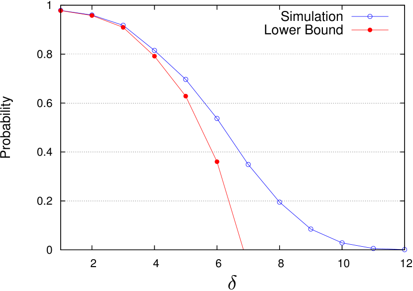
Figure 1: Sparse case: accumulate distribution of the minimum cut capacity $Pr[\lambda(G)\geq\delta]$ $(k=100,n=400)$: estimation by simulations and lower bounds

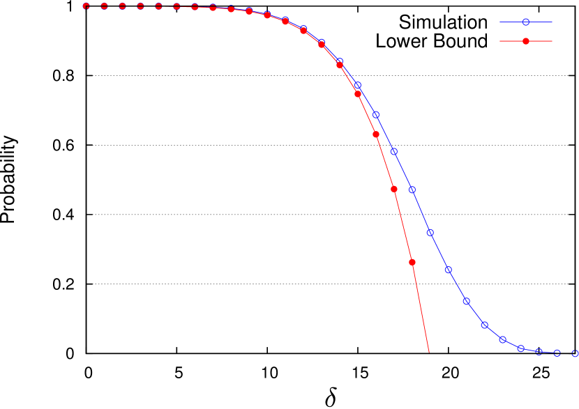
Figure 2: Dense case: accumulate distribution of the minimum cut capacity $Pr[\lambda(G)\geq\delta]$ $(k=100,n=700)$ estimation by simulations and lower bounds

V Conclusion

In this paper, a lower bound on the accumulate distribution of the minimum cut capacity for a random graph ensemble is presented. From the compute experiments, it is observed that the lower bound reflects actual statistical behavior of the minimum cut capacity. The bound and the proof technique presented in the paper would deepen our understanding on typical behaviors of the minimum-cut capacity.

The proof technique used here has close relationship to the analysis for the average weight distributions of LDGM codes with column weight 2. The one-to-one correspondence between a cut space and the row space of an incidence matrix implies that the minimum cut capacity is an analog of the minimum distance of the binary linear code defined by an incidence matrix. The analysis presented here has similarity to the typical minimum distance analysis of LDPC code ensembles [17].

An advantage of the proposed technique is its applicability for a graph ensemble with finite number of vertices and edges. Most related studies deal with asymptotic behaviors and cannot directly be applied to a finite size graph ensemble. Of course, it would be interesting to investigate the asymptotic behavior of the proposed lower bound when $n$ and $k$ approach infinity while maintaining the relationship $n=f(k)$ ($f$ is a real-valued function, e.g., $n=\beta k^{2}$).

The second advantage of the proposed technique is extensibility. In this paper, we discussed a simple graph ensemble, which is closely related to the Erdős-Rényi random graph ensemble [4]. The analysis for deriving the average cut-set weight distribution is approximately equivalent to the analysis of the average weight distribution of an LDGM code ensemble [6] or of the average coset weight distribution of an LDPC code ensemble [8]. Extension to other graph ensembles, such as regular or irregular bipartite graph ensembles, may be straightforward.

Acknowledgement

This work was partly supported by the Ministry of Education, Science, Sports and Culture, Japan, Grant-in-Aid, No. 22560370.

References

• [1] N. Alon and J.H. Spencer, β€œThe probabilistic method,” Wiley InterScience (2000).
• [2] B. Bollobas, β€œRandom graph, ” (2nd ed.) Cambridge University Press, 2001.
• [3] R. Diestel, β€œGraph theory, ” Springer-Verlag, New York, 2000.
• [4] P. ErdΕ‘s and A. RΓ©nyi, β€œOn random graphs I,” Publicationes Mathematicae, 6, pp.290-297, 1959.
• [5] S. L. Hakimi and H. Frank,β€œCut-set matrices and linear codes,” IEEE Trans. Inform.Theory, vol.IT-11, pp.457-458, July 1965.
• [6] C. H. Hsu and A. Anastasopoulos, β€œCapacity-achieving codes with bounded graphical complexity and maximum likelihood decoding,” IEEE Trans. Inform. Theory, pp.992-1006, vol.56, no. 3, Mar. 2010.
• [7] S.Litsyn and V. Shevelev, β€œOn ensembles of low-density parity-check codes: asymptotic distance distributions,” IEEE Trans. Inform. Theory, vol.48, pp.887–908, Apr. 2002.
• [8] T. Wadayama, β€œAverage coset weight distribution of combined LDPC matrix ensembles,” IEEE Trans. Inform. Theory, pp.4856- 4866, vol.52, no.11, Nov 2006.
• [9] T. Wadayama, β€œOn undetected error probability of binary matrix ensembles,” IEEE Trans. Inform. Theory, pp.2168-2176, vol.56, no. 5, May 2010.
• [10] H. Wang, P. Fan, K. B. Letaief, β€œMaximum flow and network capacity of network coding for ad-hoc networks, ” IEEE Trans. Wireless Comm., pp. 4193–4198, vol. 6, no.12, Dec. 2007.
• [11] D. R. Karger, β€œRandom sampling in cut, flow, and network design problems, ” Mathematics of Operations Research, vol. 24, no.2, pp.383–413, May 1999.
• [12] A. Ramamoorthy, J. Shi, R. D. Wesel, β€œOn the Capacity of network coding for random networks,” IEEE Trans. Inform. Theory, pp. 2878–2885, vol. 51, no.8, Aug. 2005.
• [13] A. Yano and T. Wadayama, β€œProbabilistic analysis of the network reliability problem on a random graph ensemble, ” arXiv:1105.5903, 2011.
• [14] T. Richardson and R. Urbanke, β€œModern coding theory,” Cambridge University Press, 2008.
• [15] A. Schrijver, β€œCombinatorial optimization, polyhedra and efficiency,” Springer-Verlag Berlin, 2003.
• [16] R. Ahlswede, N.Cai, S.Li, and R.Yeung, β€œNetwork information flow, ” IEEE Trans. on Inform. Theory, vol.46, pp.1204–1216, Apr. 2000
• [17] R.G.Gallager, β€œLow density parity check codes, ” MIT Press 1963.