Smooth Convergence away from Singular Sets

Abstract.

We consider sequences of metrics, $g_{j}$, on a compact Riemannian manifold, $M$, which converge smoothly on compact sets away from a singular set $S\subset M$, to a metric, $g_{\infty}$, on $M\setminus S$. We prove theorems which describe when $M_{j}=(M,g_{j})$ converge in the Gromov-Hausdorff sense to the metric completion, $(M_{\infty},d_{\infty})$, of $(M\setminus S,g_{\infty})$. To obtain these theorems, we study the intrinsic flat limits of the sequences. A new method, we call hemispherical embedding, is applied to obtain explicit estimates on the Gromov-Hausdorff and Intrinsic Flat distances between Riemannian manifolds with diffeomorphic subdomains.

Seven years after the publication of this paper in CAG, Brian Allen discovered a counter example to the published statement of Theorem 1.3. Note that Theorem 4.6 (which is the key theorem cited in other papers) remains correct. We have added an hypothesis to correct the statement of Theorem 1.3 and its consequences. This v4 includes corrections in blue, an erratum at the end of the introduction, and Brian Allen’s example in an appendix. An erratum is also being sent to the journal.

1. Introduction

The purpose of this paper is to provide general results concerning the limits of Riemannian manifolds which converge smoothly away from a singular set as follows:

Definition 1.1.

We will say that a sequence of Riemannian metrics, $g_{j}$, on a compact manifold, $M$, converges smoothly away from $S\subset M$ to a Riemannian metric $g_{\infty}$ on $M\setminus S$ if for every compact set $K\subset M\setminus S$, $g_{j}$ converge $C^{k,\alpha}$ smoothly to $g_{\infty}$ as tensors. In addition we say that it converges uniformly from below if there exists $\delta_{j}\to 0$ such that $g_{j}\geq(1-\delta_{j})^{2}g_{\infty}$ on $M\setminus S$.

The techniques developed in this paper will also be applied to other notions of smooth convergence away from singular sets in upcoming work of the first author, particular notions in which the sequence of manifolds need not be diffeomorphic. With any notion of smooth convergence away from a singular set, one must keep in mind that even when the singular set is an isolated point, smooth convergence away from that point does not even imply that $(M_{\infty},g_{\infty})$ is compact [Example 3.12]. Increasingly large distances may exist outside the compact sets used to define the smooth convergence.

Given two compact Riemannian manifolds, $M_{i}$, the Gromov-Hausdorff distance, $d_{GH}(M_{1},M_{2})$, is an isometry invariant. Introduced by Gromov in [Gro99], it is a distance on compact metric spaces in the sense that $d_{GH}(M_{1},M_{2})=0$ iff $M_{1}$ is isometric to $M_{2}$. When studying precompact domains within manifolds, one always takes the metric completion before examining the region using the Gromov-Hausdorff distance. Section 2 (see Definition 2.5).

Smooth limits away from singular sets, depend on the charts and tensors $g_{j}$ used to define the smooth limit (c.f. Example 3.7). Thus it is important to understand when the metric completion, $\bar{Y}$, of a smooth limit, $Y=(M\setminus S,g_{\infty})$, is in fact actually the Gromov-Hausdorff limit, $(M_{0},d_{0})$, of the original sequence of manifolds, $(M_{j},d_{j})$, where $d_{j}$ is the Riemannian distance defined by the Riemannian metric $g_{j}$.. Observe that these spaces need not be isometric (c.f. Example 3.1) and that the original sequence of manifolds might not even have a Gromov-Hausdorff limit (c.f. Example 3.11). If $M\setminus S$ is not connected there isn’t even a notion of the metric completion as a single metric space (c.f. Example 3.4).

Theorems relating Gromov-Hausdorff limits and smooth limits away from singular sets appear in work of Anderson, Bando-Kasue-Nakajima, Eyssidieux-Guedj-Zeriahi, Huang, Ruan-Zhong, Sesum, Tian and Tosatti particularly in the setting of Kahler Einstein manifolds [And89] [BKN89] [EGZ09] [Hua09] [RZ11] [Ses04] [Tia90] [Tos09]. However, even in this setting, the relationship is not completely clear and the limits need not agree [Ban90].

In this paper, our primary goal is to examine when the metric completion, $(M_{\infty},d_{\infty})$, of the smooth limit, $(M\setminus S,g_{\infty})$, is isometric to the Gromov-Hausdorff limit, $(M_{0},d_{0})$, of the original sequence of Riemannian manifolds $(M,g_{j})$. We prove a number of theorems and present a number of examples considering manifolds with and without Ricci curvature bounds. Perhaps the most important result is the following:

Theorem 1.2.

Let $M_{i}=(M,g_{i})$ be a sequence of oriented compact Riemannian manifolds with uniform lower Ricci curvature bounds,

(1.1) $$\rm{Ricci}_{g_{i}}(V,V)\geq(n-1)H\,g_{i}(V,V)\qquad\forall V\in TM_{i}$$

which converges smoothly away from $S$ uniformly from below where $S$ is a submanifold of codimension $2$.

If there is a connected precompact exhaustion, $W_{j}$, of $M\setminus S$,

(1.2) $$\bar{W}_{j}\subset W_{j+1}\textrm{ with }\bigcup_{j=1}^{\infty}W_{j}=M\setminus S$$

satisfying

(1.3) $$\operatorname{diam}(M_{i})\leq D_{0},$$

(1.4) $$\operatorname{Vol}_{g_{i}}(\partial W_{j})\leq A_{0},$$

and

(1.5) $$\operatorname{Vol}_{g_{i}}(M\setminus W_{j})\leq V_{j}\textrm{ where }\lim_{j\to\infty}V_{j}=0,$$

then

(1.6) $$\lim_{j\to\infty}d_{GH}(M_{j},N)=0,$$

where $N$ is the metric completion of $(M\setminus S,g_{\infty})$.

Note that, unlike prior existing results concerning the Gromov-Hausdorff limits of manifolds, here we require only area and volume controls on the connected precompact exhaustion. Theorem 1.2 is a consequence of Theorem 6.10, stated within, which assumes only that the connected precompact exhaustion is uniformly well embedded in the sense of Definition 5.1 . The necessity of the various hypothesis of these theorems is described in Remark 6.13. In particular the diameter hypothesis is unnecessary when the Ricci curvature is nonnegative.

The Ricci curvature condition in these theorems may be replaced by a requirement that the sequence of manifolds have a uniform linear contractibility function. See Definition 6.1, Theorem 6.7 and Theorem 6.6, stated within. The necessity of the various hypothesis of these theorems is described in Remark 6.8.

Observe our main theorems concern sequences of manifolds converging smoothly away from a singular set satisfying (1.4) and (1.5). In order to control the limits of such manifolds using only conditions on volumes, we apply techniques developed by the second author with Stefan Wenger in [SW10] and [SW11]. In attempt to keep this article self contained, we review convergence of Riemannian manifolds in Section 2. We provide extensive examples in Section 3. All examples are proven in detail with short statements for easy reference.

Our theorems are proven by studying the intrinsic flat limit of the manifolds [Definition 2.20]. This intrinsic flat distance, $d_{\mathcal{F}}(M_{1},M_{2})$ was originally defined in work of the second author with Wenger [SW11]. It is estimated by explicitly constructing a filling manifold, $B^{m+1}$, between the two given manifolds, finding the excess boundary manifold $A^{m}$ satisfying (2.11) and summing their volumes as in (2.12). See Remark 2.8 for a straight forward construction. Since $d_{\mathcal{F}}$ depends only on the Riemannian manifolds, $M_{i}$, as oriented metric spaces with a notion of integration over $m$ forms, we take settled completions rather than metric completions of open domains when analyzing the intrinsic flat distance (see Definition 2.9). If two completely settled oriented Riemannian manifolds, $M_{1}$ and $M_{2}$ have $d_{\mathcal{F}}(M_{1},M_{2})=0$ then there is an orientation preserving isometry between them [SW11]. See Section 2 for a review of the intrinsic flat distance and related concepts.

In Section 4 we prove new explicit estimates on the Gromov-Hausdorff, intrinsic flat and scalable intrinsic flat distances between pairs of manifolds which are diffeomorphic on subdomains [Theorem 4.6]. The subdomains need not be connected. These estimates are found by isometrically embedding the regions into a common metric space defined using a hemispherical construction [Proposition 4.2] and then measuring the Hausdorff, flat and scalable flat distances between their images respectively [Lemma 4.5]. Note that the Hausdorff distance measures distances between the images using tubular neighborhoods while the flat distance measures a filling volume between the images. These estimates have been applied in work of the second author with Dan Lee on questions concerning the Riemannian Penrose Inequality [LS11b] and in the first author’s doctoral dissertation [Lak13].

In Section 5, we prove theorems concerning the intrinsic flat limits of manifolds which converge smoothly away from singular sets. In particular, we prove:

Theorem 1.3.

Let $M_{i}=(M,g_{i})$ be a sequence of compact oriented Riemannian manifolds such that there is a submanifold, $S$, of codimension 2, and connected precompact exhaustion, $W_{j}$, of $M\setminus S$ satisfying (1.2) with $g_{i}$ converge smoothly to $g_{\infty}$ on $M\setminus S$ uniformly from below such that

(1.7) $$\operatorname{diam}_{M_{i}}(W_{j})\leq D_{0}\qquad\forall i\geq j,$$

(1.8) $$\operatorname{Vol}_{g_{i}}(\partial W_{j})\leq A_{0},$$

and

(1.9) $$\operatorname{Vol}_{g_{i}}(M\setminus W_{j})\leq V_{j}\textrm{ where }\lim_{j\to\infty}V_{j}=0.$$

Then

(1.10) $$\lim_{j\to\infty}d_{\mathcal{F}}(M_{j}^{\prime},N^{\prime})=0.$$

where $N^{\prime}$ is the settled completion of $(M\setminus S,g_{\infty})$.

This theorem is a consequence of Theorem 5.2 which assumes only that the connected precompact exhaustion is uniformly well embedded in the sense of Definition 5.1. We discuss the necessities of the conditions for these theorems in Remark 5.3. A key step in the proof is a technical proposition concerning the convergence of exhaustions of manifolds [Proposition 5.4].

In Section 6, we apply the theorems regarding intrinsic flat limits to prove the theorems concerning Gromov-Hausdorff limits mentioned earlier. Note that the second author and Stefan Wenger have proven that the intrinsic flat and Gromov-Hausdorff limits of sequences of manifolds agree when the sequence has nonnegative Ricci curvature and the volume is bounded below uniformly [SW10]. These results are reviewed in Section 6. Theorem 1.3 then immediately implies Theorem 6.6 and Theorem 1.2 when $H=0$. To obtain Theorem 1.2 for arbitrary values of $H$, we prove Proposition 6.12.

Applications of these results appear in joint work of the second author and Dan Lee concerning asymptotically flat rotationally symmetric Riemannian manifolds with positive scalar curvature that satisfy an almost equality in the Penrose inequality [LS11b]. We believe these results may also be applicable to open questions stated in [LS11a]. The first author is examining further applications in his doctoral dissertation.

The authors would like to thank the Simons Center for Geometry and Physics for its hospitality. Attending the many interesting talks there made it clear that a paper clarifying the applications of the intrinsic flat convergence to understand smooth limits away from singular sets would be useful to mathematicians in a wide variety of subfields of geometric analysis. We would also like to thank Xiaochun Rong for suggesting an important counter example and the referee for providing thorough and detailed suggestions that improved this paper throughout.

Errata:

Seven years after this paper was published in CAG, Brian Allen found a counter example to Theorem 1.3 which we present in the appendix. Theorem 1.3 is false as stated in the original publication for smooth convergence $g_{j}\to g_{\infty}$ on $M\setminus S$ where the converge is only uniform on compact sets $K\subset M\setminus S$. This theorem and its consequences Theorem 1.2 and Theorem 6.6 are easily corrected by adding in the assumption that the convergence of $g_{j}\to g_{\infty}$ is also uniform from below on $M\setminus S$.

The original error was traced by Brian Allen to a reversal of indices in limits in the original proof of Theorem 5.2. We find that by correcting the order of the limits in Definition 5.1 of uniform well embeddedness, we can prove Theorem 5.2 as originally stated. We also correct the proof Lemma 5.7 to adapt to this new definition of uniform well embeddedness using the notion of smooth convergence away from a singular set uniformly from below. Thus Theorem 1.3 and its consequences (Theorem 1.2 and Theorem 6.6) are true assuming this stronger hypothesis. These corrections are made in blue within this v4 of the paper.

This paper has been cited many times since its publication. We believe the only paper that needs revision is [Lak12] by the first author of this paper. The other papers apply only Theorem 4.6, which remains correct as originally stated and proven.

2. Background

All notions of distances between Riemannian manifolds studied in this paper are built upon Gromov’s idea that one may view Riemannian manifolds as metric spaces and isometrically embed them into a common metric space. In this paper, a key part of our work relies on constructing such isometric embeddings. We review Gromov’s key ideas in Subsection 2.1.

To estimate the Gromov-Hausdorff distance between a pair of Riemannian manifolds, one needs only find a pair of isometric embeddings $\varphi_{i}:M^{m}_{i}\to Z$ into a common complete metric space $Z$ and then measure the Hausdorff distances between the images. We review the definition of the Hausdorff and Gromov-Hausdorff in Subsection 2.2.

To estimate the intrinsic flat distance one must measure the flat distance between these images. So one may construct a Riemannian manifold of one dimension higher filling in the space between the two images, possible with some excess boundary. Note that one can only measure the intrinsic flat distance between oriented manifolds with finite volume of the same dimension. See Subsection 2.3.

The scalable intrinsic flat distance is also defined using filling manifolds and excess boundaries. It is reviewed in Subsection 2.4.

Remarks 2.3,  2.6,  2.8 and 2.11 capture the key properties of these three notions of distance needed to estimate them for the purposes of this paper.

2.1. Metric Spaces and Isometric Embeddings

Definition 2.1.

Recall that one may view a Riemannian manifold $(M,g)$ as a metric space $(M,d)$ by defining the distances between points as follows:

(2.1) $$d(x_{1},x_{2})=\inf\left\{L_{g}(\gamma):\,\gamma(0)=x_{1},\,\gamma(1)=x_{2}\right\}$$

where

(2.2) $$L_{g}(\gamma)=\int_{0}^{1}g(\gamma^{\prime}(t),\gamma^{\prime}(t))^{1/2}dt$$

Given a connected subdomain, $W\subset M$, and $x,y\in W$, the ”restricted metric”, $d_{M}(x,y)$, will denote the distance between $x$ and $y$ measured as in (2.1) where the infimum taken over all curves $\gamma:[0,1]\to M$, while the ”induced length metric”, $d_{W}(x,y)\geq d_{M}(x,y)$, has the infimum taken only over curves $\gamma:[0,1]\to W$. We denote the restricted and intrinsic length diameters of $U\subset W\subset M$ as follows

(2.3) $$\operatorname{diam}_{M}(U) = \sup\{d_{M}(x,y):\,x,y\in U\}$$

(2.4) $$\operatorname{diam}_{W}(U) = \sup\{d_{W}(x,y):\,x,y\in U\}$$

More generally a length metric space is a metric space whose distances are defined as an infimum of lengths of rectifiable curves. Compact length metric spaces always have minimizing geodesics between points achieving the distance.

In this paper we will often define metric spaces, $Z$, by gluing together Riemannian manifolds with corners along their boundaries. In this way we may still apply (2.1) to define the distances between points. Again, for connected subdomains, $W\subset Z$, one has both an induced length metric, $d_{W}$, and a restricted distance $d_{Z}\leq d_{W}$ just as in Definition 2.1.

Definition 2.2.

An isometric embedding $\varphi:X\to Z$ is a distance preserving map

(2.5) $$d_{Z}(\varphi(x_{1}),\varphi(x_{2}))=d_{X}(x_{1},x_{2})\qquad\forall x_{1},x_{2}\in X$$

One should be aware that a Riemannian isometric embedding defined by the fact that $d\varphi$ is an isometry on the tangent spaces at each point, is not necessarily an isometric embedding. For example, the natural embedding of the sphere into Euclidean space is not an isometric embedding with the standard metric on the sphere. See Figure 1.

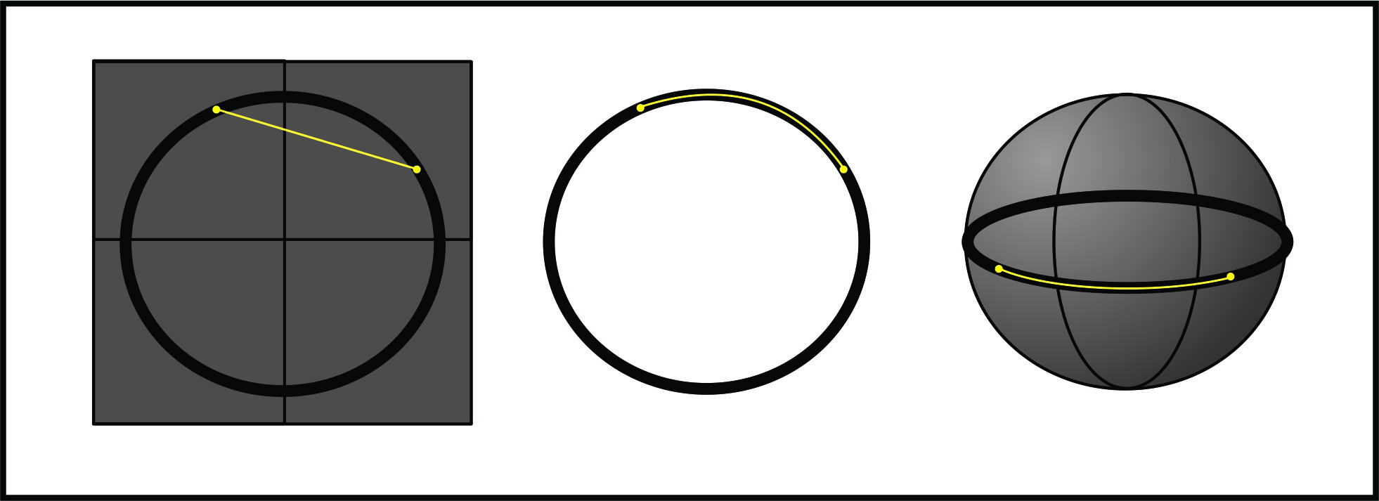
Figure 1. $S^{1}$ in the center isometrically embeds into $S^{2}$ on the right, but does not isometrically embed into $\mathbb{E}^{2}$ on the left.

Remark 2.3.

Suppose two manifolds, $M_{i}$ have diffeomorphic subdomains, $U_{i}$, then a filling manifold can be constructed of the form $U\times[h_{1},h_{2}]$ with a well chosen metric $g^{\prime}$ so that $M_{i}$ isometrically embed into

(2.6) $$Z=M_{1}\sqcup(U\times[h_{1},h_{2}])\sqcup M_{2}.$$

Here $Z$ is glued together so that $U_{i}$ is identified point to point with $U\times\{h_{i}\}$. A precise way of choosing such a $g^{\prime}$ will be given in Theorem 4.6. See Figure 2.

2.2. The Gromov-Hausdorff Distance

The Gromov-Hausdorff distance between a pair of Riemannian manifolds is estimated by taking isometric embeddings into a common metric space $Z$ and measuring the Hausdorff distance between them. This distance was introduced by Gromov in [Gro99]. It is defined on pairs of metric spaces.

Definition 2.4 (Hausdorff).

Given two subsets $Y_{1},Y_{2}\subset Z$, the Hausdorff distance is defined

(2.7) $$d_{H}^{Z}(Y_{1},Y_{2})=\inf\left\{r:\,Y_{1}\subset T_{r}(Y_{2})\textrm{ and }Y_{2}\subset T_{r}(Y_{1})\right\}$$

where $T_{r}(Y)=\left\{z\in Z:\,\exists y\in Y\,s.t.\,d(y,z)<r\right\}$.

One may immediately observe that the topology and dimension of subsets which are close in the Hausdorff sense can be quite different.

Definition 2.5 (Gromov).

Given a pair of metric spaces $(X_{1},d_{1})$ and $(X_{2},d_{2})$, the Gromov-Hausdorff distance between them is

(2.8) $$d_{GH}(X_{1},X_{2})=\inf\left\{d^{Z}_{H}(\varphi_{1}(X_{1}),\varphi_{2}(X_{2})):\,\,\varphi_{i}:X_{i}\to Z\right\}$$

where the infimum is taken over all common metric spaces, $Z$, and all isometric embeddings, $\varphi_{i}:X_{i}\to Z$.

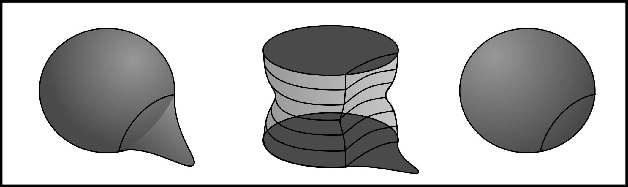
Figure 2. $M_{1}$ and $M_{2}$ depicted on the left and the right isometrically embed into $Z$ in the center. See Remarks 2.3 and 2.6.

Remark 2.6.

In Figure 2 depicting Remark 2.3, we see that

(2.9) $$d_{GH}(M_{1},M_{2})\leq d_{H}^{Z}(\varphi_{1}(M_{1}),\varphi_{2}(M_{2}))$$

which is roughly the length of a curve from the tip of the bump in $M_{1}$ running back within $\varphi(M_{1})\subset Z$ to the warped region $U\times[h_{1},h_{2}]$ and then straight up to $M_{2}$. Later in this paper Theorem 4.6 we will find a precise description of the metric on the metric space $Z$ of Figure 2.

Gromov proved in [Gro99] that this a distance between compact metric spaces, in the sense that $d_{GH}(X_{1},X_{2})=0$ iff $X_{1}$ and $X_{2}$ are isometric. In general one takes the metric completion, $\bar{X}$, of a precompact space, $X$, before discussing it’s Gromov-Hausdorff distance and we will do the same here. Recall that the metric completion is defined as follows:

Definition 2.7.

Given a precompact metric space, $X$, the metric completion, $\bar{X}$ of $X$ is the space of Cauchy sequences, $\{x_{j}\}$, in $X$ with the metric

(2.10) $$d(\{x_{j}\},\{y_{j}\})=\lim_{j\to\infty}d_{X}(x_{j},y_{j})$$

and where two Cauchy sequences are identified if the distance between them is $0$. There is an isometric embedding, $\varphi:X\to\bar{X}$, defined by $\varphi(x)=\{x\}$ where $\{x\}$ is a constant sequence. Lipschitz functions, $F:X\to Y$, extend to $F:\bar{X}\to Y$ via $F(\{x_{j}\})=\lim_{j\to\infty}F(x_{j})$ as long as $Y$ is complete.

Gromov’s compactness theorem states that a sequence of Riemannian manifolds $M_{j}^{m}$ with a uniform lower bound on Ricci curvature have a subsequence which converges in the Gromov-Hausdorff sense. More generally one may replace the Ricci curvature bound with a bound on the number, $N(r)$, of disjoint balls of radius, $r$, that can be placed in a metric space, $X$. That is, a sequence of metric spaces $X_{j}$ with a uniform bound on $N(r)$ for all $r$ sufficiently small, has a subsequence which converges in the Gromov-Hausdorff sense to a compact limit space $X$. Conversely, if $d_{GH}(X_{j},X)\to 0$, then there is a uniform bound on $N(r)$. [Gro99].

2.3. The Intrinsic Flat Distance

To estimate the intrinsic flat distance between a pair of oriented Riemannian manifolds one again needs only find a pair of isometric embeddings, $\varphi_{i}:M^{m}_{i}\to Z$, into a common complete metric space, $Z$. When one finds a filling submanifold, $B^{m+1}\subset Z,$ and an excess boundary submanifold, $A^{m}\subset Z$, such that

(2.11) $$\int_{\varphi_{1}(M_{1})}\omega-\int_{\varphi_{2}(M_{2})}\omega=\int_{B}d\omega+\int_{A}\omega,$$

then the intrinsic flat distance is bounded by

(2.12) $$d_{\mathcal{F}}(M^{m}_{1},M^{m}_{2})\leq\operatorname{Vol}_{m}(A^{m})+\operatorname{Vol}_{m+1}(B^{m+1}).$$

Generally the filling manifold and excess boundary can have corners and more than one connected component. See Figure 7.

Remark 2.8.

In Figure 2 depicting Remark 2.3, we have $M_{i}$ isometrically embedded into a well chosen metric space

(2.13) $$Z=M_{1}\sqcup(U\times[h_{1},h_{2}])\sqcup M_{2}.$$

Applying (2.11) to

(2.14) $$B=U\times[h_{1},h_{2}]$$

we see that the excess boundary

(2.15) $$A=(M_{1}\setminus U_{1})\cup(\partial U\times[h_{1},h_{2}])\cup(M_{2}\setminus U_{2}).$$

Then

$$d_{\mathcal{F}}(M_{1},M_{2}) \leq \operatorname{Vol}_{m}(M_{1}\setminus U_{1})+\operatorname{Vol}_{m}(M_{2}\setminus U_{2})+\operatorname{Vol}_{m}(\partial U\times[h_{1},h_{2}])$$

$$+ \operatorname{Vol}_{m+1}(U\times[h_{1},h_{2}],g^{\prime}).$$

An explicit construction of the metric $g^{\prime}$ on $U\times[h_{1},h_{2}]$ in Theorem 4.6, allows one to precisely estimate the volume of $U\times[h_{1},h_{2}]$ and $\partial U\times[h_{1},h_{2}]$.

To understand limits of sequences of Riemannian manifolds, the intrinsic flat distance was defined on a larger class of metric spaces called integral current spaces in [SW11]. An integral current space, $(X,d,T)$, is a metric space, $X$, with a metric, $d$, and an integral current structure, $T$, such that $\rm{set}(T)=X$. An oriented Riemannian manifold, $(M,g)$, of finite volume, has a metric, $d_{M}$, defined as in Definition 2.1 and an integral current structure, $T$, acting on $m$ dimensional differential forms, $\omega$ as

(2.16) $$T(\omega)=\int_{M}\omega.$$

More generally, the integral current structure, $T$, of an integral current space, $(X,d,T)$, is an $m$ dimensional integral current $T\in{\mathbf{I}}_{m}(\bar{X})$ defined as in Ambrosio-Kirchheim’s work [AK00]. The integral current structure $T$ provides both an orientation and a measure called the mass measure denoted $||T||$ and $\rm{set}(T)$ is the set of positive lower density for this measure. On a oriented Riemannian manifold, the mass measure is just the Lebesgue measure. More generally the mass measure can have integer valued weights.

If $(M^{m},g)$ is a Riemannian manifold with singularities on a subset $S$ such that the Hausdorff measure, $\mathcal{H}_{m}(S)=0$, then one obtains a corresponding integral current space by taking the settled completion of $M\setminus S$ defined as follows:

Definition 2.9.

[SW11] The settled completion, $X^{\prime}$, of a metric space $X$ with a measure $\mu$ is the collection of points $p$ in the metric completion $\bar{X}$ which have positive lower density:

(2.17) $$\liminf_{r\to 0}\mu(B_{p}(r))/r^{m}>0.$$

The resulting space is then ”completely settled”.

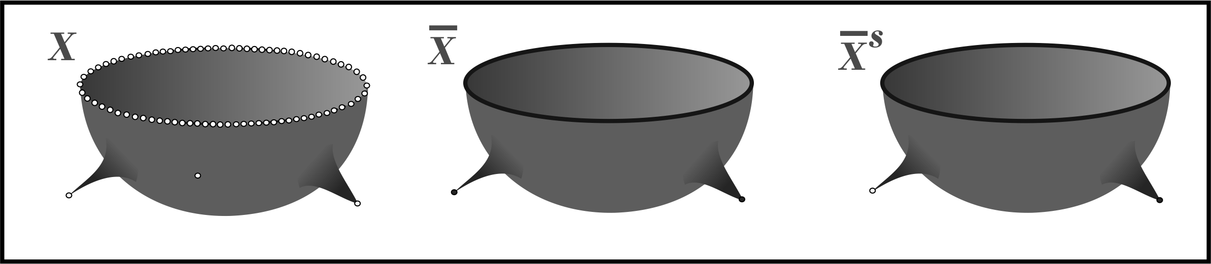
Figure 3. The completion, $\bar{X}$ includes the boundary and fills in the three ”holes” and the settled completion, $X^{\prime}$, removes the cusped singularity but keeps the boundary, cone tip and smoothly filled hole.

If a manifold has only point singularities, one includes all conical tips and does not include cusp tips in a manifold with point singularities. See Figure 3. This is natural because the essential property of an integral current space is its integration and points of $0$ lower density do not contribute to that integration. In fact integral current spaces are completely settled with respect to the mass measure, $||T||$, as a consequence of the requirement that $\rm{set}(T)=X$.

The mass of an integral current space, ${\mathbf{M}}(T)$, is a weighted volume of sorts which takes into account the integer valued Borel weight defining the current structure on the space. When the integral current space is an oriented Riemannian manifold then its mass is just its volume, ${\mathbf{M}}(M)=\operatorname{Vol}(M)$.

The boundary of an integral current space is defined

(2.18) $$\partial(X,d,T)=(\rm{set}(\partial T),d,\partial T)$$

where $\partial T$ is the boundary of the integral current defined as in [AK00] so that it satisfies Stoke’s Theorem. When $M$ is a Riemannian manifold, its boundary is just the usual boundary, $\partial M$.

The flat distance between two integral currents is defined as in [FF60]

(2.19) $$d_{{F}}(T_{1},T_{2})=\inf\left\{{\mathbf{M}}(B^{m+1})+{\mathbf{M}}(A^{m}):\,T_{1}-T_{2}=A+\partial B\right\}.$$

That is $T_{1}(\omega)-T_{2}(\omega)=A(\omega)+\partial B(\omega)=A(\omega)+B(d\omega)$.

Definition 2.10 (Sormani-Wenger).

The intrinsic flat distance between integral current spaces is defined in [SW11] as

(2.20) $$d_{\mathcal{F}}\big{(}(X_{1},d_{1},T_{1}),(X_{2},d_{2},T_{2})\big{)}=\inf\left\{d^{Z}_{F}(\varphi_{1\#}T_{1},\varphi_{2\#}T_{2});\,\varphi_{i}:X_{i}\to Z\right\}$$

where the infimum is taken over all common complete metric spaces, $Z$, and all isometric embeddings $\varphi_{i}:X_{i}\to Z$ and where $\varphi_{\#}$ is the push forward map on integral currents.

If one constructs a specific $Z$ and isometric embeddings $\varphi_{i}:M_{i}\to Z$, then one needs only estimate the flat distance between the images to obtain an upper bound for the infimum in (2.20). An explicit filling manifold $B$ satisfying (2.11), then provides an upper bound on the infimum in (2.19). This is how one obtains the estimate in (2.12). See also Remark 2.8.

In [SW11] it is proven that this is a distance between precompact integral current spaces in the sense that $d_{\mathcal{F}}\big{(}(X_{1},d_{1},T_{1}),(X_{2},d_{2},T_{2})\big{)}=0$ iff there is a current preserving isometry from $X_{1}$ to $X_{2}$. When the integral current spaces are oriented manifolds, then there is an orientation preserving isometry.

Note that all integral current spaces are metric spaces but they need not be length spaces. As will be seen in Example 3.4 a sequence of connected Riemannian manifolds may converge in the intrinsic flat sense to an integral current space which has broken apart due to the development of a cusp singularity. So the limit is not a length metric space.

In [SW11] it is proven that if $(M,g_{j})$ converge smoothly to $(M,g_{\infty})$ then they converge in the intrinsic flat sense. In fact, precise estimates on the intrinsic flat distance are given in terms of the Lipschitz distance, the diameters and the volumes of the spaces. The bounds are found using geometric measure theory. Here we provide a new estimate relating the intrinsic flat and Lipschitz distances by explicitly constructing a filling manifold between them [Lemma 4.5].

If a sequence of oriented Riemannian manifolds with a uniform upper bound on their volumes and volumes of their boundaries converges in the Gromov-Hausdorff sense to a compact metric space $(Y,d)$, then a subsequence converges in the intrinsic flat sense to $(X,d,T)$ where $X\subset Y$ and the metric $d$ is restricted from $Y$ [SW11] [Thm 3.20]. In Example 3.4 we see that this may be a proper subset. In fact the Intrinsic flat limit may be the $(0,0,0)$ integral current space if $(Y,d)$ has a lower dimension than the manifolds in the sequence [SW11].

In [SW10] two theorems were proven indicating when the intrinsic flat limit and the Gromov-Hausdorff limits agree. These theorems will be reviewed later in the paper as they are applied. We will also apply the techniques in their proofs to prove Theorem 1.2.

2.4. The Scalable Intrinsic Flat Distance

The scalable intrinsic flat distance was suggested as a notion in work of the second author with Dan Lee [LS11a] following a recommendation of Lars Andersson. It is defined to scale with distance when the Riemannian manifolds are rescaled. In particular,

(2.21) $$d_{s\mathcal{F}}(M^{m}_{1},M^{m}_{2})\leq\left(\operatorname{Vol}_{m}(A^{m})\right)^{1/m}+\left(\operatorname{Vol}_{m+1}(B^{m+1})\right)^{1/(m+1)}$$

whenever there exist isometric embeddings, $\varphi_{i}:M^{m}_{i}\to Z$, into a common complete metric space, $Z$, and one finds a filling submanifold, $B^{m+1}\subset Z,$ and an excess boundary submanifold, $A^{m}\subset Z$, satisfying (2.11).

Remark 2.11.

In the setting of Remark 2.8 depicted in Figure 2 we see that

$$d_{s\mathcal{F}}(M_{1},M_{2}) \leq \operatorname{Vol}_{m+1}(U\times[0,h],g^{\prime})^{1/(m+1)}$$

$$+ \left(\operatorname{Vol}_{m}(M_{1}\setminus U_{1})+\operatorname{Vol}_{m}(M_{2}\setminus U_{2})+\operatorname{Vol}_{m}(\partial U\times[h_{1},h_{2}],g^{\prime})\right)^{1/m}.$$

More precisely:

Definition 2.12.

The scalable intrinsic flat distance between integral current spaces is defined as

(2.22) $$d_{s\mathcal{F}}((X_{1},d_{1},T_{1}),(X_{2},d_{2},T_{2}))=\inf\left\{d^{Z}_{sF}(\varphi_{1\#}T_{1},\varphi_{2\#}T_{2});\,\varphi_{i}:X_{i}\to Z\right\}$$

where the infimum is taken over all common complete metric spaces, $Z$, and all isometric embeddings $\varphi_{i}:X_{i}\to Z$ and where $\varphi_{\#}$ is the push forward map on integral currents and where the scalable flat distance between $m$ dimensional integral currents is defined by

(2.23) $$d_{sF}(T_{1},T_{2})=\inf\left\{{\mathbf{M}}(B)^{1/(m+1)}+{\mathbf{M}}(A)^{1/m}:T_{1}-T_{2}=A+\partial B\right\}$$

3. Examples

The examples in the section are all fine.

The following examples are presented to indicate how little control one may have on limits of manifolds which converge smoothly away from singular sets and to prove the necessity of the conditions in our theorems. The proofs of these examples will sometimes rely on our theorems proven below but we include them up front so that they can be kept in mind when reading the remainder of the paper.

3.1. Losing a Region

Example 3.1.

There are metrics, $g_{j}$, on the sphere, $M^{3}$, such that $(M^{3},g_{j})$ converge smoothly away from $S=\bar{B}_{p_{0}}(\pi/16)$, such that the metric completion of the smooth limit away from $S$ is $S^{3}\setminus B_{p_{0}}(\pi/16)$, the standard round sphere $(S^{3},g_{0})$ with a ball removed. The smooth limit of $M^{3}$ without the singular set removed is the entire round sphere and this agrees with the intrinsic flat and Gromov-Hausdorff limits (c.f. Lemma 4.5).

Proof.

Taking the metrics, $g_{j}=g_{0}$, we have a constant sequence of standard spheres. So the intrinsic flat and Gromov-Hausdorff limits are clearly the standard sphere. Furthermore $(g_{j},M\setminus S)$ clearly converges to $(g_{0},M\setminus\bar{B}_{p_{0}}(\pi/16))$ whose metric completion is $(g_{0},M\setminus{B}_{p_{0}}(\pi/16))$. ∎

3.2. Cones and Cusps

Example 3.2.

There are metrics $g_{j}$ on the sphere $M^{3}$ such that $(M^{3},g_{j})$ converge smoothly away from a point singularity $S=\{p_{0}\}$ and the metrics $g_{j}$ form a conical singularity at $p_{0}$. The Gromov-Hausdorff and intrinsic flat limits agree with the metric completion of $(M\setminus S,g_{\infty})$ which is the sphere including the conical tip.

Proof.

More precisely the metrics $g_{j}$ are defined by

(3.1) $$g_{j}=dr^{2}+f_{j}^{2}(r)g_{S^{2}}\textrm{ for }r\in[0,\pi]$$

where $f_{j}(r)=\left(1/j\right)\sin(r)+\left(1-1/j\right)f(r)$ in which, $f(r)$ is a smooth function such that:

(3.2) $$f(r)=\sin(r)\;\text{for}\;r\in[0,\pi/2],$$

and,

(3.3) $$f(r)=-\frac{2}{\pi}\left(r-\pi\right)\;\text{for}\;r\in[3\pi/4,\pi].$$

For any $\delta>0$, $f_{j}$ converge to $f$ smoothly on $[0,\pi-\delta]$. Thus $g_{j}$ converge smoothly on compact subsets of $M\setminus S$ to

(3.4) $$g_{\infty}=dr^{2}+f^{2}(r)g_{S^{2}}.$$

The metric completion of $(M\setminus S,g_{\infty})$ then adds in a single point $p_{0}$ at $r=\pi$. Since

(3.5) $$\liminf_{r\to 0}\mu(B_{p_{0}}(r))/r^{3}=\frac{4}{3\pi^{2}}vol(S^{2})=\frac{16}{3\pi}>0,$$

the point, $p_{0}$, is also included in the settled completion of $(M\setminus S,g_{\infty})$. To complete the proof of the claim we could apply Theorem 1.3. ∎

Example 3.3.

There are metrics $g_{j}$ on the sphere $M^{3}$ such that $(M^{3},g_{j})$ converge smoothly away from a point singularity $S=\{p_{0}\}$ and the metrics $g_{j}$ form a cusp singularity at $p_{0}$. The Gromov-Hausdorff agree with the metric completion of $(M\setminus S,g_{\infty})$ which is the sphere including the cusped tip. However the intrinsic flat limit of $(M\setminus S,g_{\infty})$ does not include the cusped tip because it has $0$ density. So the intrinsic flat limit is the settled completion of $(M\setminus S,g_{\infty})$ which in this case is $(M\setminus S,g_{\infty})$

Proof.

More precisely the metrics $g_{j}$ are defined by

(3.6) $$g_{j}=dr^{2}+f_{j}^{2}(r)g_{S^{2}}\textrm{ for }r\in[0,\pi]$$

where $f_{j}(r)=\left(1/j\right)\sin(r)+\left(1-1/j\right)f(r)$ in which, $f(r)$ is a smooth function such that:

(3.7) $$f(r)=\sin(r)\;\text{for}\;r\in[0,\pi/2],$$

and,

(3.8) $$f(r)=\frac{4}{\pi^{2}}\left(r-\pi\right)^{2}\;\text{for}\;r\in[3\pi/4,\pi].$$

For any $\delta>0$, $f_{j}$ converge to $f$ smoothly on $[0,\pi-\delta]$. Thus $g_{j}$ converge smoothly on compact subsets of $M\setminus S$ to

(3.9) $$g_{\infty}=dr^{2}+f^{2}(r)g_{S^{2}}.$$

The metric completion of $(M\setminus S,g_{\infty})$ then adds in a single point $p_{0}$ at $r=\pi$. Since

(3.10) $$\liminf_{r\to 0}\mu(B_{p_{0}}(r))/r^{3}=\liminf_{r\to 0}\frac{4}{5\pi^{2}}r^{2}vol(S^{2})=0,$$

the point, $p_{0}$, is not included in the settled completion of $(M\setminus S,g_{\infty})$.

This Gromov-Hausdorff and Intrinsic Flat limits in this example were proven to be as claimed in the Appendix of [SW11]. One may also apply Theorem 4.6 to reprove this. ∎

3.3. Not Connected

Example 3.4.

There are smooth metrics $g_{i}$ on the sphere, $M^{3}$, converging smoothly away from the equator, $S$, such that the equator pinches to $0$. Then $(M^{3}\setminus S,g_{i})$ has two components, each converging to a standard sphere with a point removed. The metric completion of each of the two disjoint metric spaces is a standard sphere. However the Gromov-Hausdorff limit is a pair of spheres joined at a point singularity. So we see why connectedness of $M^{3}\setminus S$ is a necessary condition in Theorem 5.2. Here the singular set is of codimension 1.

Remark 3.5.

In upcoming work of the first author [Lak13], appropriate gluings of disjoint metric spaces are taken to recover the Gromov-Hausdorff limit when $M\setminus S$ is not connected.

Proof.

Let $\phi(x)$ be a smooth bump function on $\mathbb{R}$ with the following properties:

(3.11) $$\int_{-\infty}^{\infty}\;\phi(x)\;dx=1$$

(3.12) $$\lim_{\epsilon\to 0}\phi_{\epsilon}(x)=\lim_{\epsilon\to 0}\epsilon^{-1}\phi(x/\epsilon)=\delta_{0}(x),$$

where $\delta_{0}(x)$ is the Dirac delta function at $0$. Let

(3.13) $$\Phi_{1/i}\left(|\sin(2x)|\right)(r)=\phi_{1/i}(x)*|\sin(2x)|(r)=\int_{-\infty}^{\infty}\;\phi_{1/i}(r-x)\;|\sin(2x)|\;\mathrm{d}x.$$

It is standard that the sequence is smooth and converges to $|\sin(2r)|$ as $i\to\infty$. Now, take a partition of unity $\{\psi,1-\psi\}$ on $[0,\pi]$ such that $\operatorname{supp}(\psi)\subset[\pi/8,7\pi/8]$ and $\psi=1$ on $[\pi/4,3\pi/4]$. We take the sequence of metrics

(3.14) $$g_{i}=dr^{2}+f_{i}^{2}(r)g_{S^{2}}$$

where,

(3.15) $$f_{i}(r)=\frac{1}{i}\sin(r)+\frac{i-1}{2i}\biggl{(}\left(1-\psi(r)\right)\left(|\sin(2r)|\right)+\psi(r)\;\Phi_{1/i}\left(|\sin(2x)|\right)(r)\biggr{)}$$

These are smooth metrics for $r\in[0,\pi]$ because $f_{i}(r)>0$ for $r\in(0,\pi)$,

(3.16) $$f_{i}^{\prime}(0)=\frac{1}{i}+\frac{2(i-1)}{2i}=1,$$

(3.17) $$f_{i}^{\prime}(\pi)=-\frac{1}{i}-\frac{2(i-1)}{2i}=-1$$

and $f_{i}^{\prime\prime}(0)=f_{i}^{\prime\prime}(\pi)=0.$ As $i\to\infty$, $g_{i}$ converge smoothly away from $r^{-1}(\pi/2)$ to

(3.18) $$g_{\infty}=dr^{2}+\frac{\sin^{2}(2r)}{4}g_{S^{2}}$$

which is a metric on a pair of spheres, each with a point removed. The metric completion keeps the pair of spheres disjoint, endowing each with its own point of completion.

The Gromov-Hausdorff and intrinsic flat limits however are a connected pair of spheres joined at point which creates a conical singularity. This can be seen because the distances $d_{i}$ defined on $M_{i}$ using $g_{i}$ are in fact converging in the Lipschitz sense to $d_{\infty}$ defined by using the infimum of lengths, $L_{\infty}$, of curves between points where

(3.19) $$L_{\infty}(C)=\int_{0}^{1}g_{\infty}(C^{\prime}(s),C^{\prime}(s))^{1/2}\,ds.$$

Taking $W_{j}=r^{-1}[0,\pi/2-1/j]\cup r^{-1}[\pi/2+1/j,\pi]$, then we have smooth convergence on $W_{j}$. The uniform embeddedness constants converge to $0$. Both $\operatorname{Vol}_{g_{i}}(V\setminus W_{j})<V_{j}$ with $V_{j}\to 0$ and $\operatorname{Vol}_{g_{i}}(\partial W_{j})\leq A_{j}$ with $A_{j}\to 0$. So we only fail the connectedness hypothesis of this theorem. ∎

3.4. Bubbling

Example 3.6.

There are smooth metric $g_{i}$ on the sphere, $M^{3}$ converging smoothly away from the singular set $S=\left\{p_{0}\right\}$ to a sphere. Yet $(M^{3},g_{i})$ converge in the Gromov-Hausdorff and intrinsic flat sense to a pair of spheres meeting at $p_{0}$. See Figure 4.

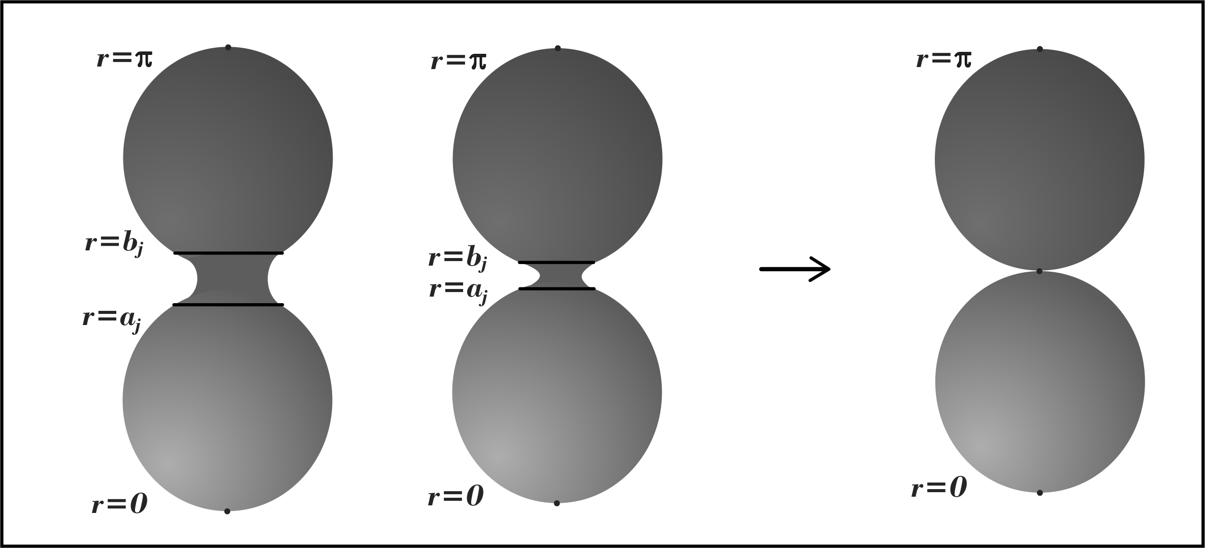
Figure 4. Example 3.6.

Proof.

Let

(3.20) $$g_{i}=h_{i}^{2}(r)dr^{2}+f_{i}^{2}(r)g_{S^{2}}$$

where

(3.21) $$h_{i}(r)=1 r\in[0,a_{i}]$$ on

(3.22) $$f_{i}(r)=\sin(r) r\in[0,a_{i}]$$ on

where $a_{i}=\pi-\pi/(10i)$ so that $g_{i}$ converges smoothly away from $S$ to the round metric $g_{\infty}$ on the sphere. The metric completion of $(M\setminus S,g_{\infty})$ is the round sphere.

Now we set

(3.23) $$h_{i}(r)=10i r\in[b_{i},\pi]$$ on

(3.24) $$f_{i}(r)=\sin((\pi-r)/(10i)) r\in[b_{i},\pi]$$ on

where $b_{i}=\pi-(\pi-\pi/(10i))/(10i)$ so there is symmetry and we extend them smoothly for $r\in[a_{i},b_{i}]$ so that

(3.25) $$h_{i}(a_{i})=1\leq h_{i}(r)\leq 10i=h_{i}(b_{i})$$

and

(3.26) $$0<f_{i}(r)<\max\{f_{i}(a_{i}),f_{i}(b_{i})\}.$$

These thin regions are converging to a single point. So the Gromov-Hausdorff limit of $(M,g_{i})$ is a pair of standard spheres joined at a point and the intrinsic flat limit is the same. The smooth limit away from $S$ missed the second sphere! ∎

3.5. Losing Volume in the Limit

Example 3.7.

There are $(M^{3},g_{i})$ all isometric to the standard sphere which converge smoothly away from a singular set $S=\{p_{0}\}$ to $(M\setminus S,g_{\infty})$ which is isometric to an open hemisphere. The metric completion agrees with the settled completion, $(M_{\infty},d_{\infty})$ which is isometric to a closed hemisphere. The singular set is codimension $2$ in $M$. This example satisfied all the conditions of all of our Theorems concerning smooth convergence away from singular sets except $\operatorname{Vol}(M\setminus W_{j})<V_{j}$ where $\lim_{j\to\infty}V_{j}=0$.

Proof.

Again we view $M^{3}=S^{3}$ as a warped product with a warping function $r\in[0,\pi]$, such that $r(p_{0})=\pi$. Let

(3.27) $$g_{i}=(h_{i}^{\prime}(r))^{2}dr^{2}+\sin^{2}(h_{i}(r))g_{S^{2}}$$

where $h_{i}(r)$ is a smooth increasing function such that

(3.28) $$h_{i}(r) = r(\pi/2)/(\pi-\pi/(2i))\textrm{ for }r\in[0,\pi-1/i]$$

(3.29) $$h_{i}(r) = \pi-(r-\pi)(1/(2i))(\pi-1/(2i))\textrm{ for }r\in[\pi-1/(2i),\pi].$$

Then the diffeomorphism which maps $r\mapsto s=h_{i}(r)$ is an isometry from $(M^{3},g_{i})$ to $(S^{3},g_{S^{3}})$.

On any compact set $K\subset M\setminus S$, there exists a $j$ sufficiently large that $K\subset r^{-1}[0,\pi-1/j]$. Taking $i\to\infty$ we see that on $K$, $h_{i}(r)\to r/2$ and $g_{i}$ converge smoothly to

(3.30) $$g_{\infty}=(1/2)^{2}dr^{2}+\sin^{2}(r/2)g_{S^{2}}.$$

Thus $(M\setminus S,g_{\infty})$ is isometric to an open hemisphere via the isometry which maps $r\mapsto s=r/2$. The metric completion is then the closed hemisphere and the settled completion agrees with the metric completion because every point in the closed hemisphere has positive lower density.

Setting $W_{j}=r^{-1}[0,\pi-1/j]$, we see that

(3.31) $$\operatorname{Vol}_{g_{i}}(\partial W_{j})\leq 4\pi.$$

Clearly the diameter, volume, Ricci curvature and contractibility conditions all hold because the sequence of $(M,g_{j})$ are all isometric to spheres. However

(3.32) $$\lim_{i\to\infty}\operatorname{Vol}_{g_{i}}(M\setminus W_{j})\geq\operatorname{Vol}(S^{3})/2.$$

∎

3.6. Unbounded Volumes and Diameters

Recall that below Theorem 1.2, we stated that the diameter condition is not necessary when the manifold has nonnegative Ricci curvature. Here we see that the volume bound is still necessary:

Example 3.8.

There are metrics $g_{i}$ on the sphere $M^{3}$ with nonnegative Ricci curvature such that $(M^{3},g_{i})$ converge smoothly away from a point singularity $S=\{p_{0}\}$ to a complete noncompact manifold; In particular, converging to a hemisphere attached to a cylinder of length $k$ on the $r^{-1}[0,\pi-1/k)$ region.

Proof.

For any $L\in\mathbb{R}$ large enough, define the warped metric $g_{L}$ on $[0,L]\times S^{2}$ as follows:

(3.33) $$g_{L}(t)=dt^{2}+\left(f_{L}(t)\right)^{2}g_{S^{2}}$$

where,

(3.34) $$f_{L}(t)=\sin(t)\;\;\text{for}\;\;t\in[0,\pi/2]$$

(3.35) $$f_{L}(t)=1\;\;\text{for}\;\;t\in[\pi/2+1/100,L-\pi/2-1/100]$$

(3.36) $$f_{L}(t)=\sin(\pi+t-L)\;\;\text{for}\;\;t\in[L-\pi/2,L]$$

and $f_{L}(t)$ smooth with $f_{L}^{\prime\prime}(t)<0$ elsewhere. We will be calling $g_{L}$, the double torpedo metric (it is comprised of two torpedo metrics glued together from their cylindrical ends.) For any $L$, $g_{L}$ has nonnegative Ricci curvature.

Let $\phi:[0,\pi]\to[0,\infty)$ be a smooth increasing function such that

(3.37) $$\phi(r)=r\;\;\text{for}\;\;r\in[0,\pi/2]$$

with

(3.38) $$\lim_{r\to\pi}\phi(r)=\infty$$

For $j>2$, let $\phi_{j}(r):[0,\pi]\to[0,L_{j}=j+\pi/2+1]$ be a smooth increasing function such that

(3.39) $$\phi_{j}(r)=\phi(r)\;\;\text{for}\;\;r\in[0,\phi^{-1}(j+\pi/2)],$$

and

(3.40) $$\phi_{j}(r)=j+r-\pi/2+1\textrm{ for }r\textrm{ near }\pi.$$

Again, we view $M^{3}=S^{3}$ as a warped product with a warping function $r\in[0,\pi]$, such that $r(p_{0})=\pi$. Let

(3.41) $$g_{j}(r)=\phi_{j}^{*}\left(g_{L_{j}}\right)=(\phi_{j}^{\prime}(r))^{2}dr^{2}+\left(f_{L_{j}}\right)^{2}(\phi_{j}(r))g_{S^{2}}$$

Then the diffeomorphism $\phi_{j}$ is an isometry from $(M^{3},g_{j})$ to $(S^{3},g_{L_{j}})$. On any compact set $K\subset M\setminus S$, there exists a $k$ sufficiently large that $K\subset r^{-1}[0,\pi-1/k]$. Taking $j\to\infty$ we see that on $K$, $g_{j}$ converge to

(3.42) $$g_{\infty}=(\phi^{\prime}(r))^{2}dr^{2}+f^{2}(\phi(r))g_{S^{2}}.$$

where,

(3.43) $$f(r)=\sin(r)\;\;\text{for}\;\;r\in[0,\pi/2-1/100]\;\;\text{and}\;\;f(r)=1\;\;\text{for}\;\;r\in[\pi/2+1/100,\infty)$$

which is a hemisphere smoothly attached to a cylinder of length $k$.

If we take $W_{j}=r^{-1}([0,\pi-1/j))$ then, we see that, $\operatorname{Vol}_{g_{i}}(W_{j})$ and $\operatorname{Vol}_{g_{i}}(M\setminus W_{j})$ are unbounded. Since $(M\setminus S,g_{\infty})$ is complete, it coincides with the metric completion. Since $(M\setminus S,g_{\infty})$ is noncompact , $(M^{3},g_{j})$ does not have Gromov - Hausdorff limit. Also since the volume is not finite, there is no intrinsic flat limit either.

Nevertheless, this example has $\operatorname{Vol}(\partial W_{j})\leq 4\pi$ and $W_{j}$ are uniformly embedded, the sequence has nonnegative Ricci curvature and a uniform contractibility function, $\rho(r)=r$ for $r\in(0,\pi/2]$. ∎

Example 3.9.

There are metrics $g_{i}$ on the sphere $M^{3}$ with $Ricci\geq(n-1)Hg$ such that $(M^{3},g_{i})$ converge smoothly away from a point singularity $S=\{p_{0}\}$ to a complete noncompact manifold; In particular, converging to a hemisphere attached to an infinitely long cusp.

Proof.

Let $h:[0,\infty)\to[0,\infty)$ be defined so that $h(t)=\sin(t)$ for $t\in[0,\pi/2]$ and $h(t)=e^{-t}$ for $t\in[\pi,\infty)$ and smooth in between so that

(3.44) $$g=dt^{2}+h^{2}(t)g_{S^{2}}$$

is a complete noncompact metric with finite volume over $[0,\infty)\times S^{2}$. Observe that the sectional curvature is uniformly bounded below by some negative constant, $H$.

For any $L\in\mathbb{R}$ large enough, we can find $\epsilon_{L}>0$ sufficiently small so that we may define a smooth warped metric $g_{L}$ on $[0,L]\times S^{2}$ as follows:

(3.45) $$g_{L}(t)=dt^{2}+\left(f_{L}(t)\right)^{2}g_{S^{2}}$$

where,

(3.46) $$f_{L}(t)=h(t)\;\;\text{for}\;\;t\in[0,L-2\epsilon_{L}]$$

and

(3.47) $$f_{L}(t)=\sin(\pi+t-L)\;\;\text{for}\;\;t\in[L-\epsilon_{L},L]$$

and $f_{L}(t)$ smooth with $-f_{L}^{\prime\prime}(t)/f_{L}(t)>H$ elsewhere. For any $L$, $g_{L}$ has sectional curvatures $\geq H$.

Let $\phi:[0,\pi]\to[0,\infty)$ be a smooth increasing function as in the prior example. In particular satisfying (3.37), (3.38), (3.39) and (3.40).

Again, we view $M^{3}=S^{3}$ as a warped product with a warping function $r\in[0,\pi]$, such that $r(p_{0})=\pi$. Let

(3.48) $$g_{j}(r)=\phi_{j}^{*}\left(g_{L_{j}}\right)=(\phi_{j}^{\prime}(r))^{2}dr^{2}+\left(f_{L_{j}}\right)^{2}(\phi_{j}(r))g_{S^{2}}$$

Then the diffeomorphism $\phi_{j}$ is an isometry from $(M^{3},g_{j})$ to $(S^{3},g_{L_{j}})$. On any compact set $K\subset M\setminus S$, there exists a $k$ sufficiently large that $K\subset r^{-1}[0,\pi-1/k]$. Taking $j\to\infty$ we see that on $K$, $g_{j}$ converge to

(3.49) $$g_{\infty}=(\phi^{\prime}(r))^{2}dr^{2}+h^{2}(\phi(r))g_{S^{2}}.$$

Since $(M\setminus S,g_{\infty})$ is complete, it coincides with the metric completion. Since $(M\setminus S,g_{\infty})$ is noncompact , $(M^{3},g_{j})$ does not have Gromov - Hausdorff limit.

If we take $W_{j}=r^{-1}([0,\pi-1/j))$ then, we see that, $\operatorname{Vol}_{g_{i}}(W_{j})$ and $\operatorname{Vol}_{g_{i}}(M\setminus W_{j})$ are bounded, $\operatorname{Vol}(\partial W_{j})\leq 4\pi$ and $W_{j}$ are uniformly embedded. So this proves the necessity of the diameter condition in Theorem 1.2. ∎

3.7. Spheres with Splines

The following examples are based upon examples in [SW11].

Example 3.10.

There are metrics $g_{i}$ on the sphere $M^{3}$ such that $(M^{3},g_{i})$ converge smoothly away from a point singularity $S=\left\{p_{0}\right\}$ yet we have a single spline of finite length, $L$, becoming thinner and thinner so that the Gromov-Hausdorff limit is not the sphere while the intrinsic flat limit is just the sphere. The metric completion of $(M\setminus S,g_{\infty})$ is also the sphere in this example.

A version of this example with positive scalar curvature will be given in [Lak12].

Proof.

More precisely the metrics $g_{i}$ are defined by

(3.50) $$g_{i}=h_{i}(r)^{2}dr^{2}+f_{i}^{2}(r)g_{S^{2}}\textrm{ for }r\in[0,\pi]$$

where $f_{i}(r)=\sin(r)$ and

(3.51) $$h_{i}(r)=1+i\,\exp\left(\tfrac{\left(\tfrac{1}{2i}\right)^{2}}{\left(r-\pi+\tfrac{2}{i}\right)\left(r-\pi+\tfrac{1}{i}\right)}\right)\,\,\chi_{\left[\pi-\tfrac{2}{i},\pi-\tfrac{1}{i})\right]}.$$

Observe that on $r^{-1}[0,\pi-1/j)$ we have $h_{i}(r)=1$ for $i\geq 2j$. So $g_{i}$ converge smoothly away from $p_{0}$ to the standard metric on a sphere, $g_{\infty}$. The metric and settled completions of $(M\setminus\{p_{0}\},g_{\infty})$ are both the standard sphere.

We will refer to $N_{i}=r^{-1}(\pi-2/i,\pi]$ with the metric $g_{i}$ as a spline. Observe that

(3.52) $$\operatorname{diam}_{g_{i}}(M_{j})\geq\int_{0}^{\pi}h_{i}(r)\,dr=\pi-2/i+L+1/i$$

where $L$ is the length of the spline:

(3.53) $$L = \int_{\pi-2/i}^{\pi-1/i}h_{i}(r)\,dr$$

(3.54) $$= \int_{0}^{1}1+e^{1/(4u(u-1))}\,du$$

Since the diameter of the Gromov-Hausdorff limit, when it exists, is the limit of the diameters of the sequence, we see that the Gromov-Hausdorff limit is not metric completion in this case. We will not provide an explicit proof that the Gromov-Hausdorff limit is in fact the sphere with a line segment of length $D$ attached at $p_{0}$.

Now taking $W_{j}=r^{-1}([0,\pi-1/(2j)])$, we see that

(3.55) $$\operatorname{diam}_{M_{i}}(W_{j})\leq\pi\textrm{ for }i\geq j,$$

(3.56) $$\operatorname{Vol}(M_{i})\leq\operatorname{Vol}(S^{3},g_{0})+\sin(1/(2i))L\leq V_{0}$$

(3.57) $$\operatorname{Vol}_{g_{i}}(\partial W_{j})\leq 4\pi$$

(3.58) $$\operatorname{Vol}_{g_{i}}(M\setminus W_{j})\leq\pi(1/(2j)^{2})+\pi\sin(2/j)^{2}L\leq V_{j}$$

where $\lim_{j\to\infty}V_{j}=0$. By Theorem 1.3 we have the intrinsic flat limit is settled metric completion which is the sphere. This example has no uniform lower bound on Ricci curvature nor a uniform contractibility function so it demonstrates the necessities of these conditions in all of our theorems which require them to prove the Gromov-Hausdorff limit exists and is the metric completion of $(M\setminus S,g_{\infty})$. ∎

Example 3.11.

There are metrics $g_{i}$ on the sphere $M^{3}$ with uniformly bounded diameter and volume such that $(M^{3},g_{i})$ converge smoothly away from a point singularity $S=\left\{p_{0}\right\}$ and we have increasingly many splines of length $L$ whose total volume goes to $0$ based in smaller and smaller neighborhoods of $S$. The metric completion of $(M\setminus S,g_{\infty})$ is the round sphere. This is also the intrinsic flat limit. The Gromov-Hausdorff limit, however, does not exist since the number of balls of radius $L/2$ diverges to infinity.

A version of this example with positive scalar curvature will be given in [Lak12].

Proof.

Let $(M,g_{i})$ be created by taking the standard sphere of radius $1$ and removing $i$ pairwise disjoint balls of radius $2/i^{2}$ from the ball of radius $2/i$ about $p_{0}$. Replace each of those balls with a spline, $N_{i^{2}}$ from the previous example. Each spline has length $L$ as in the previous example, so there are $i$ balls of radius $L/2$ centered at the tips of the splines. By Gromov’s Compactness Theorem’s Converse, there is no subsequence converging in the Gromov-Hausdorff sense.

However, $\operatorname{diam}(M,g_{i})\leq\pi+2L$.

Each $(M,g_{i})$ is diffeomorphic to $S^{3}$, via the identity map outside of the splines and via the diffeomorphism from each spline to the ball it has replaced. Taking any precompact set $W\subset S^{3}$, such that $p_{0}\notin\bar{W}$, we can take $i$ sufficiently large that $W\cap B_{p_{0}}(2/i)=\emptyset$, so that $g_{i}$ is then the standard metric on $W_{i}$. So we see that $(M,g_{i})$ converges smoothly to a standard sphere with $p_{0}$ removed. The metric and settled completions are one again the standard sphere.

Let $W_{j}=S^{3}\setminus B_{p_{0}}(2/j)$ where the ball is measured using the standard metric on $S^{3}$ so that for $j\leq i$ there are no splines within $(W_{j},g_{i})$.

(3.59) $$\operatorname{diam}_{M_{i}}(W_{j})\leq\pi\textrm{ for }i\geq j,$$

(3.60) $$\operatorname{Vol}(M_{i})\leq\operatorname{Vol}(S^{3},g_{0})+i\sin(1/(2i^{2}))L\leq V_{0}$$

(3.61) $$\operatorname{Vol}_{g_{i}}(\partial W_{j})\leq 4\pi\sin(1/2i^{2})i\leq A_{0}$$

(3.62) $$\operatorname{Vol}_{g_{i}}(M\setminus W_{j})\leq\pi i(1/(2i^{2})^{2})+\pi i\sin(2/i^{2})^{2}L\leq V_{j}$$

where $\lim_{j\to\infty}V_{j}=0$. By Theorem 1.3 we have the intrinsic flat limit is settled metric completion which is the sphere. This example has no uniform lower bound on Ricci curvature nor a uniform contractibility function so it demonstrates the necessities of these conditions in all of our theorems which require them to prove the Gromov-Hausdorff limit exists and is the metric completion of $(M\setminus S,g_{\infty})$. ∎

Example 3.12.

There are metrics $g_{i}$ on the sphere $M^{3}$ with uniformly bounded volume such that $(M^{3},g_{i})$ converge smoothly away from a point singularity $S=\left\{p_{0}\right\}$ and we have a single spline of increasing length whose volume goes to $0$ and width goes to $0$ contained in smaller and smaller neighborhoods of $S$. The metric completion of $(M\setminus S,g_{\infty})$ is the round sphere. This is also the intrinsic flat limit. The Gromov-Hausdorff limit, however, does not exist since the diameter diverges to infinity.

Proof.

More precisely the metrics $g_{i}$ are defined by

(3.63) $$g_{i}=h_{i}(r)^{2}dr^{2}+f_{i}^{2}(r)g_{S^{2}}\textrm{ for }r\in[0,\pi]$$

where $f_{i}(r)=\sin(r)$ and

(3.64) $$h_{i}(r)=1+i^{2}\,\exp\left(\tfrac{\left(\tfrac{1}{2i}\right)^{2}}{\left(r-\pi+\tfrac{2}{i}\right)\left(r-\pi+\tfrac{1}{i}\right)}\right)\,\,\chi_{\left[\pi-\tfrac{2}{i},\pi-\tfrac{1}{i})\right]}.$$

Observe that on $r^{-1}[0,\pi-1/j)$ we have $h_{i}(r)=1$ for $i\geq 2j$. So $g_{i}$ converge smoothly away from $p_{0}$ to the standard metric on a sphere, $g_{\infty}$. The metric and settled completions of $(M\setminus\{p_{0}\},g_{\infty})$ are both the standard sphere.

Observe that

(3.65) $$\operatorname{diam}_{g_{i}}(M_{j})\geq\int_{0}^{\pi}h_{i}(r)\,dr=\pi-2/i+L_{i}+1/i$$

where $L_{i}$ is the length of the spline:

(3.66) $$L_{i} = \int_{\pi-2/i}^{\pi-1/i}h_{i}(r)\,dr$$

(3.67) $$= i\int_{0}^{1}e^{1/(4u(u-1))}\,du=iL$$

Now taking $U_{j}=r^{-1}([0,\pi-1/(2j)])$, we see that

(3.68) $$\operatorname{diam}_{M_{i}}(U_{j})\leq\pi\textrm{ for }i\geq j,$$

(3.69) $$\operatorname{Vol}(M_{i})\leq\operatorname{Vol}(S^{3},g_{0})+\sin(1/(2i))L_{i}\leq V_{0}$$

(3.70) $$\operatorname{Vol}_{g_{i}}(\partial W_{j})\leq 4\pi 1$$

(3.71) $$\operatorname{Vol}_{g_{i}}(M\setminus W_{j})\leq\pi(1/(2j)^{2})+\pi\sin(2/j)^{2}L_{j}\leq V_{j}$$

where $\lim_{j\to\infty}V_{j}=0+\lim_{j\to\infty}\sin^{(}2/j)jL=0$. By Theorem 1.3 we have the intrinsic flat limit is settled metric completion which is the sphere. This example has no uniform lower bound on Ricci curvature nor a uniform contractibility function so it demonstrates the necessities of these conditions in all of our theorems which require them to prove the Gromov-Hausdorff limit exists and is the metric completion of $(M\setminus S,g_{\infty})$. ∎

3.8. Unbounded Boundary Volumes

Here we have examples demonstrating the necessity of the $\operatorname{Vol}(\partial W)$ conditions in our theorems.

Example 3.13.

There are $(M^{3},g_{j})$ all diffeomorphic to the standard sphere which converge smoothly away from a singular set $S=\{p_{0}\}$ to $(M\setminus S,g_{\infty})$ with the metric

(3.72) $$dr^{2}+f^{2}(r)g_{S^{2}}\textrm{ where }r\in[0,\pi)$$

such that $f(r)=\sin(r)$ on $[0,\pi/2]$ and $\operatorname{Vol}_{g_{\infty}}(M\setminus S)$ is finite but

(3.73) $$\lim_{r\to\pi}f(r)=\infty.$$

The metric completion agrees with the settled completion of $(M_{\infty},d_{\infty})$, which is not an integral current space because the area of the boundary is infinite. The diameter of this example is clearly $\leq 2\pi$. This example demonstrates that (1.4) of Theorem 1.3 is a necessary condition.

Proof.

Let $g_{\infty}=dr^{2}+f^{2}(r)g_{S^{2}}$ where $f(r)$ is a smooth increasing function such that:

(3.74) $$f(r)=\sin(r)\;\text{for}\;r\in[0,\pi/2]$$

and

(3.75) $$f(r)=(\pi-r)^{-\frac{1}{4}}\;\text{for}\;r\in[\pi/2+1/2,\pi).$$

Then we have:

(3.76) $$\lim_{r\to\pi}f(r)=\infty$$

and

(3.77) $$\operatorname{Vol}_{g_{\infty}}(M\setminus S)=\int_{0}^{\pi}\;\omega_{2}f^{2}(r)\;\mathrm{d}r<\infty.$$

Now let $g_{i}=dr^{2}+f_{i}^{2}(r)g_{S^{2}}$ where, $f_{i}(r)\leq f(r)$ is a smooth function given by:

(3.78) $$f_{i}(r)=f(r)\;\text{for}\;r\in[0,\pi-1/i]$$

and

(3.79) $$f_{i}(r)=\sin(r)\;\text{for}\;r\in[\pi-1/(2i),\pi].$$

It is easy to see that $g_{i}$ converges to $g_{\infty}$ away from the singular point.

Taking $W_{j}=r^{-1}([0,\pi-1/j])$, we see that all conditions of Theorem 1.3 are satisfied except that $\operatorname{Vol}_{g_{i}}(\partial W_{j})$ is not bounded. ∎

Remark 3.14.

The sequence in Example 3.13 also appears to satisfy uniform local contractibility estimates as there is no cusp effect. The Gromov-Hausdorff limit appears to be the one point completion of $(M\setminus S,g_{\infty})$. The metric completion of $(M\setminus S,g_{\infty})$ includes infinitely many new points. So this example may well also prove necessity of boundary volume estimates in Theorem 6.6.

Remark 3.15.

It is an open question whether the area hypothesis, (1.4), is a necessary hypothesis in Theorem 1.2. It is possibly that one might always find a new exhaustion satisfying this condition as long as one has an exhaustion satisfying all the other hypothesis of the theorem.

3.9. Torus to Square

Example 3.16.

There are $(M^{2},g_{j})$ all isometric to the flat torus, $S^{1}\times S^{1}$ which converge smoothly away from a singular set

(3.80) $$S=\left(S^{1}\times\{0\}\right)\cup\left(\{0\}\times S^{1}\right)\subset S^{1}\times S^{1}$$

to

(3.81) $$(M\setminus S,g_{\infty})=\left((0,2\pi)\times(0,2\pi),dt^{2}+ds^{2}\right).$$

So the metric completion and the settled completions are both

(3.82) $$M_{\infty}=[0,2\pi]\times[0,2\pi]$$

with the standard flat metric, while the intrinsic flat and Gromov Hausdorff limits are the flat torus $S^{1}\times S^{1}$. Thus the codimension condition and the uniform embeddedness conditions are necessary in all our theorems.

Proof.

Let $W_{k}=(1/k,2\pi-1/k)\times(1/k,2\pi-1/k)$. Then, for $j$ large enough:

(3.83) $$\lambda_{i,j,k}=\sup_{x,y\in W_{j}}|d_{W_{k}}(x,y)-d_{M}(x,y)|=2\pi-4/j$$

Therefore,

(3.84) $$\limsup_{j\to\infty}\limsup_{k\to\infty}\limsup_{i\to\infty}\lambda_{i,j,k}=2\pi$$

and

(3.85) $$\limsup_{j\to\infty}\limsup_{i\to\infty}\limsup_{k\to\infty}\lambda_{i,j,k}=2\pi$$

So we fail uniform embeddedness as well as the codimension 2 condition.

Observe that the sequence satisfies Ricci curvature, contractibility, diameter and volume conditions on $M_{i}$ because all the $M_{i}$ are the standard flat torus. Furthermore $\operatorname{Vol}_{g_{i}}(M\setminus W_{j})\leq 4/j$ and $\operatorname{Vol}_{g_{i}}(\partial W_{j})\leq 4$. ∎

4. Explicit Estimates with Isometric Embeddings

The work in this section is fine.

In this section we construct isometric embeddings of Riemannian manifolds into metric spaces to provide explicit bounds on the Gromov-Hausdorff and intrinsic flat distances between them.

Recall the definition of isometric embedding given in Subsection 2.1. In fact we construct more general mappings.

Definition 4.1.

Let $D>0$ and $M,M^{\prime}$ are geodesic metric spaces. We say that $\varphi:M\to M^{\prime}$ is a $D$-geodesic embedding if for any smooth minimal geodesic, $\gamma:[0,1]\to M$, of length $\leq D$ we have

(4.1) $$d_{M^{\prime}}(\varphi(\gamma(0)),\varphi(\gamma(1)))=L(\gamma).$$

When $D=\operatorname{diam}(M)$, then $D$-geodesic embeddings are isometric embeddings . The advantage of this more general notion is that it can be applied when $M$ is not complete. This will be essential to proving Theorem 4.6.

4.1. Hemispherical Embeddings

In this subsection we prove the following key proposition:

Proposition 4.2.

Given a manifold $M$ with Riemannian metrics $g_{1}$ and $g_{2}$ and $D_{1},D_{2},t_{1},t_{2}>0$. Let $M^{\prime}=M\times[t_{1},t_{2}]$ and let $\varphi_{i}:M_{i}\to M^{\prime}$ be defined by $\varphi_{i}(p)=(p,t_{i})$. If a metric $g^{\prime}$ on $M^{\prime}$ satisfies

(4.2) $$g^{\prime}\geq dt^{2}+\cos^{2}((t-t_{i})\pi/D_{i})g_{i}\textrm{ for }|t-t_{i}|<D_{i}/2$$

and

(4.3) $$g^{\prime}=dt^{2}+g_{i}\textrm{ on }M\times\left\{t_{i}\right\}\subset M^{\prime}$$

then any geodesic, $\gamma:[0,1]\to M_{i}$, of length $\leq D_{i}$ satisfies (4.1). If, the diameter is bounded, $\operatorname{diam}_{g_{i}}(M)\leq D_{i}$, then $\varphi_{i}$ is an isometric embedding.

Furthermore, for $q_{1},q_{2}\in M$, we have

(4.4) $$d_{M^{\prime}}(\varphi_{1}(q_{1}),\varphi_{2}(q_{2}))\geq d_{M_{i}}(q_{1},q_{2}).$$

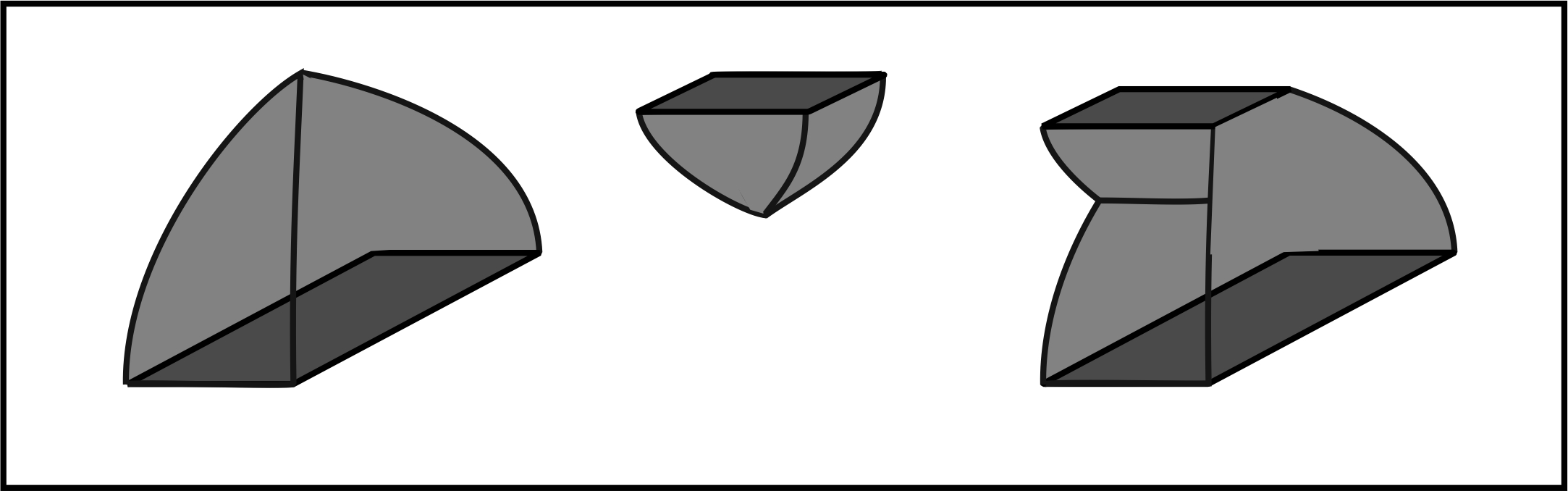
Figure 5. First we see a pair of flat tori, $M_{i}=(M,g_{i})$, isometrically embedded in their own hemispherical suspensions. Then they both isometrically embed into a common $M^{\prime}$.

Example 4.3.

Let $M=S^{1}\times[0,1]$ and let $g_{i}=a_{i}^{2}d\theta^{2}+b_{i}^{2}dl^{2}$, where $a_{1}>a_{2}>0$ and $b_{2}>b_{1}>0$. Take

(4.5) $$D_{i}=\operatorname{diam}_{g_{i}}(M_{i})=\sqrt{(\pi a_{i})^{2}+b_{i}^{2}}.$$

By Proposition 4.2, we know that if we can find $t_{i}\in\mathbb{R}$ and functions $a,b:[t_{1},t_{2}]\to\mathbb{R}$ such that

(4.6) $$a(t) \geq \max_{i=1,2}a_{i}h_{i}(t)$$

(4.7) $$b(t) \geq \max_{i=1,2}b_{i}h_{i}(t)$$

where $h_{i}(t)=\max\{\cos((t-t_{i})\pi/D_{i}),0\}$ and

(4.8) $$a(t_{1})=a_{1},\,\,a(t_{2})=a_{2},\,\,b(t_{1})=b_{1}\,\,\textrm{ and }b(t_{2})=b_{2},$$

then we have isometric embeddings $\varphi_{i}:(M,g_{i})\to(M^{\prime},g^{\prime})$ where

(4.9) $$g^{\prime}=dt^{2}+a^{2}(t)d\theta^{2}+b^{2}(t)dl^{2}.$$

To obtain (4.8), we must choose $t_{2}-t_{1}$ sufficiently large that

(4.10) $$a_{1}h_{1}(t_{2}-t_{1})\leq a_{2}\textrm{ and }b_{2}h_{2}(t_{2}-t_{1})\leq b_{1}.$$

Since $a_{2}/a_{1},b_{2}/b_{1}<1$ this is achieved by taking

(4.11) $$|t_{2}-t_{1}|\geq\max\left\{\frac{D_{1}}{\pi}\arccos\left(\frac{a_{2}}{a_{1}}\right),\frac{D_{2}}{\pi}\arccos\left(\frac{b_{1}}{b_{2}}\right)\right\}.$$

See Figure 5.

Before we prove the proposition we prove the following lemma. Recall that equators in spheres isometrically embed into the hemispheres. Here we create standard isometric embeddings of Riemannian manifolds into hemispherically warped product spaces. The idea comes from Gromov’s notions in filling Riemannian manifolds [Gro83].

Lemma 4.4.

Given a compact Riemannian manifold $(M,g)$ and $D>0$. Let $M^{\prime}=M\times[0,D/2]$ and let $\varphi:M\to M^{\prime}$ be defined by $\varphi(p)=(p,0)$. If a metric $g^{\prime}$ on $M^{\prime}$ satisfies

(4.12) $$g^{\prime}\geq dt^{2}+\cos^{2}(t\pi/D)g\textrm{ on }M^{\prime}$$

and

(4.13) $$g^{\prime}=dt^{2}+g\textrm{ on }M\times\left\{0\right\}\subset M^{\prime}$$

then any geodesic, $\gamma:[0,1]\to M$, of length $\leq D$ satisfies (4.1). If $\operatorname{diam}(M)\leq D$ then $\varphi$ is an isometric embedding.

Here the hemispherical suspension, $M^{\prime}$, is a well defined metric space but not necessarily a smooth manifold as can be seen, for example, on the left side of Figure 6. The inspiration for using a hemispherical suspension comes from Gromov’s work on filling Riemannian manifolds [Gro83].

Proof.

Assume not. There exists a geodesic $\gamma:[0,1]\to M$ of length $\leq D$, and a curve $\sigma:[0,1]\to M^{\prime}$ running from $\gamma(0)$ to $\gamma(1)$ of length $L_{g^{\prime}}(\sigma)<L_{g}(\gamma)$. If we replace the metric $g^{\prime}$ by $g^{\prime\prime}=dt^{2}+\cos^{2}(t\pi/D)g$, then $L_{g^{\prime\prime}}(\sigma)<L_{g}(\gamma)$.

So there exists a curve $C(s)=(x(s),t(s))\in M\times[0,D/2]$ which is minimizing with respect to $g^{\prime\prime}$ between its endpoints $C(0)=(x(0),0)=\gamma(0)$ and $C(1)=(x(1),0)=\gamma(1)$ such that

(4.14) $$L_{g^{\prime\prime}}(C)\leq L_{g^{\prime\prime}}(\sigma)\leq L_{g^{\prime}}(\sigma)<L_{g}(\gamma)=d_{M}(x(0),x(1))\leq D.$$

Since $C:[0,1]\to M^{\prime}$ is a minimizing geodesic in the warped product, $x:[0,1]\to M$, is a minimizing geodesic in $M$. We choose the parameter $s$ so that $x$ is parametrized proportional to arclength and let $h$ be the length of the geodesic $x$, so we have $h=d_{M}(x(0),x(1))\leq D$. See Figure 6.

Figure 6. On the left we have a smooth torus, $M^{m}$, which is warped with a cosine function to create the curved manifold, $M^{m}\times[0,D/2]$, in which $C$ lies. On the right we see the the set $U$ viewed as a subset of a hemisphere created using the same warping function.

Observe that $F:[0,h]\times[0,D/2]\to M^{\prime}$ defined by $F(s,t)=(x(s/h),t)$ is an isometric embedding of a region, $U$, in the standard round sphere, $S^{2}$, of diameter $D$ into $M^{\prime}$. That is the metric on $U$ is

(4.15) $$dt^{2}+\cos^{2}(t\pi/D)ds^{2}$$

and for any curve $\gamma:[a,b]\to U$ where $\gamma(u)=(\gamma_{s}(u),\gamma_{t}(u))$ we have, by (4.12),

$$g^{\prime\prime}((F\circ\gamma)^{\prime}(u),(F\circ\gamma)^{\prime}(u)) = (dt^{2}+\cos^{2}(t\pi/D)g)((F\circ\gamma)^{\prime}(u),F\circ\gamma)^{\prime}(u))$$

$$= \gamma_{t}^{\prime}(u)^{2}+\cos^{2}(t\pi/D)g((x\circ\gamma_{s})^{\prime}(u/h),(x\circ\gamma_{s})^{\prime}(u/h))/h^{2}$$

$$= \gamma_{t}^{\prime}(u)^{2}+\cos^{2}(t\pi/D)|\gamma_{s}^{\prime}(u)|^{2}g(x^{\prime}(u/h),x^{\prime}(u/h))/h^{2}$$

$$= \gamma_{t}^{\prime}(u)^{2}+\cos^{2}(t\pi/D)|\gamma_{s}^{\prime}(u)|^{2}\textrm{ because }g(x^{\prime},x^{\prime})=h^{2}$$

$$= (dt^{2}+\cos^{2}(t\pi/D)ds^{2})(\gamma^{\prime}(u),\gamma^{\prime}(u)).$$

In particular, $L(F\circ x)=L(x)$ by (4.13).

Furthermore $C(s)\subset F(U)$. So $F^{-1}\circ C$ is a curve in $S^{2}$ running between $F^{-1}(C(0))$ and $F^{-1}(C(1))$. Thus

(4.16) $$L_{g^{\prime\prime}}(C)\geq d_{S^{2}}(F^{-1}(C(0)),F^{-1}(C(1)))=L(F^{-1}\circ x)=d_{M}(x(0),x(1))$$

because $F^{-1}\circ x$ runs along a great circle in $S^{2}$ and has length $<D$. This contradicts (4.14). ∎

We may now apply Lemma 4.4 to prove Proposition 4.2:

Proof.

By Lemma 4.4, (4.2) and (4.3), we see that any geodesic, $\gamma:[0,1]\to M_{i}$, of length $\leq D_{i}$ satisfies (4.1).

Given $q_{1},q_{2}\in M$, let $\gamma:[0,1]\to M^{\prime}$ be a length minimizing geodesic from $\varphi_{1}(q_{1})$ to $\varphi_{2}(q_{2})$. So

(4.17) $$\gamma(s)=(c(s),t(s))\in M\times[t_{1},t_{2}].$$

For $f_{i}(t)=\cos((t-t_{i})\pi/D_{i})$

$$L_{g^{\prime}}(\gamma) = \int_{0}^{1}g^{\prime}(\gamma^{\prime}(s),\gamma^{\prime}(s))\,ds$$

$$\geq \int_{0}^{1}\sqrt{t^{\prime}(s)^{2}+\max_{i=1,2}f_{i}^{2}(t(s))g_{i}(c^{\prime}(s),c^{\prime}(s))}\,ds$$

$$\geq \int_{0}^{1}\sqrt{t^{\prime}(s)^{2}+f_{1}^{2}(t(s))g_{1}(c^{\prime}(s),c^{\prime}(s))}\,ds$$

$$\geq \int_{0}^{1}\sqrt{t^{\prime}(s)^{2}+f_{1}^{2}(t(s))g_{1}(\bar{c}^{\prime}(s),\bar{c}^{\prime}(s))}\,ds$$

where $\bar{c}$ is a length minimizing geodesic in $(M,g_{1})$ from $c(0)$ to $c(1)$ parametrized proportional to arclength of length $h=d_{g_{1}}(c(0),c(1))$. Thus

(4.18) $$L_{g^{\prime}}(\gamma)\geq\int_{0}^{1}\sqrt{t^{\prime}(s)^{2}+f_{1}^{2}(t(s))h^{2}}\,ds.$$

This integral is the length of a curve in a hemisphere of diameter $D_{1}$ running from a point $(0,h)$ on the equator to a point $(|t_{1}-t_{2}|,0)$. So it is greater than or equal to the length of the third side of a triangle opposite a right angle with legs of length $d_{M_{1}}(q_{1},q_{2})$ and $|t_{1}-t_{2}|$. Applying the Spherical Law of Cosines rescaled we obtain

(4.19) $$d_{M^{\prime}}(\varphi_{1}(q_{1}),\varphi_{2}(q_{2})) \geq \frac{D_{1}}{\pi}\arccos\left(\cos\left(\frac{\pi d_{M_{1}}(q_{1},q_{2})}{D_{1}}\right)\cos\left(\frac{\pi|t_{1}-t_{2}|}{D_{1}}\right)\right)$$

(4.20) $$\geq d_{M_{1}}(q_{1},q_{2}).$$

∎

4.2. Estimating Distances between Manifolds

The Gromov-Hausdorff distance between a pair of metric spaces was estimated in terms of the Lipschitz distance between them in [Gro99]. In [SW11], the intrinsic flat distance between a pair of integral current spaces was estimated in terms of the Lipschitz distance between them. Here we give a simple proof estimating these distances between Riemannian manifolds using explicit isometric embeddings into a common Riemannian manifold. Recall Definitions 2.7 and 2.9.

Lemma 4.5.

Suppose $M_{1}=(M,g_{1})$ and $M_{2}=(M,g_{2})$ are diffeomorphic oriented precompact Riemannian manifolds and suppose there exists $\epsilon>0$ such that

(4.21) $$g_{1}(V,V)<(1+\epsilon)^{2}g_{2}(V,V)\textrm{ and }g_{2}(V,V)<(1+\epsilon)^{2}g_{1}(V,V)\qquad\forall\,V\in TM.$$

Then for any

(4.22) $$a_{1}>\frac{\arccos(1+\epsilon)^{-1}}{\pi}\operatorname{diam}(M_{2})$$

and

(4.23) $$a_{2}>\frac{\arccos(1+\epsilon)^{-1}}{\pi}\operatorname{diam}(M_{1}),$$

there is a pair of isometric embeddings $\varphi_{i}:M_{i}\to M^{\prime}=\bar{M}\times[t_{1},t_{2}]$ with a metric as in Proposition 4.2 where $t_{2}-t_{1}\geq\max\left\{a_{1},a_{2}\right\}$.

Thus the Gromov-Hausdorff distance between the metric completions is bounded,

(4.24) $$d_{GH}(\bar{M}_{1},\bar{M}_{2})\leq a:=\max\left\{a_{1},a_{2}\right\},$$

and the intrinsic flat and scalable intrinsic flat distances between the settled completions are bounded,

(4.25) $$d_{\mathcal{F}}(M^{\prime}_{1},M^{\prime}_{2})\leq a\left(V_{1}+V_{2}+A_{1}+A_{2}\right),$$

(4.26) $$d_{s\mathcal{F}}(M^{\prime}_{1},M^{\prime}_{2})\leq\left(a(V_{1}+V_{2})\right)^{1/(m+1)}+\left(a(A_{1}+A_{2})\right)^{1/(m)}$$

where $V_{i}=\operatorname{Vol}_{m}(M_{i})$ and $A_{i}=\operatorname{Vol}_{m-1}(\partial M_{i})$.

Proof.

By our choice of $a_{i}$ we have

(4.27) $$g_{1}(V,V)>\cos^{2}(a_{1}\pi/diam(M_{2}))g_{2}(V,V)\qquad\forall V\in TM$$

and

(4.28) $$g_{2}(V,V)>\cos^{2}(a_{2}\pi/\operatorname{diam}(M_{1}))g_{1}(V,V)\qquad\forall V\in TM.$$

Applying Proposition 4.2 and setting $t_{1}=0$ and $t_{2}=a$, we have isometric embeddings $\varphi_{i}:(M,g_{i})\to(M^{\prime},g^{\prime})$ for any $g^{\prime}$ satisfying (4.2) and (4.3). In fact, the metric $g^{\prime}$ on $M^{\prime}$ can be chosen so that

(4.29) $$g^{\prime}(V,V)\leq dt^{2}(V,V)+g_{1}(V,V)+g_{2}(V,V)\qquad\forall\,V\in TM^{\prime}.$$

By Definition 2.5 we have,

(4.30) $$d_{GH}(\bar{M}_{1},\bar{M}_{2})\leq d^{M^{\prime}}_{H}(\varphi_{1}(M_{1}),\varphi_{2}(M_{2})).$$

For all $r>a$, $\varphi_{1}(M_{1})\subset T_{r}(\varphi_{2}(M_{2}))$ and $\varphi_{2}(M_{2})\subset T_{r}(\varphi_{1}(M_{1}))$, because for all $p\in M$ we have

(4.31) $$d_{M^{\prime}}(\varphi_{1}(p),\varphi_{2}(p))=|t_{2}-t_{1}|=a.$$

By Definition 2.4 we have (4.24).

Recall that to estimate the Intrinsic flat Distance and scalable intrinsic flat distance we must estimate volumes of a filling manifold and an excess boundary as in (2.12) and (2.21). Taking $\nu$ to be the unit inward normal to $\partial M^{\prime}\setminus(M_{1}\cup M_{2})$ and applying the estimate on $g^{\prime}$ given in (4.29) we have

$$d_{\mathcal{F}}(M^{\prime}_{1},M^{\prime}_{2}) \leq \operatorname{Vol}(M^{\prime})+\operatorname{Vol}(\partial M^{\prime}\setminus(M_{1}\cup M_{2}))$$

$$= \int_{t_{1}}^{t_{2}}\int_{M}\mu_{g^{\prime}}\,dt+\int_{t_{1}}^{t_{2}}\int_{\partial M}\nu\lrcorner\mu_{g^{\prime}}\,dt$$

$$\leq |t_{2}-t_{1}|(\operatorname{Vol}(M_{1})+\operatorname{Vol}(M_{2}))+|t_{2}-t_{1}|(\operatorname{Vol}(\partial M_{1})+\operatorname{Vol}(\partial M_{2})).$$

and

$$d_{s\mathcal{F}}(M^{\prime}_{1},M^{\prime}_{2}) \leq \left(\operatorname{Vol}(M^{\prime})\right)^{1/(m+1)}+\left(\operatorname{Vol}(\partial M^{\prime}\setminus(M_{1}\cup M_{2}))\right)^{1/m}$$

$$= \left(\int_{t_{1}}^{t_{2}}\int_{M}\mu_{g^{\prime}}\,dt\right)^{1/(m+1)}+\left(\int_{t_{1}}^{t_{2}}\int_{\partial M}\nu\lrcorner\mu_{g^{\prime}}\,dt\right)^{1/m}$$

$$\leq \left(|t_{2}-t_{1}|(\operatorname{Vol}(M_{1})+\operatorname{Vol}(M_{2}))\right)^{1/(m+1)}$$

$$\qquad+\left(|t_{2}-t_{1}|(\operatorname{Vol}(\partial M_{1})+\operatorname{Vol}(\partial M_{2}))\right)^{1/m}.$$

∎

4.3. Appending Regions without Smooth Approximations

Now we examine pairs of precompact oriented manifolds $(M_{1},g_{1})$ and $(M_{2},g_{2})$ which are not diffeomorphic but have diffeomorphic regions $U_{i}\subset M_{i}$. That is, there is a common smooth manifold with boundary $U$ and diffeomorphisms $\psi_{i}:U\to U_{i}\subset M_{i}$. Then we may apply Proposition 4.2 and Lemma 4.5 to the regions $U_{i}$ to estimate the distances between the metric and settled completions of the $M_{i}$. Recall also Definitions 2.7 and 2.9. Recall also the distinction between the intrinsic length metric, $d_{U}$, and the restricted metric $d_{M}$, on a region $U\subset M$ and the corresponding diameters, $\operatorname{diam}_{M}(U)\leq\operatorname{diam}_{U}(U)$, in Definition 2.1.

Theorem 4.6.

Suppose $M_{1}=(M,g_{1})$ and $M_{2}=(M,g_{2})$ are oriented precompact Riemannian manifolds with diffeomorphic subregions $U_{i}\subset M_{i}$ and diffeomorphisms $\psi_{i}:U\to U_{i}$ such that

(4.32) $$\psi_{1}^{*}g_{1}(V,V)<(1+\epsilon)^{2}\psi_{2}^{*}g_{2}(V,V)\qquad\forall\,V\in TU$$

and

(4.33) $$\psi_{2}^{*}g_{2}(V,V)<(1+\epsilon)^{2}\psi_{1}^{*}g_{1}(V,V)\qquad\forall\,V\in TU.$$

Taking the extrinsic diameters,

(4.34) $$D_{U_{i}}=\sup\{\operatorname{diam}_{M_{i}}(W):\,W\textrm{ is a connected component of }U_{i}\}\leq\operatorname{diam}(M_{i}),$$

we define a hemispherical width,

(4.35) $$a>\frac{\arccos(1+\epsilon)^{-1}}{\pi}\max\{D_{U_{1}},D_{U_{2}}\}.$$

Taking the difference in distances with respect to the outside manifolds,

(4.36) $$\lambda=\sup_{x,y\in U}|d_{M_{1}}(\psi_{1}(x),\psi_{1}(y))-d_{M_{2}}(\psi_{2}(x),\psi_{2}(y))|,$$

we define heights,

(4.37) $$h=\sqrt{\lambda(\max\{D_{U_{1}},D_{U_{2}}\}+\lambda/4)\,}$$

and

(4.38) $$\bar{h}=\max\{h,\sqrt{\epsilon^{2}+2\epsilon}\;D_{U_{1}},\sqrt{\epsilon^{2}+2\epsilon}\;D_{U_{2}}\}.$$

Then the Gromov-Hausdorff distance between the metric completions is bounded,

(4.39) $$d_{GH}(\bar{M}_{1},\bar{M}_{2})\leq a+2\bar{h}+\max\left\{d^{M_{1}}_{H}(U_{1},M_{1}),d^{M_{2}}_{H}(U_{2},M_{2})\right\}$$

and the intrinsic flat distance between the settled completions is bounded,

$$d_{\mathcal{F}}(M^{\prime}_{1},M^{\prime}_{2}) \leq \left(2\bar{h}+a\right)\Big{(}\operatorname{Vol}_{m}(U_{1})+\operatorname{Vol}_{m}(U_{2})+\operatorname{Vol}_{m-1}(\partial U_{1})+\operatorname{Vol}_{m-1}(\partial U_{2})\Big{)}$$

$$+\operatorname{Vol}_{m}(M_{1}\setminus U_{1})+\operatorname{Vol}_{m}(M_{2}\setminus U_{2}).$$

and the scalable intrinsic flat distance is bounded,

$$d_{s\mathcal{F}}(M^{\prime}_{1},M^{\prime}_{2}) \leq \Big{(}(\operatorname{Vol}_{m}(U_{1})+\operatorname{Vol}_{m}(U_{2}))\left(\bar{h}+a\right)\Big{)}^{1/(m+1)}$$

$$+\,\,\Big{(}\,\big{(}2\bar{h}+a\big{)}(\operatorname{Vol}_{m-1}(\partial U_{1})+\operatorname{Vol}_{m-1}(\partial U_{2}))$$

$$\qquad+\operatorname{Vol}_{m}(M_{1}\setminus U_{1})+\operatorname{Vol}_{m}(M_{2}\setminus U_{2})\,\Big{)}^{1/m}.$$

Figure 2 may be viewed as an application of this theorem. It should be noted that this theorem is an improvement on the Bridge Method Lemma A.2 of [SW11] in two respects. First, we allow $U_{1}$ and $U_{2}$ not isometric, and secondly we loosen the diameter bounds of that method asking only for control on the $\lambda$ defined here.

Recall in Definition 2.1, that two different metrics are defined on a connected subdomain, $U\subset M$. When $U$ is also totally convex, these two metrics agree. Theorem 4.6 does not require the subdomains to be connected or convex, and so the proof becomes quite difficult. Before we prove this theorem we state and prove a special case with stronger estimates.

Theorem 4.7.

Suppose $M_{1}=(M,g_{1})$ and $M_{2}=(M,g_{2})$ are oriented Riemannian manifolds with diffeomorphic totally convex subregions $U_{i}\subset M_{i}$ and diffeomorphisms $\psi_{i}:U\to U_{i}$ such that

(4.40) $$\psi_{1}^{*}g_{1}(V,V)<(1+\epsilon)^{2}\psi_{2}^{*}g_{2}(V,V)\qquad\forall\,V\in TU$$

and

(4.41) $$\psi_{2}^{*}g_{2}(V,V)<(1+\epsilon)^{2}\psi_{1}^{*}g_{1}(V,V)\qquad\forall\,V\in TU.$$

Then for any

(4.42) $$a_{1}>\frac{\arccos(1+\epsilon)^{-1}}{\pi}\operatorname{diam}_{U_{2}}(U_{2})$$

and

(4.43) $$a_{2}>\frac{\arccos(1+\epsilon)^{-1}}{\pi}\operatorname{diam}_{U_{1}}(U_{1}),$$

there is a pair of isometric embeddings $\varphi_{i}:U_{i}\to M^{\prime}$ where $M^{\prime}=U\times[t_{1},t_{2}]$ where $t_{2}-t_{1}=\max\left\{a_{1},a_{2}\right\}$ such that $\varphi_{i}(x)=(x,t_{i})$. Furthermore, these isometric embeddings extend to isometric embeddings $\varphi:M_{i}\to Z^{\prime}$, where $Z^{\prime}$ is a length metric space defined by gluing $M_{i}$ to $M^{\prime}$ along $U_{i}$.

In particular the Gromov-Hausdorff distance between the metric completions is bounded,

(4.44) $$d_{GH}(\bar{M}_{1},\bar{M}_{2})\leq\max\left\{a_{1},a_{2}\right\}+\max\left\{d^{M_{1}}_{H}(U_{1},M_{1}),d^{M_{2}}_{H}(U_{2},M_{2})\right\}$$

and the intrinsic flat distance between the settled completions is bounded,

$$d_{\mathcal{F}}(M^{\prime}_{1},M^{\prime}_{2}) \leq \max\left\{a_{1},a_{2}\right\}\Big{(}\operatorname{Vol}(U_{1})+\operatorname{Vol}(U_{2})+\operatorname{Vol}(\partial U_{1})+\operatorname{Vol}(\partial U_{2})\Big{)}$$

$$+\operatorname{Vol}(M_{1}\setminus U_{1})+\operatorname{Vol}(M_{2}\setminus U_{2}),$$

and the scalable intrinsic flat distance is bounded,

$$d_{s\mathcal{F}}(M^{\prime}_{1},M^{\prime}_{2})\,\,\leq\,\,\Big{(}\,\max\left\{a_{1},a_{2}\right\}(\operatorname{Vol}(U_{1})+\operatorname{Vol}(U_{2}))\,\Big{)}^{1/(m+1)}\qquad\qquad\qquad\qquad$$

$$\qquad+\,\,\Big{(}\,\max\left\{a_{1},a_{2}\right\}(\operatorname{Vol}(\partial U_{1})+\operatorname{Vol}(\partial U_{2}))+\operatorname{Vol}(M_{1}\setminus U_{1})+\operatorname{Vol}(M_{2}\setminus U_{2})\,\Big{)}^{1/(m)}.$$

Proof.

The metric $g^{\prime}$ on $M^{\prime}$ is defined by applying Proposition 4.2 and Lemma 4.5 to the diffeomorphic regions, $U_{1}$ and $U_{2}$; taking $D_{i}=\operatorname{diam}_{U_{i}}(U_{i})$ as defined above, $\varphi_{i}:U_{i}\to M^{\prime}$ are isometric embeddings. We can choose $g^{\prime}$ satisfying (4.29).

We must verify that the $M_{i}$ isometrically embed into $Z^{\prime}$ constructed as in the statement of the theorem. To see this we take any $x,y\in M_{1}$ and a shortest curve $C\subset Z^{\prime}$ running between $\varphi_{1}(x)$ and $\varphi_{1}(y)$. If the curve never enters $\varphi_{2}(M_{2}\setminus U_{2})$ then $d_{M_{1}}(x,y)=d_{Z^{\prime}}(\varphi_{1}(x),\varphi_{1}(y))$ by Lemma 4.5 and Lemma A.1 in the Appendix of [SW11] applied to $\varphi_{1}(M_{1})\cup M^{\prime}\subset Z^{\prime}$. If the curve does enter $\varphi_{2}(M_{2}\setminus U_{2})$ then we have a length minimizing curve which leaves $\bar{U}_{2}$ contradicting the fact that it is convex. The same argument may be repeated to prove $\varphi_{2}:M_{2}\to Z^{\prime}$ is an isometric embedding.

So now we may estimate the Gromov-Hausdorff distance as in Remark 2.6. Let $r_{i}=d^{M_{i}}_{H}(M_{i},U_{i})$. We claim

(4.45) $$d_{GH}(M_{1},M_{2})\leq d^{Z^{\prime}}_{H}\big{(}\varphi_{1}(M_{1}),\varphi_{2}(M_{2})\big{)}\leq|t_{1}-t_{2}|+\max\left\{r_{i}\right\}.$$

Fix any $\delta>0$. Then any point $p\in M_{1}$ has a point $q\in U_{1}$ such that $d(p,q)\leq r_{1}+\delta$. Furthermore, $\varphi_{1}(q)=(q,t_{1})\in M^{\prime}\subset Z^{\prime}$ so

(4.46) $$d_{Z^{\prime}}(\varphi_{1}(q),(q,t_{2}))=|t_{2}-t_{1}|$$

and $(q,t_{2})\subset\varphi_{2}(U_{2})\subset\varphi_{2}(M_{2})$. Thus

(4.47) $$\varphi_{1}(M_{1})\subset T_{r_{1}+\delta+|t_{2}-t_{1}|}(\varphi(M_{2}))$$

and similarly

(4.48) $$\varphi_{2}(M_{2})\subset T_{r_{2}+\delta+|t_{2}-t_{1}|}(\varphi(M_{1})).$$

The claim follows by taking $\delta\to 0$.

We bound the intrinsic flat distance as in Remark 2.8 taking $M^{\prime}$ to be the filling manifold with the metric $g^{\prime}$ defined in Lemma 4.5 satisfying (4.29). We apply the same estimates as in Lemma 4.5 to bound the volumes of these regions, only now we add in the additional volume terms coming from the additional components of the excess boundary $M_{i}\setminus U_{i}$.

We bound the scalable intrinsic flat distance as in Remark 2.11. Again we include the additional components of the excess boundary but insert them into the summand with an exponent of $1/m$ since these are $m$ dimensional boundary regions and the scalable flat distance is 1 dimensional. ∎

We now prove Theorem 4.6. To prove this theorem we adapt the proof of the convex case and the proof of Lemma A.2 in [SW11]. It is essential to possibly push the two manifolds further apart than required simply to isometrically embed the $U_{i}$ into $M^{\prime}$ as a short cut for a path between points in $\varphi_{1}(M_{1})$ might be found within $\varphi_{2}(M_{2}\setminus U_{2})$.

Proof.

For each corresponding pair of connected components $U_{\alpha,i}$ of $U_{i}$, we create a hemispherically defined filling bridge $M^{\prime}_{\alpha}$ diffeomorphic to $U_{\alpha_{i},i}\times[0,a]$ with metric $g^{\prime}_{\alpha}$ satisfying (4.1) by applying Proposition 4.2 and Lemma 4.5 using the $a_{i}=a_{i}(\alpha)$ defined there for that particular connected component, $U_{\alpha}$ and $D_{i}=D_{U_{i}}$. Observe that all $a_{i}\leq a$, so we may take $|t_{1}-t_{2}|=a$ for all the connected components. Any minimal geodesic $\gamma:[0,1]\to U_{\alpha,i}$ of length $\leq D_{U_{i}}\leq\operatorname{diam}_{M_{i}}(U_{i})$ satisfies (4.1).

We take the disjoint unions of these bridges to be $M^{\prime}$. So it has a metric $g^{\prime}$ satisfying (4.29). Observe that the boundary of $M^{\prime}$ is $(U,g_{1})\cup(U,g_{2})\cup(\partial U\times[0,a],g^{\prime})$. So that

(4.49) $$\operatorname{Vol}_{m}(M^{\prime}) = \sum_{\alpha}\operatorname{Vol}_{m}(M_{\alpha}^{\prime})$$

(4.50) $$\leq \sum_{\alpha}a(\operatorname{Vol}_{m}(U_{\alpha,1})+\operatorname{Vol}_{m}(U_{\alpha,2}))$$

(4.51) $$\leq a(\operatorname{Vol}_{m}(U_{1})+\operatorname{Vol}_{m}(U_{2}))$$

and

(4.52) $$\operatorname{Vol}_{m}\left(\partial M^{\prime}\setminus(\varphi_{1}(U_{1})\cup\varphi_{2}(U_{2})\right)\leq a\;(\operatorname{Vol}_{m-1}(\partial U_{1})+\operatorname{Vol}_{m-1}(\partial U_{2}))$$

as in Lemma 4.5.

We cannot directly glue $M_{i}$ to $M^{\prime}$ and obtain an isometric embedding because our regions are not convex. On either end of the filling bridges, we glue isometric products $U_{\alpha}\times[0,\bar{h}]$ with metric $dt^{2}+g_{i}$, so that all the bridges are extended by an equal length on either side. This creates a Lipschitz manifold,

(4.53) $$M^{\prime\prime}=(U_{1}\times[0,\bar{h}])\sqcup_{U_{1}}M^{\prime}\sqcup_{U_{2}}(U_{2}\times[0,\bar{h}]).$$

We then define $\varphi_{i}:U_{i}\to M^{\prime\prime}$ such that

(4.54) $$\varphi_{1}(x) = (x,0)\in U_{1}\times[0,\bar{h}]$$

(4.55) $$\varphi_{2}(x) = (x,\bar{h})\in U_{2}\times[0,\bar{h}]$$

as in Figure 7. Then by (4.49) and (4.52), we have

(4.56) $$\operatorname{Vol}_{m+1}(M^{\prime\prime}) = \operatorname{Vol}_{m+1}(M^{\prime})+\bar{h}(\operatorname{Vol}_{m}(U_{1})+\operatorname{Vol}_{m}(U_{2}))$$

(4.57) $$\leq (a+\bar{h})(\operatorname{Vol}_{m}(U_{1})+\operatorname{Vol}_{m}(U_{2}))$$

and $\operatorname{Vol}_{m}\left(\partial M^{\prime\prime}\setminus(\varphi_{1}(U_{1})\cup\varphi_{2}(U_{2})\right)=$

(4.58) $$= \operatorname{Vol}_{m}\left(\partial M^{\prime}\setminus(\varphi_{1}(U_{1})\cup\varphi_{2}(U_{2})\right)+\bar{h}(\operatorname{Vol}_{m-1}(\partial U_{1})+\operatorname{Vol}_{m-1}(\partial U_{2}))$$

(4.59) $$\leq (a+\bar{h})(\operatorname{Vol}_{m-1}(\partial U_{1})+\operatorname{Vol}_{m-1}(\partial U_{2})).$$

Finally we glue $M_{1}$ and $M_{2}$ to the far ends of $M^{\prime\prime}$ along $\varphi_{i}(U_{i})$ to create a connected length space

(4.60) $$Z=\bar{M}_{1}\sqcup_{U_{1}}M^{\prime\prime}\sqcup_{U_{2}}\bar{M}_{2}$$

where distances in $Z$ are defined by taking the infimum of lengths of curves as usual. See Figure 7. We will refer to each connected component, $M^{\prime\prime}_{\alpha}$ of $M^{\prime\prime}$ as the filling bridge corresponding to $U_{\alpha}$.

Figure 7. Creating $Z$ for Theorem 4.6.

We must prove that $\varphi_{1}:M_{1}\to Z$ mapping $M_{1}$ into its copy in $Z$ is an isometric embedding. To see this we take any $x,y\in M_{1}$ and a shortest curve $C\subset Z$ running between $\varphi_{1}(x)$ and $\varphi_{1}(y)$. As in the convex proof, our only concern is the possibility that $C$ passes into $\varphi_{2}(M_{2}\setminus U_{2})$.

If the minimizing curve never crosses a filling bridge, then we claim it has the same length as a curve in $\varphi_{1}(M_{1})$. To see this, we take any $s_{2}>s_{1}\in[0,1]$ such that $C(s_{1}),C(s_{2})\in\varphi_{1}(M_{1})$ and $C((s_{1},s_{2}))\subset Z\setminus\varphi_{1}(M_{1})$. Since $C$ is assumed not to cross a bridge (not to enter $\varphi_{2}(M_{2})$, then $C(s_{1})=\varphi(x_{1})$ and $C(s_{2})=\varphi(x_{2})$ where $x_{1},x_{2}$ lie in the same connected component, $U_{\alpha,1}$, of $U_{1}$. Since $C([s_{1},s_{2}])$ is a minimizing curve it has length

(4.61) $$\leq d_{M^{\prime\prime}}(C(s_{1}),C(s_{2}))\leq d_{M_{1}}(x_{1},x_{2})\leq\operatorname{diam}_{M_{1}}(U_{\alpha,1})\leq D_{U_{1}}.$$

By (4.1), a minimal geodesic from $x_{1}$ to $x_{2}$ lying in $U_{\alpha,1}$ has the same length as $C([s_{1},s_{2}])$. So we may replace this segment of $C$ with the image of this minimal geodesic.

On the other hand, if the minimizing curve crosses a filling bridge all the way to $\varphi_{2}(M_{2})$, then we may carefully apply the choice of $\bar{h}$ to reach a contradiction as in the left hand side of Figure 8. We define the following points $0\leq t_{1}<t_{2}\leq t_{3}<t_{4}\leq 1$ such that

(4.62) $$t_{1} = \inf\{t:\,\,C(t)\in Cl(Z\setminus\varphi_{1}(M_{1}))\},$$

(4.63) $$t_{2} = \min\{t:\,\,C(t)\in\varphi_{2}(M_{2})\},$$

(4.64) $$t_{4} = \min\{t>t_{2}:\,\,C(t)\in\varphi_{1}(M_{1})\},$$

(4.65) $$t_{3} = \max\{t\in[t_{2},t_{4}):\,\,C(t)\in\varphi_{2}(M_{2})\}$$

so that $C([t_{1},t_{2}])$ and $C([t_{3},t_{4}])$ are geodesic segments lying within filling bridges:

(4.66) $$C([t_{1},t_{2}])\subset M^{\prime\prime}_{\alpha_{1,2}}\qquad C([t_{3},t_{4}])\subset M^{\prime\prime}_{\alpha_{3,4}}.$$

Figure 8. Why length minimizing curves cannot cross bridges in the proof of Theorem 4.6.

Observe that there are points $p_{1},p_{4}\in U$ and $p_{2},p_{3}\in\partial(U)$ such that

(4.67) $$\varphi_{1}(\psi_{1}(p_{1}))=C(t_{1}) \varphi_{1}(\psi_{1}(p_{4}))=C(t_{4})$$

(4.68) $$\varphi_{2}(\psi_{2}(p_{2}))=C(t_{2}) \varphi_{2}(\psi_{2}(p_{3}))=C(t_{3}).$$

Observe that since $C([t_{2},t_{3}])\subset\varphi_{2}(M_{2})$ we know the length of this segment is

(4.69) $$d_{Z}(C(t_{2}),C(t_{3}))=d_{M_{2}}(\psi_{2}(p_{2}),\psi_{2}(p_{3}))\geq d_{M_{1}}(\psi_{1}(p_{2}),\psi_{1}(p_{3}))-\lambda$$

by the definition of $\lambda$ in (4.36).

We claim that the lengths of the other segments are

(4.70) $$d_{M^{\prime\prime}}(C(t_{1}),C(t_{2}))>\sqrt{d_{M_{1}}(p_{1},p_{2})^{2}+h^{2}\,}$$

and

(4.71) $$d_{M^{\prime\prime}}(C(t_{3}),C(t_{4}))>\sqrt{d_{M_{1}}(p_{3},p_{4})^{2}+h^{2}\,}.$$

Once we prove this claim, we see that by the definition of $h$ we have

(4.72) $$d_{M^{\prime\prime}}(C(t_{1}),C(t_{2})) > d_{M_{1}}(p_{1},p_{2})+\lambda/2,$$

(4.73) $$d_{M^{\prime\prime}}(C(t_{3}),C(t_{4})) > d_{M_{1}}(p_{3},p_{4})+\lambda/2.$$

This combined with (4.69) implies that

$$L(C([t_{1},t_{4}]) = d_{M^{\prime\prime}}(C(t_{1}),C(t_{2}))+d_{Z}(C(t_{2}),C(t_{3}))+d_{M^{\prime\prime}}(C(t_{3}),C(t_{4}))$$

$$> d_{M_{1}}(p_{1},p_{2})+\lambda/2+d_{M_{1}}(p_{2},p_{3})-\lambda+d_{M_{1}}(p_{3},p_{4})+\lambda/2$$

$$\geq d_{M_{1}}(p_{1},p_{2})+d_{M_{1}}(p_{2},p_{3})+d_{M_{1}}(p_{3},p_{4})$$

$$\geq d_{M_{1}}(p_{1},p_{4})=d_{\varphi_{1}(M_{1})}(C(t_{1}),C(t_{4}))$$

$$\geq d_{Z}(C(t_{1}),C(t_{4})),$$

which is a contradicts the fact that $C$ was minimizing.

So we need only prove our claim in (4.70) and (4.71) to see that $\varphi_{1}:M_{1}\to Z$ is an isometric embedding. This claim concerns a minimizing geodesic lying in a single connected component of the filling bridges,

(4.74) $$\gamma:[0,1]\to(U_{\alpha,1}\times[0,\bar{h}])\sqcup_{U_{\alpha,1}}M_{\alpha}^{\prime}\sqcup_{U_{\alpha,2}}(U_{\alpha,2}\times[0,\bar{h}])$$

such that

(4.75) $$\gamma(0)=(q_{0},0)\in U_{\alpha,1}\times\{0\}\subset\varphi_{1}(M_{1})$$

and

(4.76) $$\gamma(1)=(q_{3},\bar{h})\in U_{\alpha,2}\times\{\bar{h}\}\subset\varphi_{2}(M_{2}).$$

Consult the right hand side of Figure 8. Let $0<s_{1}<s_{2}<1$ be chosen so that

(4.77) $$\gamma(s_{1})=(q_{1},\bar{h})\in U_{\alpha,1}\times\{\bar{h}\}\subset\partial M_{\alpha}^{\prime}$$

and

(4.78) $$\gamma(s_{2})=(q_{2},0)\in U_{\alpha,2}\times\{0\}\subset\partial M_{\alpha}^{\prime}.$$

Then by (4.4), we have

(4.79) $$L_{g^{\prime}}(\gamma([s_{1},s_{2}])=d_{g^{\prime}}(\gamma(s_{1}),\gamma(s_{2}))\geq d_{g_{1}}(q_{1},q_{2}),$$

so that

$$L(\gamma) = d_{Z}(\gamma(0),\gamma(s_{1}))+d_{Z}(\gamma(s_{1}),\gamma(s_{2}))+d_{Z}(\gamma(s_{2}),\gamma(1))$$

$$= \sqrt{d_{U_{1}}(q_{0},q_{1})^{2}+\bar{h}^{2}}+d_{U_{1}}(q_{1},q_{2})+\sqrt{d_{U_{2}}(q_{2},q_{3})^{2}+\bar{h}^{2}}$$

$$\geq \sqrt{d_{U_{1}}(q_{0},q_{1})^{2}+h^{2}}+d_{U_{1}}(q_{1},q_{2})$$

$$+\qquad\sqrt{d_{U_{1}}(q_{2},q_{3})^{2}/(1+\epsilon)^{2}+(\epsilon^{2}+2\epsilon)D_{U_{1}}^{2}}$$

$$\geq \sqrt{d_{M_{1}}(q_{0},q_{1})^{2}+h^{2}}+d_{M_{1}}(q_{1},q_{2})$$

$$+\qquad\sqrt{d_{M_{1}}(q_{2},q_{3})^{2}/(1+\epsilon)^{2}+(\epsilon^{2}+2\epsilon)d_{M_{1}}(q_{3},q_{4})^{2}}$$

$$\geq \sqrt{d_{M_{1}}(q_{0},q_{1})^{2}+h^{2}}+d_{M_{1}}(q_{1},q_{2})+\sqrt{d_{M_{1}}(q_{2},q_{3})^{2}}$$

$$> \sqrt{(d_{M_{1}}(q_{0},q_{1})+d_{M_{1}}(q_{1},q_{2})+d_{M_{1}}(q_{2},q_{3}))^{2}+h^{2}}$$

$$\geq \sqrt{d_{M_{1}}(q_{0},q_{3})^{2}+h^{2}}.$$

This gives us (4.70) and (4.71). Thus we have proven $\varphi_{1}:M_{1}\to Z$ is an isometric embedding and the same follows for $\varphi_{2}:M_{2}\to Z$.

So now we may estimate the Gromov-Hausdorff distance: Let $r_{i}=d^{M_{i}}_{H}(M_{i},U_{i})$. We claim

(4.80) $$d_{GH}(M_{1},M_{2})\leq d^{Z}_{H}(\varphi_{1}(M_{1}),\varphi_{2}(M_{2})\leq\bar{h}+\bar{h}+a+\max\left\{r_{i}\right\}.$$

Fix any $\delta>0$. Then any point $p\in M_{1}$ has a point $q\in U_{1}$ such that $d(p,q)\leq r_{1}+\delta$. Furthermore,

(4.81) $$d_{Z}(\varphi_{1}(q),\varphi_{2}(q))\leq a+\bar{h}+\bar{h}$$

and $\varphi_{2}(q)\subset\varphi_{2}(U_{2})\subset\varphi_{2}(M_{2})$. Thus

(4.82) $$\varphi_{1}(M_{1})\subset T_{r_{1}+\delta+a+\bar{h}+\bar{h}}(\varphi(M_{2})).$$

and similarly

(4.83) $$\varphi_{2}(M_{2})\subset T_{r_{2}+\delta+a+\bar{h}+\bar{h}}(\varphi(M_{1})).$$

The claim follows by taking $\delta\to 0$.

To bound the intrinsic flat distance and scalable intrinsic flat distance, we take $B^{m+1}=M^{\prime\prime}$ to be the filling manifold and then the excess boundary is

(4.84) $$A^{m}=\varphi_{1}(M_{1}\setminus U_{1})\cup\varphi_{2}(M_{2}\setminus U_{2})\cup\partial M^{\prime\prime}\setminus(\varphi_{1}(U_{1})\cup\varphi_{2}(U_{2}))$$

so that with appropriate orientations we have

(4.85) $$\int_{\varphi_{1}(M_{1})}\omega-\int_{\varphi_{2}(M_{2})}\omega=\int_{B^{m+1}}d\omega+\int_{A^{m}}\omega.$$

The volumes of these manifolds have been computed in (4.58) and (4.56). So as in Remark 2.8 we have

$$d_{\mathcal{F}}(M_{1},M_{2}) \leq \operatorname{Vol}_{m}(U_{1})\left(\bar{h}+a\right)+\operatorname{Vol}_{m}(U_{2})\left(\bar{h}+a\right)$$

$$+\left(\bar{h}+a\right)\operatorname{Vol}_{m-1}(\partial U_{1})+\left(\bar{h}+a\right)\operatorname{Vol}_{m-1}(\partial U_{2})$$

$$+\operatorname{Vol}_{m}(M_{1}\setminus U_{1})+\operatorname{Vol}_{m}(M_{2}\setminus U_{2}).$$

The scalable intrinsic flat distance is bounded as in Remark 2.11 so that we have

$$d_{s\mathcal{F}}(M_{1},M_{2}) \leq \Big{(}\operatorname{Vol}_{m}(U_{1})\left(\bar{h}+a\right)+\operatorname{Vol}_{m}(U_{2})\left(\bar{h}+a\right)\Big{)}^{1/(m+1)}$$

$$+\Big{(}\left(\bar{h}+a\right)\operatorname{Vol}_{m-1}(\partial U_{1})+\left(\bar{h}+a\right)\operatorname{Vol}_{m-1}(\partial U_{2})$$

$$+\operatorname{Vol}_{m}(M_{1}\setminus U_{1})+\operatorname{Vol}_{m}(M_{2}\setminus U_{2})\Big{)}^{1/m}.$$

∎

5. Intrinsic Flat Limits

In this section we examine sequences of Riemannian manifolds which converge smoothly away from singular sets and their intrinsic flat limits proving Theorem 1.3. This theorem will be shown to be consequences of the following more powerful theorem which requires a condition on the embeddings of the exhaustion in the manifold:

Definition 5.1.

Given a sequence of Riemannian manifolds $M_{i}=(M,g_{i})$ and an open subset, $U\subset M$, a connected precompact exhaustion, $W_{j}$, of $U$ satisfying (1.2) is uniformly well embedded if

(5.1) $$\lambda_{i,j,k}=\sup_{x,y\in W_{j}}|d_{(W_{k},g_{i})}(x,y)-d_{(M,g_{i})}(x,y)|$$

has

(5.2) $$\limsup_{j\to\infty}\limsup_{k\to\infty}\limsup_{i\to\infty}\lambda_{i,j,k}=0.$$

and thus a uniform upper bound

(5.3) $$\lambda_{i,j,k}\leq\lambda_{0}<\infty$$

Theorem 5.2.

Let $M_{i}=(M,g_{i})$ be a sequence of compact oriented Riemannian manifolds such that there is a closed subset, $S$, and a uniformly well embedded connected precompact exhaustion, $W_{j}$, of $M\setminus S$ satisfying (1.2) such that $g_{i}$ converge smoothly to $g_{\infty}$ on each $W_{j}$ with

(5.4) $$\operatorname{diam}_{M_{i}}(W_{j})\leq D_{0}\qquad\forall i\geq j,$$

(5.5) $$\operatorname{Vol}_{g_{i}}(\partial W_{j})\leq A_{0}$$

and

(5.6) $$\operatorname{Vol}_{g_{i}}(M\setminus W_{j})\leq V_{j}\textrm{ where }\lim_{j\to\infty}V_{j}=0.$$

Then

(5.7) $$\lim_{j\to\infty}d_{\mathcal{F}}(M_{j}^{\prime},N^{\prime})=0$$

where $N^{\prime}$ is the settled completion of $N=(M\setminus S,g_{\infty})$.

In the first subsection, we prove a technical proposition demonstrating that the intrinsic flat limit of a connected precompact exhaustion of an open set in a fixed Riemannian manifold is the metric completion of that open set [Proposition 5.4]. This theorem is shown to be false for Gromov-Hausdorff limits [Example 5.5].

The second subsection, we complete the proof of Theorem 5.2 applying Proposition 5.4 and Theorem 4.6.

The third subsection contains a proof of Lemma 5.7 concerning manifolds with singular sets of codimension two. This final lemma combined with Theorem 5.2 proves Theorem 1.3. This third subsection is now changed and will be replaced by work in the appendix.

Remark 5.3.

In Example 3.4 we see that it is necessary to assume that the exhaustion is connected in Theorem 5.2. The excess volume bound in (1.5) is shown to be necessary in Example 3.7 and Example 3.8, which has no intrinsic flat limit. The uniform bound on the boundary volumes, (1.4), is seen to be necessary in Example 3.13. All these examples have codimension 2 singular sets and show the necessity of these hypothesis for Theorem 1.3 as well. The uniform embeddedness hypothesis of Theorem 5.2 and the codimension two condition of Theorem 1.3 are seen to be necessary for their respective theorems in Example 3.16.

5.1. Creating Spaces from Exhaustions

In this section we examine the construction of the limit space from a sequence of precompact open sets. One may view this section as a technical subsection. Recall that a connected precompact exhaustion of a domain satisfies (1.2).

Proposition 5.4.

Let $W_{j}$ be a connected precompact exhaustion of a Riemannian manifold, $N$, with fixed Riemannian metric, $g_{N}$. If we assume that $\operatorname{diam}(N)\leq D_{0}$, $\operatorname{Vol}(W_{j})\leq\operatorname{Vol}(N)\leq V_{0}$ and $\operatorname{Vol}(\partial W_{j})\leq A_{0}$ then the settled completion $N^{\prime}\subset\bar{N}$ satisfies

(5.8) $$\lim_{j\to\infty}d_{\mathcal{F}}\big{(}(W^{\prime}_{j},d_{W^{\prime}_{j}}),({N}^{\prime},d_{{N}^{\prime}})\big{)}=0,$$

where $d_{W_{j}}$ is the induced length metric on $W_{j}$ defined by the Riemannian metric $g_{N}$ and $W_{j}^{\prime}$ is the settled completion of $W_{j}$ with respect to $d_{W_{j}}$.

The connectedness is essential to this theorem as can be seen in Example 3.4. Interestingly, one does not obtain Gromov-Hausdorff convergence under these conditions. There need not even exist a Gromov-Hausdorff limit of $(\bar{W}_{j},d_{W_{j}})$. See Example 5.5 below.

Proof.

We first verify that we can apply Theorem 4.6 with $M_{1}=W_{k}$ and $M_{2}={N}$ and $U_{1}=W_{i}\subset W_{k}$ for $i<k$ and $U_{2}=W_{i}\subset{N}$. Note that $\epsilon=0$ and the hemispherical width $a$ can be taken to be $0$ because $U_{i}$ have the same Riemannian metric, $g_{N}$.

We claim

(5.9) $$\lim_{j\to\infty}\operatorname{Vol}(N\setminus W_{j})=0.$$

Since $N$ is an open manifold of finite volume

(5.10) $$\operatorname{Vol}(N)=\sum_{k=1}^{\infty}\operatorname{Vol}(W_{k}\setminus W_{k-1}),$$

so

(5.11) $$\lim_{j\to\infty}\sum_{k=j+1}^{\infty}\operatorname{Vol}(W_{k}\setminus W_{k-1})=0.$$

However

(5.12) $$\operatorname{Vol}(N\setminus W_{j})=\sum_{k=j+1}^{\infty}\operatorname{Vol}(W_{k}\setminus W_{k-1})$$

so we have our claim.

Let $k>i$ and let

(5.13) $$\lambda_{i,k}=\sup_{x,y\in W_{i}}|d_{W_{k}}(x,y)-d_{{N}}(x,y)|.$$

Then

(5.14) $$D_{U_{1}}=\operatorname{diam}_{W_{k}}(W_{i})\leq\operatorname{diam}_{{N}}{W_{i}}+\lambda_{i,k}\leq D_{0}+\lambda_{i,k}.$$

and,

(5.15) $$D_{U_{2}}=\operatorname{diam}_{{N}}{W_{i}}\leq D_{0}.$$

We claim that for fixed $i$,

(5.16) $$\lim_{k\to\infty}\lambda_{i,k}=0.$$

First note that $\lambda_{i,k}$ is decreasing in $k$ because

(5.17) $$d_{W_{k}}(x,y)\geq d_{W_{k+1}}(x,y)\geq d_{{N}}(x,y).$$

If the limit is not zero in (5.16) then let

(5.18) $$\epsilon^{\prime}=\inf_{k}\lambda_{i,k}>0.$$

Since $\bar{W}_{i}$ is compact, there exists $x_{i,k},y_{i,k}\subset\bar{W}_{i}$ achieving the supremum in (5.13). Taking $k$ to infinity, a subsequence converges to $x_{i},y_{i}\subset\bar{W}_{i}$ with respect to $d_{\bar{W}_{i}}$. Let $\gamma_{i}\subset N$ be a curve from $x_{i}$ to $y_{i}$ such that

(5.19) $$L(\gamma_{i})\leq d_{N}(x_{i},y_{i})+\epsilon^{\prime}/5.$$

Since $W_{k}$ exhaust $N$, there exists $N_{\epsilon^{\prime}}$ sufficiently large that

(5.20) $$\gamma_{i}\subset W_{k}\qquad\forall k\geq N_{\epsilon^{\prime}}.$$

Thus

(5.21) $$d_{W_{k}}(x_{i},y_{i})\leq d_{N}(x_{i},y_{i})+\epsilon^{\prime}/5\qquad\forall k\geq N_{\epsilon^{\prime}}.$$

Now take $k$ from the subsequence sufficiently large that we have

(5.22) $$d_{\bar{W}_{k}}(x_{i,k},x_{i}) \leq d_{\bar{W}_{i}}(x_{i,k},x_{i})<\epsilon^{\prime}/5$$

(5.23) $$d_{\bar{W}_{k}}(y_{i,k},y_{i}) \leq d_{\bar{W}_{i}}(y_{i,k},y_{i})<\epsilon^{\prime}/5.$$

Thus

$$d_{W_{k}}(x_{i,k},y_{i,k}) \leq d_{W_{k}}(x_{i_{k}},x_{i})+d_{W_{k}}(x_{i},y_{i})+d_{W_{k}}(y_{i},y_{i_{k}})$$

$$< d_{N}(x_{i},y_{i})+3\epsilon^{\prime}/5$$

$$\leq d_{N}(x_{i_{k}},x_{i})+d_{N}(x_{i},y_{i})+d_{N}(y_{i},y_{i_{k}})+3\epsilon^{\prime}/5$$

$$\leq d_{W_{k}}(x_{i_{k}},x_{i})+d_{N}(x_{i},y_{i})+d_{W_{k}}(y_{i},y_{i_{k}})+3\epsilon^{\prime}/5$$

$$\leq d_{W_{k}}(x_{i_{k}},x_{i})+d_{N}(x_{i},y_{i})+d_{W_{k}}(y_{i},y_{i_{k}})+3\epsilon^{\prime}/5$$

$$< {\color[rgb]{0,0,1}d_{N}(x_{i},y_{i})}+5\epsilon^{\prime}/5={\color[rgb]{0,0,1}d_{N}(x_{i},y_{i})}+\epsilon^{\prime}.$$

Since $d_{N}(x_{i,k},y_{i,k})\leq d_{W_{k}}(x_{i,k},y_{i,k})$, we have

(5.24) $$\lambda_{i,k}<d_{W_{k}}(x_{i,k},y_{i,k})-d_{N}(x_{i,k},y_{i,k}){\color[rgb]{0,0,1}\,\,<\,\,}\epsilon^{\prime}$$

which contradicts (5.18).

By (5.14), (5.15) and (5.16), we know that for fixed $i$,

(5.25) $$\lim_{k\to\infty}\bar{h}_{i,k}=0$$

where $\bar{h}_{i,k}$ is defined as in (4.37)-(4.38) with $\lambda=\lambda_{i,j}$ and $\epsilon=0$.

By Theorem 4.6, the intrinsic flat distance is bounded,

$$d_{\mathcal{F}}(N^{\prime},W_{j}) \leq \left(\bar{h}_{i,j}\right)\left(2\operatorname{Vol}(W_{i})+2\operatorname{Vol}(\partial W_{i})\right)+\operatorname{Vol}(N\setminus W_{i})+\operatorname{Vol}(W_{j}\setminus W_{i})$$

$$\leq \left(\bar{h}_{i,j}\right)\left(2V_{0}+2A_{0}\right)+\operatorname{Vol}(N\setminus W_{i})+\operatorname{Vol}(N\setminus W_{i})$$

By (5.9), for any $\epsilon">0$ there exists $i$ sufficiently large that

(5.26) $$d_{\mathcal{F}}(N^{\prime},W_{j})\leq\left(\bar{h}_{i,j}\right)\left(2V_{0}+2A_{0}\right)+\epsilon".$$

Fixing that value for $i$, we now take $j\to\infty$,

(5.27) $$\lim_{j\to\infty}d_{\mathcal{F}}(N^{\prime},W_{j})<\epsilon".$$

We have the theorem as stated. ∎

Example 5.5.

In Figure 9 we see that a connected precompact exhaustion $W_{j}$ of a standard flat two dimensional torus satisfying $\operatorname{Vol}(W_{j})\leq\operatorname{Vol}(N)\leq V_{0}$ and

(5.28) $$\lim_{j\to\infty}\operatorname{Vol}(N\setminus W_{j})=0.$$

Observe that $(\bar{W}_{j},d_{W_{j}})$ need not have a Gromov-Hausdorff limit because balls of radius $1/2$ about the tips of the arms measured with respect to the intrinsic length metric $d_{W_{j}}$ are disjoint and so the number of disjoint balls of radius $1/2$ is unbounded. According to the converse of Gromov Compactness Theorem, the number of disjoint balls in a sequence of compact metric spaces converging to a compact metric space is uniformly bounded above, so this sequence cannot converge [Gro99].

Figure 9. $W_{1}$ with two arms is depicted in white on a black $T^{2}$. $W_{2}$ with four arms is depicted in light grey containing $W_{1}$. $W_{3}$ with eight arms is depicted in darker grey containing $W_{2}$ and $W_{1}$.

To find an example which also satisfies $\operatorname{Vol}(\partial W_{j})\leq A_{0}$, we may construct a connected precompact exhaustion of a standard flat three dimensional torus where the arms are thin tubular neighborhoods of curves so that their lengths are still long enough to have disjoint balls but the areas of the boundaries of the arms are arbitrarily small.

5.2. Proof of Theorem 5.2

In this subsection we prove Theorem 5.2. Keep in mind Remark 5.3. First we prove a short lemma which will be applied here and elsewhere:

Lemma 5.6.

Let $M_{i}=(M,g_{i})$ be a sequence of compact Riemannian manifolds such that there is a closed subset, $S$, and a connected precompact exhaustion, $W_{j}$, of $M\setminus S$ satisfying (1.2) such that $g_{i}$ converge smoothly to $g_{\infty}$ on each $W_{j}$. If

(5.29) $$\operatorname{Vol}_{g_{i}}(M\setminus W_{j})\leq V_{j}\textrm{ where }\lim_{j\to\infty}V_{j}=0$$

then there exists a uniform $V_{0}>0$ such that

(5.30) $$\operatorname{Vol}_{g_{i}}(M)<V_{0}.$$

Proof.

Fix any $W_{j}$. Since $g_{i}$ converges smoothly on $W_{j}$, $\operatorname{Vol}_{g_{i}}(W_{j})$ must converge smoothly as well. So there exists $V_{1}>0$ such that $\operatorname{Vol}_{g_{i}}(W_{j})\leq V_{1}$. Thus we have

(5.31) $$\operatorname{Vol}_{g_{i}}(M)=\operatorname{Vol}_{g_{i}}(W_{j})+\operatorname{Vol}_{g_{i}}(M\setminus W_{j})\leq V_{1}+V_{j}$$

and $\sup V_{j}<\infty$ because $\lim_{j\to\infty}V_{j}$ exists. ∎

We now prove Proposition 5.4 Theorem 5.2:

Proof.

By hypothesis (5.6) and Lemma 5.6 we have:

(5.32) $$\operatorname{Vol}(M_{i})\leq V_{0},$$

Next we prove that $(W_{j},g_{\infty})$ satisfy the hypothesis of Proposition 5.4. Observe that hypothesis (5.6) and smooth convergence we have

(5.33) $$\operatorname{Vol}_{g_{\infty}}(W_{j})=\lim_{i\to\infty}\operatorname{Vol}_{g_{i}}(W_{j})\leq V_{0},$$

while (5.5) implies

(5.34) $$\operatorname{Vol}_{g_{\infty}}(\partial W_{j})=\lim_{i\to\infty}\operatorname{Vol}_{g_{i}}(\partial W_{j})\leq A_{0}.$$

Finally

(5.35) $$\operatorname{diam}_{N}(N) = \lim_{j\to\infty}\operatorname{diam}_{N}(W_{j})$$

(5.36) $$\leq \lim_{j\to\infty}\lim_{k\to\infty}\operatorname{diam}_{(W_{k},g_{\infty})}(W_{j})$$

(5.37) $$\leq \lim_{j\to\infty}\lim_{k\to\infty}\lim_{i\to\infty}\operatorname{diam}_{(W_{k},g_{i})}(W_{j})$$

(5.38) $$\leq \lim_{j\to\infty}\lim_{k\to\infty}\lim_{i\to\infty}\operatorname{diam}_{(M,g_{i})}(W_{j})+\lambda_{i,j,k}$$

(5.39) $$\leq \limsup_{j\to\infty}\limsup_{k\to\infty}\limsup_{i\to\infty}D_{0}+\lambda_{i,j,k}$$

(5.40) $$\leq D_{0}+\lambda_{0}.$$

Thus by Proposition 5.4 Theorem 5.2 we have

(5.41) $$d_{\mathcal{F}}\big{(}(W_{j},g_{\infty}),(N^{\prime},d_{\infty})\big{)}=F_{j}\textrm{ where }\lim_{j\to\infty}F_{j}=0.$$

Next we will apply Theorem 4.6 to show $M_{1}=(W_{k},g_{\infty})$ and $M_{2}=(M,g_{i})$ are close in the intrinsic flat sense by setting $U_{1}=W_{j}\subset W_{k}$ and $U_{2}=W_{j}\subset M$ for some well chosen $j<k$ Then the values in the hypothesis of the theorem are

(5.42) $$\epsilon = \epsilon_{i,j}\textrm{ where }\lim_{i\to\infty}\epsilon_{i,j}=0,$$

(5.43) $$D_{U_{2}} \leq \operatorname{diam}_{(M,g_{i})}(W_{j})\leq D_{0}$$

(5.44) $$D_{U_{1}} \leq \operatorname{diam}_{(W_{k},g_{i})}(W_{j})\leq D_{0}+\lambda_{0}$$

(5.45) $$a = a_{i,j}\leq a_{i,j}=2(D_{0}+\lambda_{0})\arccos(1+\epsilon_{i,j})^{-1}/\pi$$

(5.46) $$\lambda = {\color[rgb]{0,0,1}\lambda^{\prime}_{i,j,k}\textrm{ instead of }\lambda_{i,j,k}}$$

(5.47) $$h = h_{i,j,k}\leq\sqrt{\lambda^{\prime}_{i,j,k}(D_{0}+\lambda_{0}+\lambda^{\prime}_{i,j,k}/4)\,}$$

(5.48) $$\bar{h} = \bar{h}_{i,j,k}\leq\max\{h_{i,j,k},\sqrt{\epsilon_{i,j}^{2}+2\epsilon_{i,j}}(D_{0}+\lambda_{0})\}$$

Thus

(5.49) $$d_{\mathcal{F}}\big{(}(W_{k},g_{\infty}),(M,g_{i})\big{)}\leq\left(\bar{h}_{i,j,k}+a_{i,j}\right)\Big{(}2V_{0}+2A_{0}\Big{)}+2V_{j}.$$

Brian Allen observed the above estimate was incorrect in the published version because in (5.46) we had

$$\lambda_{i,j,k}=\sup_{x,y\in W_{j}}|d_{(W_{k},g_{i})}(x,y)-d_{(M,g_{i})}(x,y)|\textrm{ as in (\ref{lambda-ijk-5000})}$$

but to apply Theorem 4.6 we need

$$\lambda^{\prime}_{i,j,k}=\sup_{x,y\in W_{j}}|d_{(W_{k},g_{\infty})}(x,y)-d_{(M,g_{i})}(x,y)|.$$

We observe now that

$$|\lambda^{\prime}_{i,j,k}-\lambda_{i,j,k}|\leq\eta_{i,j,k}$$

where

$$\eta_{i,j,k}=\sup_{x,y\in W_{j}}|d_{(W_{k},g_{i})}(x,y)-d_{(W_{k},g_{\infty})}(x,y)|.$$

So by the smooth convergence of $g_{i}$ to $g_{\infty}$ on $W_{k}$ we have

$$(1+\epsilon_{i,k})^{-2}g_{\infty}\leq g_{i}\leq(1+\epsilon_{i,k})^{2}g_{\infty}\textrm{ on }W_{k}\textrm{ where }\lim_{i\to\infty}\epsilon_{i,k}=0$$

Thus for any curve, $C$, in $W_{k}$ we have

$$(1+\epsilon_{i,k})^{-1}L_{g_{\infty}}(C)\leq L_{g_{i}}(C)\leq(1+\epsilon_{i,k})L_{g_{\infty}}(C)$$

Applying this to a $g_{i}$-minimizing curve $C_{i}$ from $x$ to $y$ in $W_{k}$ we have

$$d_{(W_{k},g_{\infty})}(x,y) \leq L_{g_{\infty}}(C_{i})\leq(1+\epsilon_{i,k})L_{g_{i}}(C_{i})$$

$$= (1+\epsilon_{i,k})d_{(W_{k},g_{i})}(x,y)$$

$$\leq d_{(W_{k},g_{i})}(x,y)+\epsilon_{i,k}(D_{0}+\lambda_{0})$$

and applying this to a $g_{\infty}$-minimizing curve $C_{\infty}$ from $x$ to $y$ in $W_{k}$ we have

$$d_{(W_{k},g_{i})}(x,y) \leq L_{g_{i}}(C_{\infty})\leq(1+\epsilon_{i,k})L_{g_{\infty}}(C_{\infty})$$

$$= (1+\epsilon_{i,k})d_{(W_{k},g_{\infty})}(x,y)$$

$$\leq d_{(W_{k},g_{\infty})}(x,y)+\epsilon_{i,k}(1+\epsilon_{i,k})(D_{0}+\lambda_{0})$$

because

$$d_{(W_{k},g_{\infty})}(x,y)\leq(1+\epsilon_{i,k})d_{(W_{k},g_{i})}(x,y)\leq(1+\epsilon_{i,k})(D_{0}+\lambda_{0})$$

Thus

$$\eta_{i,j,k}\leq\eta_{i,k}=\epsilon_{i,k}(1+\epsilon_{i,k})(D_{0}+\lambda_{0})(D_{0}+\lambda_{0})$$

and for fixed $k$,

$$\lim_{i\to\infty}\eta_{i,k}=0.$$

So

$$\lim_{i\to\infty}\lambda^{\prime}_{i,j,k}=\lim_{i\to\infty}\lambda_{i,j,k}.$$

This leads to the reordering of the limits in our fixed definition of uniformly well embedded:

$$\limsup_{j\to\infty}\limsup_{k\to\infty}\limsup_{i\to\infty}\lambda_{i,j,k}=0$$

which will imply

$$\limsup_{j\to\infty}\limsup_{k\to\infty}\limsup_{i\to\infty}\lambda^{\prime}_{i,j,k}=0$$

and thus

$$\limsup_{j\to\infty}\limsup_{k\to\infty}\limsup_{i\to\infty}\bar{h}_{i,j,k}=0.$$

Combining (5.49) with (5.41) we have for any $j<k$,

(5.50) $$d_{\mathcal{F}}\big{(}(N,g_{\infty}),(M,g_{i})\big{)}\leq\left(\bar{h}_{i,j,k}+a_{i,j}\right)\Big{(}2V_{0}+2A_{0}\Big{)}+2V_{j}+F_{j}.$$

So now we should take $i\to\infty$ first. Recall that for any fixed $j$, $\lim_{i\to\infty}\epsilon_{i,j}=0$, thus $\lim_{i\to\infty}a_{i,j}=0$ as well.

$$\limsup_{i\to\infty}d_{\mathcal{F}}\big{(}(N^{\prime},g_{\infty}),(M,g_{i})\big{)}\leq\left(\bar{h}_{j,k}+0\right)\Big{(}2V_{0}+2A_{0}\Big{)}+2V_{j}+F_{j}+0.$$

where $\bar{h}_{j,k}=\limsup_{i\to\infty}\bar{h}_{i,j,k}$. Next taking the limsup as $k\to\infty$

$$\limsup_{i\to\infty}d_{\mathcal{F}}\big{(}(N^{\prime},g_{\infty}),(M,g_{i})\big{)}\leq\left(\bar{h}_{j}+0\right)\Big{(}2V_{0}+2A_{0}\Big{)}+0+0.$$

where $\bar{h}_{j}=\limsup_{k\to\infty}\bar{h}_{j,k}$. Taking the limsup as $j\to\infty$

$$\limsup_{i\to\infty}d_{\mathcal{F}}\big{(}(N^{\prime},g_{\infty}),(M,g_{i})\big{)}\leq\left(0+0\right)\Big{(}2V_{0}+2A_{0}\Big{)}+0+0=0.$$

∎

5.3. Codimension 2 Singular Sets has Errors

The following lemma combined with Theorem 5.2 completes the proof of Theorem 1.3.

Lemma 5.7.

Let $M$ be compact, $g_{i}\to g_{\infty}$ smoothly away from $S$ uniformly from below where $S$ is a closed submanifold of codimension $2$ and $\operatorname{diam}_{g_{\infty}}(M\setminus S)<\infty$ $\operatorname{diam}_{g_{i}}(M)\leq D_{0}$ then, any connected precompact exhaustion, $W_{j}$, of $M\setminus S$ is uniformly well embedded.

With the correction to Definition 5.1 the original proof of this lemma is no longer correct. We now prove this lemma using the new definition of smooth convergence away from $S$ uniformly from below and the adapted definition of uniformly well embedded. The proof is similar to the original proof but we must be careful to take the limits in the correct order.

Proof.

Observe that

(5.51) $$d_{(W_{k},g_{i})}(x,y)-d_{(M,g_{i})}(x,y)\geq 0$$

because $W_{k}\subset M$ and so

(5.52) $$d_{(W_{k},g_{i})}(x,y) = \inf\{L_{g_{i}}(C)\,|\,\,C:[0,1]\to W_{k},\,C(0)=x,\,\,C(1)=y\}$$

(5.53) $$\geq \inf\{L_{g_{i}}(C)\,|\,\,C:[0,1]\to M,\,C(0)=x,\,\,C(1)=y\}$$

(5.54) $$= d_{(M,g_{i})}(x,y).$$

Thus

(5.55) $$\lambda_{i,j,k}=\sup_{x,y\in W_{j}}\,\,d_{(W_{k},g_{i})}(x,y)-d_{(M,g_{i})}(x,y).$$

Since $\bar{W}_{j}$ is compact, there exists $x_{i,j,k},y_{i,j,k}\in\bar{W}_{j}$ achieving this supremum:

(5.56) $$\lambda_{i,j,k}=d_{(W_{k},g_{i})}(x_{i,j,k},y_{i,j,k})-d_{(M,g_{i})}(x_{i,j,k},y_{i,j,k}).$$

Consider a subsequence $i^{\prime}\to\infty$ such that

(5.57) $$\lim_{i^{\prime}\to\infty}\lambda_{i^{\prime},j,k}=\limsup_{i\to\infty}\lambda_{i,j,k}$$

and consider a further subsequence, also denoted $i^{\prime}$ such that

(5.58) $$x_{i^{\prime},j,k}\to x_{\infty,j,k}\textrm{ and }y_{i^{\prime},j,k}\to y_{\infty,j,k}\in\bar{W}_{j}.$$

In particular, as $i^{\prime}\to\infty$ for fixed $j,k$, we have

(5.59) $$d_{g_{\infty},W_{k}}(x_{i^{\prime},j,k},x_{\infty,j,k})\to 0\textrm{ and }d_{g_{\infty},W_{k}}(y_{i^{\prime},j,k},y_{\infty,j,k})\to 0$$

Since $g_{i}\to g_{\infty}$ on $W_{k}$ for fixed $k$, there exists $H_{i,j,k}>1$ such that

(5.60) $$H_{i,j,k}^{-1}\geq\frac{d_{g_{i},W_{k}}(p,q)}{d_{g_{\infty},W_{k}}(p,q)}\geq H_{i,j,k}\qquad\forall p,q\in W_{j}$$

where

(5.61) $$\lim_{i\to\infty}H_{i,j,k}=1\textrm{ for fixed }j,k.$$

Thus as $i^{\prime}\to\infty$ we have

(5.62) $$d_{g_{i}^{\prime},W_{k}}(x_{i^{\prime},j,k},x_{\infty,j,k})\leq H_{i^{\prime},j,k}\cdot d_{g_{\infty},W_{k}}(x_{i^{\prime},j,k},x_{\infty,j,k})\to 1\cdot 0=0$$

and

(5.63) $$d_{g_{i}^{\prime},W_{k}}(y_{i^{\prime},j,k},y_{\infty,j,k})\leq H_{i^{\prime},j,k}\cdot d_{g_{\infty},W_{k}}(y_{i^{\prime},j,k},y_{\infty,j,k})\to 1\cdot 0=0$$

Combining these with the triangle inequality we have

(5.64) $$|d_{(W_{k},g_{i^{\prime}})}(x_{i^{\prime},j,k},y_{i^{\prime},j,k})-d_{(W_{k},g_{i^{\prime}})}(x_{\infty,j,k},y_{\infty,j,k})|\to 0.$$

Note in addition that

(5.65) $$d_{g_{i^{\prime}},M}(p,q)\leq d_{g_{i^{\prime}},W_{k}}(p,q)$$

so as $i^{\prime}\to\infty$ for fixed $j,k$ we have

(5.66) $$d_{g_{i^{\prime}},M}(x_{i^{\prime},j,k},x_{\infty,j,k})\to 0\textrm{ and }d_{g_{i^{\prime}},M}(y_{i^{\prime},j,k},y_{\infty,j,k})\to 0.$$

Combining these with the triangle inequality we have

(5.67) $$|d_{(M,g_{i^{\prime}})}(x_{i^{\prime},j,k},y_{i^{\prime},j,k})-d_{(M,g_{i^{\prime}})}(x_{\infty,j,k},y_{\infty,j,k})|\to 0.$$

Thus

(5.68) $$\limsup_{i\to\infty}\lambda_{i,j,k}=\lim_{i^{\prime}\to\infty}d_{(W_{k},g_{i^{\prime}})}(x_{\infty,j,k},y_{\infty,j,k})-d_{(M,g_{i^{\prime}})}(x_{\infty,j,k},y_{\infty,j,k}).$$

Let $\gamma_{i^{\prime},j,k}$ be a $g_{i^{\prime}}$ minimizing geodesic in $M$ between $x_{\infty,j,k}$ and $y_{\infty,j,k}$. Since $S$ is a submanifold of codimension $2$, for any $h_{i^{\prime}}\in(0,D_{0})$, we can find a curve $C_{i^{\prime},j,k}:[0,1]\to M\setminus S$ between these points such that

(5.69) $$|L_{g_{i^{\prime}}}(C_{i^{\prime},j,k})-d_{M,g_{i^{\prime}}}(x_{\infty,j,k},y_{\infty,j,k})|<h_{i^{\prime}}$$

by sliding $\gamma_{i^{\prime},j,k}$ over slightly to avoid $S$. By the new definition of smooth convergence away from $S$ uniformly from below we have

(5.70) $$g_{i}\geq(1-\delta_{i})^{2}g_{\infty}\textrm{ on }M\setminus S.$$

Thus

(5.71) $$d_{M,g_{i^{\prime}}}(x_{\infty,j,k},y_{\infty,j,k}) \geq (1-\delta_{i})L_{g_{\infty}}(C_{i^{\prime},j,k})-h_{i^{\prime}}$$

(5.72) $$\geq (1-\delta_{i})d_{(M\setminus S,g_{\infty})}(x_{\infty,j,k},y_{\infty,j,k})-h_{i^{\prime}}.$$

Since we can choose $\lim_{i^{\prime}\to\infty}h_{i^{\prime}}=0$ and we have $\delta_{i}\to 0$,

(5.74) $$\lim_{i^{\prime}\to\infty}d_{M,g_{i^{\prime}}}(x_{\infty,j,k},y_{\infty,j,k})\geq d_{(M\setminus S,g_{\infty})}(x_{\infty,j,k},y_{\infty,j,k}).$$

Since $g_{i}\to g_{\infty}$ uniformly on $\bar{W}_{k}$, we also have

(5.75) $$\lim_{i^{\prime}\to\infty}d_{(W_{k},g_{i^{\prime}})}(x_{\infty,j,k},y_{\infty,j,k})=d_{(W_{k},g_{\infty})}(x_{\infty,j,k},y_{\infty,j,k}).$$

Combining these we have

(5.76) $$\limsup_{i\to\infty}\lambda_{i,j,k}\leq d_{(W_{k},g_{\infty})}(x_{\infty,j,k},y_{\infty,j,k})-d_{(M\setminus S,g_{\infty})}(x_{\infty,j,k},y_{\infty,j,k}).$$

Now choose a subsequence $k^{\prime}$ such that

(5.77) $$\limsup_{k\to\infty}\limsup_{i\to\infty}\lambda_{i,j,k}=\lim_{k^{\prime}\to\infty}\limsup_{i\to\infty}\lambda_{i,j,k}$$

and choose a further subsequence $k^{\prime}$ such that

(5.78) $$x_{\infty,j,k}\to x_{\infty,j}\subset\bar{W_{j}}\textrm{ and }y_{\infty,j,k}\to y_{\infty,j}\subset\bar{W_{j}}$$

By the fact that $\bar{W_{j}}\subset W_{k}\subset M\setminus S$ and the triangle inequality,

(5.79) $$\limsup_{k\to\infty}\limsup_{i\to\infty}\lambda_{i,j,k}\leq\limsup_{k^{\prime}\to\infty}d_{(W_{k^{\prime}},g_{\infty})}(x_{\infty,j},y_{\infty,j})-d_{(M\setminus S,g_{\infty})}(x_{\infty,j},y_{\infty,j}).$$

For any $\epsilon_{j}>0$ we have a curve $C_{j}:[0,1]\to M\setminus S$ running from $C_{j}(0)=x_{\infty,j}$ to $C_{j}(1)=y_{\infty,j}$ such that

(5.80) $$L_{g_{\infty}}(C_{j})<d_{(M\setminus S,g_{\infty})}(x_{\infty,j},y_{\infty,j})+\epsilon_{j}.$$

Since $W_{k^{\prime}}$ exhaust $M\setminus S$, for $k^{\prime}$ sufficiently large depending on $j$ we have $C_{j}([0,1])\subset W_{k^{\prime}}$, so

(5.81) $$d_{(W_{k^{\prime}},g_{\infty})}(x_{\infty,j},y_{\infty,j})\leq L_{g_{\infty}}(C_{j}).$$

Thus

(5.82) $$\limsup_{k\to\infty}\limsup_{i\to\infty}\lambda_{i,j,k}\leq\epsilon_{j}.$$

Finally we apply the fact that we can choose $\epsilon_{j}\to 0$ so that

(5.83) $$\limsup_{j\to\infty}\limsup_{k\to\infty}\limsup_{i\to\infty}\lambda_{i,j,k}\leq\epsilon_{j}.$$

∎

6. Intrinsic Flat to GH convergence

There are occasions where one has volume controls as in Theorem 5.2 but one would like to obtain a Gromov-Hausdorff limit. That is not always possible. Example 3.11 has no Gromov-Hausdorff limit despite satisfying the conditions of Theorem 5.2. In Example 3.10 the Gromov-Hausdorff limits and intrinsic flat limits do not agree. However the second author and Stefan Wenger have shown in [SW11] that the Gromov-Hausdorff and intrinsic flat limits agree when the sequence of manifolds has nonnegative Ricci curvature or a uniform contractibility function:

Definition 6.1.

A function $\rho:[0,r_{0}]\to[0,\infty)$ is a contractibility function for a manifold $M$ with metric $g$ if every ball $B_{p}(r)$ is contractible within $B_{p}(\rho(r))$.

We review these results in the first subsection.

In the second subsection, we apply the results in [SW11] on sequences of manifolds with a uniform contractibility function, proving Theorem 6.7 and Theorem 6.6.

In the third subsection we use additional properties of of manifolds with Ricci curvature bounds to prove additional theorems about Gromov-Hausdorff limits inspired by the techniques in [SW11]. In particular we prove Theorem 6.10 and Theorem 1.2.

6.1. Review of Convergence Theorems

First recall that Gromov proved a sequence of compact Riemannian manifolds has a subsequence converging in the Gromov-Hausdorff sense if there is a uniform bound on the number of disjoint balls of radius $r$ that fit in the space [Gro99]. This lead to two compactness theorems:

Theorem 6.2 (Gromov).

[Gro99] A sequence of compact Riemannian manifolds, $(M_{j},g_{j})$, such that $\operatorname{diam}(M_{j})\leq D$ and $Ricci_{M_{j}}\geq-H$, has a subsequence converging in the Gromov-Hausdorff sense to a metric space $(X,d)$.

Theorem 6.3 (Greene-Petersen).

[GPV92] A sequence of compact Riemannian manifolds, $(M_{j},g_{j})$, such that $\operatorname{Vol}(M_{j})\leq V$ and such that there is a uniform contractibility function, $\rho:[0,r_{0}]\to[0,\infty)$, for all the $M_{j}$, has a subsequence converging in the Gromov-Hausdorff sense to a metric space $(X,d)$.

See Definition 6.1.

In [SW10] the following theorems were proven which can be applied to deduce information about the Gromov-Hausdorff limit of a sequence.

Theorem 6.4 (Sormani-Wenger).

If a sequence of oriented compact Riemannian manifolds, $(M_{j},g_{j})$, such that $\operatorname{diam}(M_{j})\leq D$ and $Ricci_{M_{j}}\geq 0$ and $vol(M_{j})\geq V_{0}>0$ converges in the Gromov-Hausdorff sense to $(X,d)$, then it converges in the intrinsic flat sense to $(X,d,T)$ (c.f. Theorem 4.16 of [SW11]).

This theorem is conjectured to hold with uniform lower bounds on Ricci curvature [SW11].

Theorem 6.5 (Sormani-Wenger).

If a sequence of oriented compact Riemannian manifolds, $(M_{j},g_{j})$, with a uniform linear contractibility function, $\rho:[0,\infty)\to[0,\infty)$ and a uniform upper bound on volume, $\operatorname{Vol}(M_{j})\leq V$, converges in the Gromov-Hausdorff sense to $(X,d)$, then it converges in the intrinsic flat sense to $(X,d,T)$ (c.f. Theorem 4.14 of [SW11]).

Recall that, in general, the intrinsic flat limits and Gromov-Hausdorff limits need not agree [Examples 3.3 and 3.10] because intrinsic flat limits do not include points with $0$ density as in (2.17). In fact intrinsic flat limits may exist when Gromov-Hausdorff limits do not [Example 3.11].

6.2. Sequences with Uniform Contractibility Functions

Recall Definition 6.1. Here we apply the results in [SW11] on sequences of manifolds with a uniform contractibility function, stating and proving Theorem 6.7 and Theorem 6.6. Recall Definitions 1.1 and 5.1.

Theorem 6.6.

Let $M_{i}=(M,g_{i})$ be a sequence of oriented compact Riemannian manifolds with a uniform linear contractibility function, $\rho$, which converges smoothly away from a codimension two submanifold, $S$, uniformly from below. If there is a connected precompact exhaustion of $M\setminus S$ as in (1.2) satisfying the volume conditions

(6.1) $$\operatorname{Vol}_{g_{i}}(\partial W_{j})\leq A_{0}$$

and

(6.2) $$\operatorname{Vol}_{g_{i}}(M\setminus W_{j})\leq V_{j}\textrm{ where }\lim_{j\to\infty}V_{j}=0,$$

then

(6.3) $$\lim_{j\to\infty}d_{GH}(M_{j},N)=0,$$

where $N$ is the settled and metric completion of $(M\setminus S,g_{\infty})$.

Theorem 6.7.

Let $M_{i}=(M,g_{i})$ be a sequence of compact oriented Riemannian manifolds with a uniform linear contractibility function, $\rho$, which converges smoothly away from a singular set, $S$. If there is a uniformly well embedded connected precompact exhaustion of $M\setminus S$ as in (1.2) satisfying the volume conditions (6.1) and (6.2) then

(6.4) $$\lim_{j\to\infty}d_{GH}(M_{j},N)=0,$$

where $N$ is the settled and metric completion of $(M\setminus S,g_{\infty})$.

Remark 6.8.

Example 3.10 has no uniform linear contractibility near the singular set and the Gromov-Hausdorff limit does not agree with the intrinsic flat limit. Examples 3.11 and 3.12, also satisfy all the conditions of Theorem 6.6 and 6.7 except the existence of a uniform linear contractibility function. They have no Gromov-Hausdorff limit.

The excess volume bound in (1.5) is shown to be necessary in Example 3.7 and Example 3.8. The codimension two condition of Theorem 6.6 and the uniform embeddedness hypothesis of Theorem 6.7 are seen to be necessary in Example 3.16. We believe we have an example proving the necessity of the uniform bound on the boundary volumes, (1.4), and discuss this in Remark 3.14.

Remark 6.9.

It would be interesting to see whether the requirement that the contractibility function is linear is a necessary condition. One might consider adapting the Example by Schul and Wenger in the appendix of [SW10] to prove this.

Proof.

By Lemma 5.6, we have

(6.5) $$\operatorname{Vol}(M_{i})\leq V_{0}.$$

This combined with the uniform contractibility function allows us to apply the Greene-Petersen Compactness Theorem. In particular we have a uniform upper bound on diameter:

(6.6) $$\operatorname{diam}(M_{i})\leq D_{0},$$

We may now apply Theorem 5.2 to obtain

(6.7) $$\lim_{j\to\infty}d_{\mathcal{F}}(M_{j},N^{\prime})=0$$

We then apply Theorem 6.5 to see that the flat limit and Gromov-Hausdorff limits agree due to the existence of the uniform linear contractibility function and the fact that the volume is bounded below uniformly by the smooth limit. In particular the metric completion and the settled completion agree. ∎

We now easily prove Theorem 6.6:

Proof.

This theorem follows from Theorem 6.7 combined with Lemma 5.7. ∎

6.3. Ricci curvature bounded below

In this subsection we use additional properties of manifolds with Ricci curvature bounds to prove additional theorems about Gromov-Hausdorff limits inspired by the techniques in [SW11]. In particular we prove Theorem 6.10 and Theorem 1.2. Recall Definitions 1.1, 1.2 and 5.1.

Theorem 6.10.

Let $M_{i}=(M,g_{i})$ be a sequence of oriented compact Riemannian manifolds with uniform lower Ricci curvature bounds,

(6.8) $$\rm{Ricci}_{g_{i}}(V,V)\geq(n-1)H\,g_{i}(V,V)\qquad\forall V\in TM_{i}$$

which converges smoothly away from a singular set, $S\subset M$. If there is a uniformly well embedded connected precompact exhaustion of $M\setminus S$ as in (1.2) satisfying the volume conditions, (1.4) and (1.5), and diameter bound (1.3), then

(6.9) $$\lim_{i\to\infty}d_{GH}(M_{i},N)=0$$

where $N$ is the settled and metric completion of $(M\setminus S,g_{\infty})$.

When $H=0$ this theorem is an immediate consequence of Theorem 5.2. In fact we need no diameter assumption in that setting:

Lemma 6.11.

Suppose we have a sequence of compact manifolds, $M_{i}=(M,g_{i})$ with nonnegative Ricci curvature and

(6.10) $$\operatorname{Vol}(M_{i})\leq V_{0}$$

converging smoothly away from a singular set to $(M\setminus S,g_{\infty})$ then

(6.11) $$\operatorname{diam}_{M_{i}}(W_{j})\leq\operatorname{diam}(M_{i})\leq D_{0}\qquad\forall i\geq j,$$

Proof.

Suppose not. Let $p\in W\subset\bar{W}\subset M\setminus S$ where $W$ is precompact and let $q_{i}\in M_{j}$ such that $d_{i}=d_{i}(p,q_{i})\to\infty$. By smooth convergence on $W$, there exists $r_{0}>0$ such that $B_{p}(r_{0})\subset M_{j}$ smoothly converge to a ball in a smooth Riemannian manifold. In particular $\operatorname{Vol}_{g_{i}}(B_{p}(r_{0}))\geq V_{1}$. Then, by the Bishop-Gromov Volume Comparison Theorem, we have

(6.12) $$V_{0} \geq \operatorname{Vol}(B_{q}(d_{i}-r_{0}))$$

(6.13) $$\geq \frac{(d_{i}-r_{0})^{m}}{(d_{i}+r_{0})^{m}-(d_{i}-r_{0})^{m}}\operatorname{Vol}(Ann_{q}(d_{i}-r_{0},d_{i}+r_{0}))$$

(6.14) $$\geq \frac{(d_{i}-r_{0})^{m}}{d_{i}^{m}-(d_{i}-r_{0})^{m}}\operatorname{Vol}(B_{p}(r_{0}))$$

(6.15) $$\geq \frac{(d_{i}-r_{0})^{m}}{2md_{i}^{m-1}r_{0}}V_{1}$$

which gives a contradiction as $d_{i}\to\infty$. ∎

The lemma does not hold for a uniform lower bound on Ricci curvature which is negative, as can be seen by taking a sequence of manifolds approaching a complete noncompact hyperbolic manifold with finite volume.

The following proposition handles the more general lower bounds on Ricci curvature not addressed in [SW10]:

Proposition 6.12.

Let $M_{i}=(M,g_{i})$ be a sequence of oriented compact Riemannian manifolds with a uniform lower bound on Ricci curvature. Suppose there is a connected precompact exhaustion of $M\setminus S$ as in (1.2) satisfying the volume conditions

(6.16) $$\operatorname{Vol}_{g_{i}}(M\setminus W_{j})\leq V_{j}\textrm{ where }\lim_{j\to\infty}V_{j}=0,$$

(6.17) $$\operatorname{Vol}(M_{i})\leq V_{0}$$

and

(6.18) $$\operatorname{diam}_{(}M_{i})\leq D_{0}\qquad\forall i\geq j.$$

If $M_{i}$ converge smoothly away away from $S$ to $N=(M\setminus S,g_{\infty})$. Suppose also that $(M,g_{i})$ converge in the intrinsic flat sense to $N^{\prime}$ where $N^{\prime}$ is the settled completion of $(M\setminus S,g_{\infty})$. Then

(6.19) $$d_{GH}(M_{j},\bar{N})\to 0$$

and the metric completion satisfies, $\bar{N}=N^{\prime}$.

Proof.

By Gromov’s Compactness theorem, we know that a subsequence of the Riemannian manifolds $M_{i}=(M,g_{i})$ converge to a compact metric space $(Y,d)$. Thus a subsequence of the manifolds converges in the intrinsic flat sense to an integral current space, $(X,d,T)$, where $X\subset Y$ [SW11] [Thm 3.20].

By Theorem 5.2 and the fact that intrinsic flat limits are unique, we know that the settled completion of $(M\setminus S,g_{\infty})$ is $(X,d,T)$. In particular one needs no subsequence to obtain the flat limit.

In the case where the sequence of metrics has nonnegative Ricci curvature, Theorem 6.4 implies that $X=Y$. In particular the settled completion is the metric completion and so the Gromov-Hausdorff limit is the metric completion of $(M\setminus S,g_{\infty})$ and no subsequence was needed.

When the sequence of manifolds has a negative uniform lower bound on Ricci curvature, we may imitate the proof of Theorem 6.4 which appears in[SW10]. We must show that every $y\in Y$ lies in the settled completion of $(M\setminus S,g_{\infty})$.

First observe that by the smooth convergence of $g_{i}$ away from $S$, we know the volumes are uniformly bounded below:

(6.20) $$\operatorname{Vol}_{i}(M_{i})\geq V_{0}.$$

Thus we can apply the noncollapsing theory of Cheeger-Colding [CC97] to see that after possibly taking another subsequence of $(M,g_{i})$ we can control the volumes of the limit space’s balls: For all $y\in Y$, there exists $y_{i}\in M$ such that

(6.21) $$\lim_{i\to\infty}\operatorname{Vol}_{i}(B_{y_{i}}(r))=\mathcal{H}_{m}(B_{y}(r))\geq V_{0}(r/D_{0})^{m}>0,$$

where $B_{y}(r)\subset Y$ and $\mathcal{H}_{m}$ is the $m$ dimensional volume. In particular, for $i$ sufficiently large

(6.22) $$\operatorname{Vol}_{i}(B_{y_{i}}(r))\geq(V_{0}/2)(r/D_{0})^{m}>0.$$

Now we choose $j$ sufficiently large (depending on $r$), so that

(6.23) $$V_{j}<(V_{0}/4)(r/D)^{m}.$$

Then

(6.24) $$\operatorname{Vol}_{i}(W_{j}\cap B_{y_{i}}(r)) \geq \operatorname{Vol}_{i}(B_{y_{i}}(r))-\operatorname{Vol}_{i}(M\setminus W_{j})$$

(6.25) $$> (V_{0}/4)(r/D_{0})^{m}>0.$$

Thus there exists

(6.26) $$z_{r,i}\in W_{j}\cap B_{y_{i}}(r)\,\subset\,M\setminus S.$$

and

(6.27) $$\operatorname{Vol}_{i}(W_{j}\cap B_{z_{r,i}}(2r))\geq\operatorname{Vol}_{i}(W_{j}\cap B_{y_{i}}(r)).$$

Since $z_{r,i}\subset W_{j}\subset\bar{W}_{j}$, a subsequence of the $z_{r,i}$ converge to $z_{r,\infty}\in\bar{W}_{j}\subset W_{j+1}$. Since $g_{i}$ converge smoothly to $g_{\infty}$ on $W_{j+1}$,

(6.28) $$\operatorname{Vol}_{i}(W_{j}\cap B_{z_{r,i}}(2r))\to\operatorname{Vol}_{\infty}(W_{j}\cap B_{z_{r,\infty}}(2r)).$$

Thus

(6.29) $$\operatorname{Vol}_{\infty}(W_{j}\cap B_{z_{r,\infty}}(2r))\geq(V_{0}/4)(r/D_{0})^{m}>0$$

Note that by (6.26), taking the Gromov-Hausdorff limit we see that

(6.30) $$d(z_{r,\infty},y)<r.$$

So $y$ is in the metric completion of $(M\setminus S,g_{\infty})$. Furthermore

(6.31) $$\operatorname{Vol}(B_{y}(3r)\cap(M\setminus S)) \geq \operatorname{Vol}(B_{y}(3r)\cap W_{j})$$

(6.32) $$\geq \operatorname{Vol}(B_{z_{r,\infty}}(2r)\cap W_{j})$$

(6.33) $$\geq (V_{0}/4)(r/D_{0})^{m}>0$$

so $y$ is in the settled completion of $(M\setminus S,g_{\infty})$.

In particular the settled completion is the metric completion and so the Gromov-Hausdorff limit is the metric completion of $(M\setminus S,g_{\infty})$ and no subsequence was needed. ∎

We may now prove Theorem 6.10:

Proof.

The hypothesis (1.3), (1.4) and (1.5), allow us to apply Theorem 5.2. So $(M_{i},g_{i})$ has an intrinsic flat limit and that this intrinsic flat limit is the settled completion of $(M\setminus S,g_{\infty})$. By Lemma 5.6, we have (6.17). Thus by Proposition 6.12, the Gromov-Hausdorff and Intrinsic Flat limits agree. ∎

We now prove Theorem 1.2 which was stated in the introduction:

Proof.

This theorem follows from Theorem 6.10 combined with Lemma 5.7. ∎

Remark 6.13.

The Ricci curvature condition is necessary in Theorem 1.2 as can be seen in Example 3.10 and in Example 3.11, which has no Gromov-Hausdorff limit. The excess volume bound in (1.5) is shown to be necessary in Example 3.7. All these examples satisfy the uniform embeddedness hypothesis of Theorem 6.10 and demonstrate the necessity of these conditions in that theorem as well. By Lemma 6.11, the diameter hypothesis is not necessary when the Ricci curvature is nonnegative although the volume condition is still necessary as seen in Example 3.8. Otherwise we see this is a necessary condition in Example 3.9. We were unable to find an example proving the necessity of the uniform bound on the boundary volumes, (1.4), and suggest this as an open question in Remark 3.15. The codimension two condition of Theorem 1.2 and the uniform embeddedness hypothesis of Theorem 6.10 are seen to be necessary for their respective theorems in Example 3.16.

7. Appendix: Example of Brian Allen

Brian Allen sketched out this example to the second author and we have filled in the details. This example is highly technical and understanding the convergence requires modern methods .

Example 7.1.

Let $g_{0}$ the standard flat metric on $M={\mathbb{S}}^{1}\times{\mathbb{S}}^{1}\times{\mathbb{S}}^{1}$. Let

(7.1) $$S={\mathbb{S}}^{1}\times\{0\}\times\{0\}\subset M$$

which is a submanifold of codimension $2$. Let $r:M\to[0,\infty)$ be the distance function from $S$:

(7.2) $$r(x)=\min\{d_{g_{0}}(x,y):\,y\in S\}$$

and let $h_{i}:[0,\infty)\to[1/2,1]$ be a smooth nonincreasing function which satisfies

(7.3) $$h_{i}(r)=1/2\textrm{ for }r\leq 1/i\textrm{ and }h_{i}(r)=1\textrm{ for }r\geq 2/i.$$

Taking

(7.4) $$g_{i}=h_{i}(r(x))^{2}g_{0}$$

we have a sequence of Riemannian metrics on $M$ such that $g_{i}\to g_{0}$ smoothly on compact sets in $M\setminus S$.

We claim that

(7.5) $$\textrm{ the metric completion of }(M\setminus S,d_{g_{0}})\textrm{ is isometric to }(M,d_{g_{0}}).$$

This can be seen since any geodesics in $(M,d_{g_{0}})$ can be approximated by curves in $(M\setminus S,d_{g_{0}})$ that are arbitrarily close in length since $S$ has codimension 2. Observe however that by the triangle inequality,

(7.6) $$d_{g_{i}}(p,q)\leq d_{g_{i}}(p,p^{\prime})+d_{g_{i}}(p^{\prime},q^{\prime})+d_{g_{i}}(q^{\prime},q),$$

Since $g_{i}\leq g_{0}$ everywhere and $g_{i}=(1/2)^{2}g_{0}$ on $S$ and $S$ is a convex set with respect to $g_{0}$, we have

(7.7) $$d_{g_{i}}(p,q)\leq d_{\infty}(p,q)$$

where

(7.8) $$d_{\infty}(p,q)=\min\{d_{g_{0}}(p,q),\,d_{g_{0}}(p,p^{\prime})+(1/2)d_{g_{0}}(p^{\prime},q^{\prime})+d_{g_{0}}(q^{\prime},q):\,p^{\prime},q^{\prime}\in S\}.$$

On the other hand we claim

(7.9) $$d_{\infty}(p,q)\geq d_{g_{i}}(p,q)-3/j.$$

To see this take $C_{i}$ a $g_{i}$-minimizing geodesic from $p$ to $q$, and take $p_{i}$ the first point on $C_{i}$ where it enters $r^{-1}[0,1/i]$ and $q_{i}$ to be the last point in that set. Then since $g_{i}\geq(1/2)^{2}g_{0}$ on $r^{-1}[0,1/j]$ and $g_{i}=g_{0}$ elsewhere we have

(7.10) $$d_{g_{i}}(p,q) = d_{g_{i}}(p,p_{j})+d_{g_{i}}(p_{i},q_{i})+d_{g_{i}}(q_{i},q)$$

(7.11) $$\geq d_{g_{0}}(p,p_{i})+(1/2)d_{g_{0}}(p_{i},q_{i})+d_{g_{0}}(q_{i},q)$$

Taking $p^{\prime}_{i},q^{\prime}_{j}\in S$ closest to $p_{i},q_{i}$ respectively, we know

(7.12) $$d_{g_{0}}(p_{i}^{\prime},p_{i})\leq 1/i\textrm{ and }d_{g_{0}}(q_{i}^{\prime},q_{i})\leq 1/i.$$

So

(7.13) $$d_{g_{0}}(p,p_{i}) \geq d_{g_{0}}(p,p^{\prime}_{i})-1/i$$

(7.14) $$d_{g_{0}}(p_{i},q_{i}) \geq d_{g_{0}}(p^{\prime}_{i},q^{\prime}_{i})-2/i$$

(7.15) $$d_{g_{0}}(q_{i},q) \geq d_{g_{0}}(q,q^{\prime}_{i})-1/i$$

Thus we have our claim because

(7.16) $$d_{g_{i}}(p,q) \geq d_{g_{0}}(p,p^{\prime}_{i})+(1/2)d_{g_{0}}(p^{\prime}_{i},q^{\prime}_{i})+d_{g_{0}}(q^{\prime}_{i},q)+3/i$$

(7.17) $$\geq d_{\infty}(p,q).$$

So in fact we have $d_{i}$ converges pointwise to $d_{\infty}$. Following the arguments in the first two papers of Allen-Sormani applying the Appendix to Huang-Lee-Sormani and the fact that

(7.18) $$(1/2)d_{g_{0}}(p,q)\leq d{g_{i}}(p,q)\leq d_{g_{0}}(p,q)$$

we get uniform, intrinsic flat, and Gromov-Hausdorff convergence of

(7.19) $$(M,d_{g_{i}})\to(M,d_{\infty})$$

which according to (7.5) is not the metric completion of $(M\setminus S,g_{0})$ even though $g_{i}\to g_{0}$ on compact sets away from $S$.

Remark 7.2.

This example is a counter example to the original statement of Theorem 1.3 because $M_{i}=(M,g_{i})$ is a sequence of compact oriented Riemannian manifolds such that $S$ is a codimension $2$ submanifold and we can choose a connected precompact exhaustion,

(7.20) $$W_{j}=r^{-1}[2/j,\infty)\subset M\setminus S$$

satisfying (1.2)

(7.21) $$\bar{W}_{j}\subset W_{j+1}\textrm{ with }\bigcup_{j=1}^{\infty}W_{j}=M\setminus S$$

with $g_{i}$ converge smoothly to $g_{0}$ on each $W_{j}$, in fact $g_{i}=g_{0}$ for $i>j$. Furthermore

(7.22) $$\operatorname{diam}_{M_{i}}(W_{j})\leq\operatorname{diam}_{g_{0}}(M)=D_{0}\qquad\forall i\geq j,$$

(7.23) $$\operatorname{Vol}_{g_{i}}(\partial W_{j})\leq\operatorname{Vol}_{g_{i}}(\partial W_{j})=4\pi(2/j)\pi$$

and

(7.24) $$\operatorname{Vol}_{g_{i}}(M\setminus W_{j})\leq\operatorname{Vol}_{g_{0}}(M\setminus W_{j})=(4/3)\pi(2/j)^{2}\pi=V_{j}\textrm{ where }\lim_{j\to\infty}V_{j}=0.$$

However

(7.25) $$\lim_{j\to\infty}d_{\mathcal{F}}(M_{j}^{\prime},N^{\prime})=0.$$

where $N^{\prime}$ is the settled completion of $(M\setminus S,g_{0})$.

Remark 7.3.

This example is not a counter example to Theorem 1.2 because of the highly negative sectional and Ricci curvature near $S$.

Remark 7.4.

This example is not a counter example to Theorem 5.2 because $M/S$ is not uniformly well embedded as defined in the new Definition 5.1. Consider a pair of points $p,q\in M\setminus S$ and $p^{\prime},q^{\prime}\in S$ such that

(7.26) $$d_{\infty}(p,q)=d_{g_{0}}(p,p_{i})+(1/2)d_{g_{0}}(p^{\prime},q^{\prime})+d_{g_{0}}(q_{i},q)<d_{g_{0}}(p,q).$$

Taking any connected precompact exhaustion $W_{j}$ of $U=M\setminus S$, we can take $j>k$ sufficiently large that $p,q\in W_{j}\subset W_{k}$. We can take $i$ sufficiently large depending on $j>k$ such that

(7.27) $$W_{j}\cap r^{-1}[0,1/(2i_{j,k})]=\emptyset.$$

Then

(7.28) $$\lambda_{i,j,k} = \sup_{x,y\in W_{j}}|d_{(W_{k},g_{i})}(x,y)-d_{(M,g_{i})}(x,y)|$$

(7.29) $$\geq |d_{(W_{k},g_{i})}(p,q)-d_{(M,g_{i})}(p,q)|$$

(7.30) $$\geq d_{g_{0}}(p,q)-d_{g_{i}}(p,q).$$

By the pointwise convergence proven in the example we have

(7.31) $$\limsup_{i\to\infty}\lambda_{i,j,k}=d_{g_{0}}(p,q)-d_{\infty}(p,q)$$

so

(7.32) $$\limsup_{j\to\infty}\limsup_{k\to\infty}\limsup_{i\to\infty}\lambda_{i,j,k}\geq d_{g_{0}}(p,q)-d_{\infty}(p,q)>0$$

and we fail to satisfy (5.2).

References

- [AK00] Luigi Ambrosio and Bernd Kirchheim, Currents in metric spaces, Acta Math. 185 (2000), no. 1, 1–80. MR MR1794185 (2001k:49095)
- [And89] Michael T. Anderson, Ricci curvature bounds and Einstein metrics on compact manifolds, J. Amer. Math. Soc. 2 (1989), no. 3, 455–490. MR 999661 (90g:53052)
- [Ban90] Shigetoshi Bando, Bubbling out of Einstein manifolds, Tohoku Math. J. (2) 42 (1990), no. 2, 205–216. MR 1053949 (92a:53065a)
- [BKN89] Shigetoshi Bando, Atsushi Kasue, and Hiraku Nakajima, On a construction of coordinates at infinity on manifolds with fast curvature decay and maximal volume growth, Invent. Math. 97 (1989), no. 2, 313–349. MR 1001844 (90c:53098)
- [CC97] Jeff Cheeger and Tobias H. Colding, On the structure of spaces with Ricci curvature bounded below. I, J. Differential Geom. 46 (1997), no. 3, 406–480. MR MR1484888 (98k:53044)
- [EGZ09] Philippe Eyssidieux, Vincent Guedj, and Ahmed Zeriahi, Singular Kähler-Einstein metrics, J. Amer. Math. Soc. 22 (2009), no. 3, 607–639. MR 2505296 (2010k:32031)
- [FF60] Herbert Federer and Wendell H. Fleming, Normal and integral currents, Ann. of Math. (2) 72 (1960), 458–520. MR MR0123260 (23 #A588)
- [GPV92] Robert E. Greene and Peter Petersen V, Little topology, big volume, Duke Math. J. 67 (1992), no. 2, 273–290.
- [Gro83] Mikhael Gromov, Filling Riemannian manifolds, J. Differential Geom. 18 (1983), no. 1, 1–147.
- [Gro99] Misha Gromov, Metric structures for Riemannian and non-Riemannian spaces, Progress in Mathematics, vol. 152, Birkhäuser Boston Inc., Boston, MA, 1999, Based on the 1981 French original [ MR0682063 (85e:53051)], With appendices by M. Katz, P. Pansu and S. Semmes, Translated from the French by Sean Michael Bates. MR MR1699320 (2000d:53065)
- [Hua09] Hong Huang, Convergence of Einstein 4-orbifolds, Acta Math. Sinica (Chin. Ser.) 52 (2009), no. 1, 205–208. MR 2513581 (2010a:53068)
- [Lak12] Sajjad Lakzian, Diameter controls and smooth convergence away from singular sets, preprint (2012).
- [Lak13] by same author, Doctoral dissertation, In progress (2013).
- [LS11a] Dan A. Lee and Christina Sormani, Stability of the positive mass theorem for rotationally symmetric Riemannian manifolds, to appear in Crelle’s Journal, on arxiv (2011).
- [LS11b] by same author, Almost inequality in the Penrose equality for rotationally symmetric manifolds, to appear in Annales Henri Poincare (on arxiv 2011).
- [RZ11] Ruan and Zhang, Convergence of calabi-yau manifolds, Advances in Mathematics 228 (2011), no. 3, 543–1589.
- [Ses04] Natasa Sesum, Convergence of Kähler-Einstein orbifolds, J. Geom. Anal. 14 (2004), no. 1, 171–184. MR 2030580 (2004i:32040)
- [SW10] Christina Sormani and Stefan Wenger, Weak convergence and cancellation, appendix by Raanan Schul and Stefan Wenger, Calculus of Variations and Partial Differential Equations 38 (2010), no. 1-2.
- [SW11] by same author, Intrinsic flat convergence of manifolds and other integral current spaces, Journal of Differential Geometry 87 (2011).
- [Tia90] G. Tian, On Calabi’s conjecture for complex surfaces with positive first Chern class, Invent. Math. 101 (1990), no. 1, 101–172. MR 1055713 (91d:32042)
- [Tos09] Valentino Tosatti, Limits of Calabi-Yau metrics when the Kähler class degenerates, J. Eur. Math. Soc. (JEMS) 11 (2009), no. 4, 755–776. MR 2538503 (2010j:32039)