The Semi Implicit Gradient Augmented Level Set Method

Abstract

Here a semi-implicit formulation of the gradient augmented level set method is presented. By tracking both the level set and it’s gradient accurate subgrid information is provided, leading to highly accurate descriptions of a moving interface. The result is a hybrid Lagrangian-Eulerian method that may be easily applied in two or three dimensions. The new approach allows for the investigation of interfaces evolving by mean curvature and by the intrinsic Laplacian of the curvature. In this work the algorithm, convergence and accuracy results are presented. Several numerical experiments in both two and three dimensions demonstrate the stability of the scheme.

1 Introduction and Overview

The level set method is a powerful technique to model the motion of interfaces in many disciplines. The range of applications using the level set method has grown substantially, including investigations of electromigration [1], topology optimization [2], image processing [3], and evolving fluid interfaces [4]. First developed by Osher and Sethian [5] the level set method is based upon representing an interface as the zero level set of a higher dimensional function. Denoting the interface by $\Gamma$ and the level set function by $\phi$, we write:

$$\Gamma(t)=\left\{\boldsymbol{x}:\phi(\boldsymbol{x},t)=0\right\}.$$ (1)

The level set value is usually chosen to be negative in the domain enclosed by interface and positive outside of it, see Fig. 1.

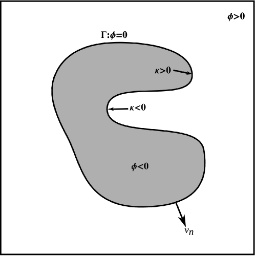
Fig. 1: An example level set domain with the interface $\Gamma$, interior $\phi<0$, exterior $\phi>0$ shown. The sign of the curvature, $\kappa$, and the interface normal velocity $v_{n}$, is also shown.

An implicit representation of the interface has the advantage of treating all topology changes naturally without any complex remeshing. Various geometric quantities such as the normal vector and curvature can be easily computed as

$$\boldsymbol{n}= \frac{\nabla\phi}{\left|\left|\nabla\phi\right|\right|},$$ (2)

$$\kappa= \nabla\cdot\frac{\nabla\phi}{\left|\left|\nabla\phi\right|\right|}.$$ (3)

The motion of the interface due to an underlying flow field $\boldsymbol{v}$ can be modelled by a standard advection equation,

$$\frac{\partial\phi}{\partial t}+\boldsymbol{v}\cdot\nabla\phi=0.$$ (4)

If the normal velocity on the interface is known the equivalent advection equation is

$$\frac{\partial\phi}{\partial t}+v_{n}\left|\left|\nabla\phi\right|\right|=0.$$ (5)

For accuracy reasons it is preferential to keep $\phi$ as a signed distance function such that $\left|\left|\nabla\phi\right|\right|=1$. In many situations Eq. 4 or Eq. 5 do not enforce this condition. A reinitialization process is typically used to retain the signed-distance property of $\phi$ by solving a secondary PDE in the form of [6]

$$\frac{\partial\phi}{\partial\tau}=\textrm{sign}(\phi_{0})\cdot(\left|\left|\nabla\phi\right|\right|-1),$$ (6)

where $\tau$ is a pseudo-time taken proportional to the grid spacing.

In many systems the motion of an interface is influenced by the curvature or the variation of the curvature (surface diffusion) along an interface [1, 7, 8, 9, 10, 11]. The dependence of the flow on the curvature causes numerical stability issues for many methods. Explicit schemes require small time steps, on the order of $h^{2}$ for curvature based flows and $h^{4}$ for surface diffusion, where $h$ is the grid spacing [12, 13] . These stringent restrictions lead to long computation times and can limit the size of the system that may be investigated. A fully implicit method would alleviate the time step restriction but would add the complexity of solving a possibly non-linear system every time step. Another approach is to extract the linear portion of the advection equation and treat it implicitly, with the non-linear part treated explicitly [14, 15]. This has the advantage of numerically stabilizing the system at the cost of a slight deterioration of the accuracy of the solution.

The gradient augmented level set method is an extension of the standard level set method which advances the level set and the gradient of the level set field [16]. This is accomplished by advecting the level set and its gradient as independent quantities in a coupled manner, ensuring that the relationship between the quantities remains. This additional information allows for the determination of data on a sub-grid level, allowing for the use of coarser meshes. The original gradient augmented level set method was demonstrated using analytic flow fields and demonstrated excellent accuracy with minimal additional computational cost. The use of the augmented gradient level set method in modelling vesicle motion [7] has shown that while the time step restriction is not as stringent as regular explicit schemes it is not possible to take time steps on the order of the grid spacing, as is possible with semi-implicit methods [14, 15].

In this article a semi-implicit gradient augmented level set (SIGALS) method is presented. This extension allows for the investigation of both mean curvature and surface diffusion based motions, with restrictions based on accuracy and not stability. The tracking of the level set gradient function provides more accuracy and alleviates some of the non-local behavior of the original semi-implicit level set method [15]. In Sec. 2 the standard gradient augmented method and the original semi-implicit method are briefly outlined. A description of the semi-implicit gradient augmented level set method follows. Convergence analysis for a simple case and sample results are presented in Sec. 3. Section 4 provides a short conclusion.

2 Development of the Method

This section will outline the standard semi-implicit level set scheme, the original augmented level set method, and the proposed new method. This section concludes by providing the complete algorithm of the proposed method.

2.1 The Semi Implicit Level Set Formulation

The level set advection equation, Eq. (4), can be written as a Hamilton-Jacobi equation,

$$\frac{\partial\phi}{\partial t}+H\left(\boldsymbol{x},t,\phi,\nabla\phi\right)=0.$$ (7)

A Hamilton-Jacobi equation can be made semi-implicit one of two ways. The first is to extract the linear portion of the Hamiltonian, $H$, and treat it implicitly,

$$\frac{\partial\phi}{\partial t}+L\left(\boldsymbol{x},t^{n+1},\phi^{n+1},\nabla\phi^{n+1}\right)+N\left(\boldsymbol{x},t^{n},\phi^{n},\nabla\phi^{n}\right)=0,$$ (8)

where $L$ is the linear portion and $N$ is the nonlinear portion such that $H=L+N$. If it is not possible to explicitly extract the linear portion one can always determine an approximation to the linear portion and solve the following semi-implicit equation,

$$\frac{\partial\phi}{\partial t}+H\left(\boldsymbol{x},t^{n},\phi^{n},\nabla\phi^{n}\right)+\widetilde{L}\left(\boldsymbol{x},t^{n},\phi^{n},\nabla\phi^{n}\right)-\widetilde{L}\left(\boldsymbol{x},t^{n+1},\phi^{n+1},\nabla\phi^{n+1}\right)=0,$$ (9)

where $\widetilde{L}$ is the approximate linear portion. For mean curvature based flows it is typical to take $\widetilde{L}=\beta\nabla^{2}\phi$ while for surface diffusion based flows $\widetilde{L}=\beta\nabla^{4}\phi$, where $\beta$ is a constant and typically taken to be $\beta=1/2$ [14, 15]. This additional smoothing allows the semi-implicit level set method to utilize much larger time steps than is possible with an explicit scheme [15]. For example, the motion by surface diffusion of a seven-lobed star requires a CFL condition of $\Delta t/h^{4}\approx 0.25$ using an explicit method [12] compared to a CFL condition of $\Delta t/h^{4}\approx 2\times 10^{4}$ for the semi-implicit scheme [15].

2.2 Standard Gradient Augmented Level Set Method

The gradient augmented level set method is an extension of the standard level set method which advects both the level set, $\phi$, and the level set gradient, $\boldsymbol{\psi}=\nabla\phi=\left(\phi_{x},\phi_{y},\phi_{z}\right)=\left(\psi^{x},\psi^{y},\psi^{z}\right)$:

$$\frac{\partial\phi}{\partial t}+\boldsymbol{v}\cdot\nabla\phi= 0,$$ (10)

$$\frac{\partial\boldsymbol{\psi}}{\partial t}+\boldsymbol{v}\cdot\nabla\boldsymbol{\psi}+\nabla\boldsymbol{v}\cdot\boldsymbol{\psi}= 0.$$ (11)

The inclusion of gradient information allows for the determination of sub-grid information. Take as an example two grid points, $x_{0}=0$ and $x_{1}=1$, on a one dimensional grid with $\phi\left(x_{0}\right)=\phi\left(x_{1}\right)=0.1$ with $\phi_{x}\left(x_{0}\right)=1$ and $\phi_{x}\left(x_{1}\right)=-1$. The exact level set, the signed distance function, gives an interface ($\phi=0$) at points $x=0.1\textrm{ and }0.9$. Using only the level set values linear interpolation does not return any interface points in this domain. The additional gradient information allows for the determination of a Hermite interpolant giving interface locations of $x\approx 0.112$ and $x\approx 0.887$. See Fig. 2 for a graphical representation.

Fig. 2: A one-dimensional grid with data provided at grid points $x=0$ and $x=1$. The linear interpolant misses the interface existing between the two grid points. The Hermite interpolant determined using the additional gradient information finds two interfaces close to the true interface locations.

To ensure that the level set and gradient field remain coupled throughout time Eqs. (10) and (11) are advanced in a coherent and fully coupled manner [16]. Lagrangian techniques are used to trace characteristics back in time to determine departure locations. Using the available information a Hermite interpolating polynomial is calculated and utilized to determine the departure values for the level set and gradient functions. To first order this results in the following scheme,

$$\boldsymbol{x}_{d} =\boldsymbol{x}-\Delta t\;\boldsymbol{v}\left(\boldsymbol{x},t\right),$$ (12)

$$\nabla{\boldsymbol{x}}_{d} =\boldsymbol{I}-\Delta t\;\nabla\boldsymbol{v}\left(\boldsymbol{x},t\right),$$ (13)

$$\phi\left(\boldsymbol{x},t\right) =P\left(\boldsymbol{x}_{d},t-\Delta t\right),$$ (14)

$$\boldsymbol{\psi}\left(\boldsymbol{x},t\right) =\nabla{\boldsymbol{x}}_{d}\cdot\boldsymbol{G}\left(\boldsymbol{x}_{d},t-\Delta t\right),$$ (15)

where $P(\boldsymbol{x},t)$ is the Hermite interpolating polynomial of $\phi$ at a time $t$, $\boldsymbol{G}=\nabla P$ is the gradient of the Hermite interpolant defined for the level set, while $\boldsymbol{x}_{d}$ and $\nabla{\boldsymbol{x}}_{d}$ are the departure location and “departure” gradient, respectively. Implementing a third-order version of the method Nave et. al. demonstrated that for analytic flow fields the gradient augmented provides results comparable to higher-order WENO schemes at a lower computational cost [16]. Results for flows depending on derivatives of the level set function where not presented.

2.3 The Semi-Implicit Gradient Augmented Level Set Method

The semi-implicit gradient augmented level set method is a combination of the methods briefly explained in Secs. 2.1 and 2.2. The goal is to combine the additional accuracy afforded by explicitly tracking gradient information with the stability properties of a semi-implicit scheme. Equations (10) and (11) are replaced with

$$\frac{D\phi}{Dt}+\beta L\phi-\beta L\phi =0,$$ (16)

$$\frac{D\boldsymbol{\psi}}{Dt}+\nabla\boldsymbol{v}\cdot\boldsymbol{\psi}+\beta L\boldsymbol{\psi}-\beta L\boldsymbol{\psi} =0,$$ (17)

where $D/Dt$ is the material (Lagrangian) derivative, $L$ is a linear operator, and $\beta$ is a constant. To first-order in time this can be written as

$$\boldsymbol{x}_{d} =\boldsymbol{x}-\Delta t\;\boldsymbol{v}\left(\boldsymbol{x},t\right),$$ (18)

$$\nabla{\boldsymbol{x}}_{d} =\boldsymbol{I}-\Delta t\;\nabla\boldsymbol{v}\left(\boldsymbol{x},t\right),$$ (19)

$$\widetilde{\phi} =P\left(\boldsymbol{x}_{d},t-\Delta t\right),$$ (20)

$$\widetilde{\boldsymbol{\psi}} =\nabla{\boldsymbol{x}}_{d}\cdot\boldsymbol{G}\left(\boldsymbol{x}_{d},t-\Delta t\right),$$ (21)

$$\frac{\phi_{n+1}-\widetilde{\phi}}{\Delta t} =\beta L\phi_{n+1}-\beta L\phi_{n},$$ (22)

$$\frac{\boldsymbol{\psi}_{n+1}-\widetilde{\boldsymbol{\psi}}}{\Delta t} =\beta L\boldsymbol{\psi}_{n+1}-\beta L\boldsymbol{\psi}_{n},$$ (23)

The linear operator $L$ is based on the underlying flow field. For mean curvature flow $L=\nabla^{2}$ while for surface diffusion $L=\nabla^{4}$. If $\beta=0$ the method results in the standard gradient augmented method. If instead of Eqs. 18 to 21 values are set as $\widetilde{\phi}=\phi_{n}$ and $\widetilde{\boldsymbol{\psi}}=\boldsymbol{\psi}_{n}$ the method results in the standard semi-implicit level set scheme.

The location $\boldsymbol{x}_{d}$ is obtained by tracing characteristics backwards in time. In general this location will not lie on a grid point and thus the use of an interpolant, $P$ and $\boldsymbol{G}=\nabla P$, is required. In two dimensions let $\boldsymbol{x}_{d}$ lie within a grid cell $\Omega_{i,j}$ enclosing the region given by four grid points: $\boldsymbol{x}_{i,j}$, $\boldsymbol{x}_{i+1,j}$, $\boldsymbol{x}_{i,j+1}$, and $\boldsymbol{x}_{i+1,j+1}$. Using the value of level set, $\phi$, and gradient field, $\boldsymbol{\psi}=(\psi^{x},\psi^{y})$, at time $t-\Delta t$ it is possible to define the Hermite interpolant over the grid cell by requiring that $P(\boldsymbol{x}_{m,n})=\phi_{m,n}$, $\partial_{x}P(\boldsymbol{x}_{m,n})=\psi^{x}_{m,n}$, $\partial_{y}P(\boldsymbol{x}_{m,n})=\psi^{y}_{m,n}$, and $\partial_{xy}P(\boldsymbol{x}_{m,n})=(\partial_{x}\psi^{y}_{m,n}+\partial_{y}\psi^{x}_{m,n})/2$ for $m={i,i+1}$ and $n={j,j+1}$. The gradient interpolant is then defined as $\boldsymbol{G}=\nabla P$.

Two velocity fields are considered here. The first velocity field is mean curvature flow given by $v_{n}=-\kappa$ or $\boldsymbol{v}=-\kappa\boldsymbol{n}$, where $\kappa$ is the mean curvature and $\boldsymbol{n}$ is the unit normal vector. The unit normal vector is simply given as the normalized gradient vector:

$$\boldsymbol{n}=\frac{\boldsymbol{\psi}}{\|\boldsymbol{\psi}\|}.$$ (24)

The curvature is computed as

$$\kappa=\frac{\phi_{xx}\phi_{y}^{2}+\phi_{yy}\phi_{x}^{2}-2\phi_{xy}\phi_{x}\phi_{y}}{\left(\phi_{x}^{2}+\phi_{y}^{2}+\epsilon\right)^{3/2}}$$ (25)

for two-dimensional flows and

$$\kappa= (\phi_{xx}\left(\phi_{y}^{2}+\phi_{z}^{2}\right)+\phi_{yy}\left(\phi_{x}^{2}+\phi_{z}^{2}\right)+\phi_{zz}\left(\phi_{x}^{2}+\phi_{y}^{2}\right)$$

$$-2\phi_{xy}\phi_{x}\phi_{y}-2\phi_{xz}\phi_{x}\phi_{x}-2\phi_{yz}\phi_{y}\phi_{z})/\left(\phi_{x}^{2}+\phi_{y}^{2}+\phi_{z}^{2}+\epsilon\right)^{3/2}$$ (26)

for three-dimensional flows. In the above the first-order derivatives, $\phi_{x}$, $\phi_{y}$, and $\phi_{z}$ are replaced by their corresponding values in the $\boldsymbol{\psi}$ vector. The second-order derivatives are obtained by first derivatives of the $\boldsymbol{\psi}$ vector. Any cross derivatives are averages of the two possible first derivatives of the gradient vector, i.e. $\phi_{xy}=(\partial_{x}\psi^{y}+\partial_{y}\psi^{x})/2$. The value $\epsilon=10^{-8}$ is added to ensure that no division by zero will occur.

The second velocity field considered is that of surface diffusion, given by $v_{n}=\nabla^{2}_{s}\kappa$ or $\boldsymbol{v}=\left(\nabla^{2}_{s}\kappa\right)\boldsymbol{n}$ where $\nabla^{2}_{s}$ is the surface Laplacian. Assume that the curvature is known in the vicinity of the interface. In two dimensions the surface Laplacian of the curvature can then be calculated as

$$S=\nabla_{s}^{2}\kappa=\frac{\kappa_{xx}\phi_{y}^{2}+\kappa_{yy}\phi_{x}^{2}-2\kappa_{xy}\phi_{x}\phi_{y}}{\phi_{x}^{2}+\phi_{y}^{2}+\epsilon}-\kappa\frac{\kappa_{x}\phi_{x}+\kappa_{y}\phi_{y}}{\sqrt{\phi_{x}^{2}+\phi_{y}^{2}+\epsilon}},$$ (27)

while for the three-dimensional case

$$S=\nabla_{s}^{2}\kappa= (\kappa_{xx}\left(\phi_{y}^{2}+\phi_{z}^{2}\right)+\kappa_{yy}\left(\phi_{x}^{2}+\phi_{z}^{2}\right)+\kappa_{zz}\left(\phi_{x}^{2}+\phi_{y}^{2}\right)$$

$$-2\kappa_{xy}\phi_{x}\phi_{y}-2\kappa_{xz}\phi_{x}\phi_{z}-2\kappa_{yz}\phi_{y}\phi_{z})/(\phi_{x}^{2}+\phi_{y}^{2}+\phi_{z}^{2}+\epsilon)$$

$$-\kappa(\kappa_{x}\phi_{x}+\kappa_{y}\phi_{y}+\kappa_{z}\phi_{z})/\sqrt{\phi_{x}^{2}+\phi_{y}^{2}+\epsilon}.$$ (28)

The curvature and surface diffusion velocity fields defined above are only defined on the interface. To determine a smooth velocity field elsewhere in the domain values can be extended from the interface through the use of an extension equation applied to a quantity $q$ [14, 15, 17],

$$\frac{\partial q}{\partial\tau}+\textrm{sign}(\phi)\boldsymbol{n}\cdot\nabla q=0,$$ (29)

where $\tau$ is a fictitious time.

The semi-implicit gradient augmented level set scheme can be summarized in the following two algorithms:

Algorithm 1 Compute the Velocity Field

0:  $\phi$ and $\boldsymbol{\psi}$

  Set $\kappa=0$ in the entire domain.

  Compute $\kappa$ using either Eq. (25) or (2.3) at grid points next to the interface.

  Extend $\kappa$ by at least 4 grid points using an extension algorithm [14, 15, 17].

  if velocity field is surface diffusion then

     Set $S=0$ in the entire domain.

     Compute $S$ using either Eq. (27) or (2.3) at grid points next to the interface.

     Extend $S$ by at least 4 grid points using an extension algorithm [14, 15, 17].

     Set the velocity as $\boldsymbol{v}=S\boldsymbol{n}$.

  else

     Set the velocity as $\boldsymbol{v}=-\kappa\boldsymbol{n}$.

  end if

  return  $\boldsymbol{v}$

Algorithm 2 Advance the Level Set and Gradient Fields

0:  $\phi_{n}$ and $\boldsymbol{\psi}_{n}$.

  Compute $\boldsymbol{v}$ using Algorithm 1.

  for every grid point in the domain do

     Compute the departure point $\boldsymbol{x}_{d}$ using Eq. 18.

     Compute the departure gradient $\nabla\boldsymbol{x}_{d}$ using Eq. 19

     Evaluate the tentative Lagrangian solutions $\widetilde{\phi}$ and $\widetilde{\boldsymbol{\psi}}$ by Eqs. (20) and (21).

  end for

  if velocity field is surface diffusion then

     Set $L=\nabla^{4}$

  else

     Set $L=\nabla^{2}$

  end if

  Solve $\left(\boldsymbol{I}-\Delta t\beta L\right)\phi_{n+1}=\widetilde{\phi}-\Delta t\beta L\phi_{n}$.

  Solve $\left(\boldsymbol{I}-\Delta t\beta L\right)\boldsymbol{\psi}_{n+1}=\widetilde{\boldsymbol{\psi}}-\Delta t\beta L\boldsymbol{\psi}_{n}$.

  return  $\phi_{n+1}$ and $\boldsymbol{\psi}_{n+1}$.

3 Numerical Results

To avoid any anisotropy introduced by the use of center finite difference approximations all derivatives will be approximated by isotropic finite differences [18]. The linear systems in Eqs. (22) and (23) are solved using a standard Bi-CGSTAB method [19, 20]. All of the results will be first order in time and utilize second-order isotropic finite differences. In each case periodic boundary conditions are assumed and a constant of $\beta=0.5$ is used. The curvature and surface Laplacian of curvature are first calculated near the interface and then extended to the rest of the domain, as shown in the Alg. 1. The time step is given by $\Delta t$ while the uniform grid spacing is given by $h$. Every initial interface is initially described by a signed distance function. Please note that no level set reinitialization was performed during the simulations.

3.1 Mean Curvature Flow

Here the evolution of two- and three-dimensional interfaces under mean-curvature flow will be shown. For all cases in this section the velocity of the interface is given by $\boldsymbol{v}=-\kappa\boldsymbol{n}$.

First consider a circular interface. With mean curvature flow a circular interface beginning with an initial radius of $r_{0}$ will collapse uniformly. A sample result is presented in Fig. 3 for a grid spacing of $h=0.0625$ and a time step of $\Delta t=4h^{2}=0.015625$.

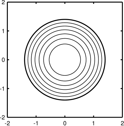
Fig. 3: A circle collapsing due to mean curvature flow. The initial interface is represented by the thick line. The the grid spacing is $h=0.0625$ and the time step is $\Delta t=4h^{2}=0.015625$. The interface is shown in time increments of $10\Delta t$.

The collapse of a circular interface under mean curvature flow is a situation with a known analytic solution and thus allows for the investigation of the accuracy of the SIGALS scheme. At time $t$ the radius of the circle is given by

$$r(t)=\sqrt{r_{0}^{2}-2t},$$ (30)

where $r_{0}$ is the initial radius. The interface was allowed to evolve until a time of $t=0.375$ with various grid spacings and a time step set to $\Delta t=8h^{2}$. The level set and gradient field values for grid points next to the interface are compared to a signed distance function describing a circle with the radius given in Eq. (30). The resulting errors are shown in Tables 1 and 2. The level set retains the second-order in space accuracy of the underlying discretization while the gradient is one-half order lower.

Table 1: Level set error for a circle with $v_{n}=-\kappa$ using $\Delta t=8h^{2}$.

N	$h$	$L_{2}$	Order	$L_{\infty}$	Order
64	0.0625	$2.60\times 10^{-3}$		$4.23\times 10^{-2}$
128	0.03125	$6.47\times 10^{-4}$	2.0	$1.37\times 10^{-2}$	1.63
256	0.015625	$1.64\times 10^{-4}$	1.98	$4.8\times 10^{-3}$	1.51
512	0.0078125	$4.20\times 10^{-5}$	1.96	$1.61\times 10^{-3}$	1.58

Table 2: Gradient error for a circle with $v_{n}=-\kappa$ using $\Delta t=8h^{2}$.

N	$h$	$L_{2}$	Order	$L_{\infty}$	Order
64	0.0625	$6\times 10^{-4}$		$1.21\times 10^{-2}$
128	0.03125	$1.68\times 10^{-4}$	1.84	$3.7\times 10^{-3}$	1.71
256	0.015625	$5.64\times 10^{-5}$	1.57	$1.7\times 10^{-3}$	1.12
512	0.0078125	$2.01\times 10^{-5}$	1.49	$8.2\times 10^{-4}$	1.05

Similar behavior is observed in more complex interfaces. The collapse of a Cassini oval is shown in Fig. 4. Initially the interface has regions of both positive and negative curvature. The positive curvature regions move towards the center of the domain while those with negative curvature move away from the center. After some time an ellipse-like interface is obtained. From this point forward the interface collapses to a point.

Fig. 4: Motion by mean curvature for a Cassini oval at different times on a $128\times 128$ grid. The grid spacing is $h=0.03125$ while the time step is $\Delta t=0.03$. The thick line represents the initial interface while the arrow indicates the direction of motion. Subsequent interface locations are shown in time increments of $3\Delta t$. Eventually the interface will collapse to a point.

Similar results are seen for a two-dimensional four-lobe star, Fig. 5. The interface evolves until the curvature is strictly positive at which point the shape collapses to a point.

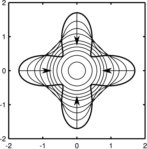
Fig. 5: Evolution of a 4-lobe star under mean curvature flow. The grid size $256\times 256$ giving a grid spacing of $h=0.015625$. The time step is $\Delta t=0.005$. The thick line is the initial interface with subsequent interface locations shown in increments of $20\Delta t$. The arrows indicate the direction of motion.

To demonstrate the added stability properties of the SIGALS scheme as compared to the original gradient augmented level set method the evolution of a five-lobe star is shown in Fig. 6. A common grid spacing of $h=0.03125$ and time step $\Delta t=5\times 10^{-4}$ is used for both cases. This results in a CFL condition of $\Delta t/h^{2}\approx 0.5$. Over time the standard gradient augmented method begins to demonstrate numerical instabilities. The SIGALS method does not demonstrate any instability and shows the expected behavior.

Standard Gradient Augmented Level Set Method

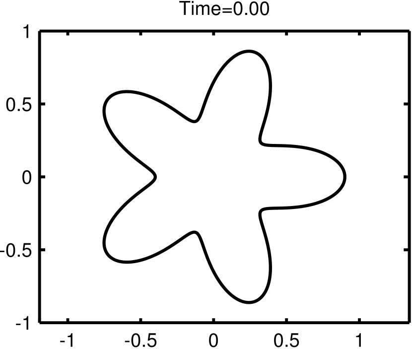
Semi-Implicit Gradient Augmented Level Set Method

Fig. 6: A comparison of the standard gradient augmented level set method with the semi-implicit augmented method using the same time step for both methods. The five-lobe star is collapsing under mean curvature flow, $v_{n}=-\kappa$, for $\Delta t=5\times 10^{-4}$ and $h=0.03125$ giving $\Delta t/h^{2}\approx 0.5$. The full domain is the region given by $[-2,2]^{2}$

The extension of the SIGALS method to three dimensions is demonstrated in Fig. 7, which shows the collapse of a three-dimensional Cassini oval with mean-curvature flow. Due to the additional curvature the neck region does not thicken as in the two-dimensional Cassini oval case, instead the surface collapses with the surface splitting into two separate interfaces. This result clearly demonstrates the level sets ability to handle topological changes naturally.

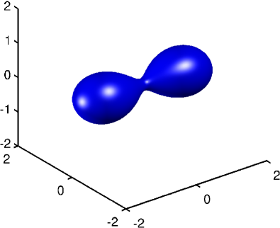
(a) $t=0$

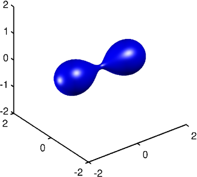
(b) $t=0.025$

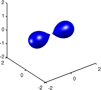
(c) $t=0.04$

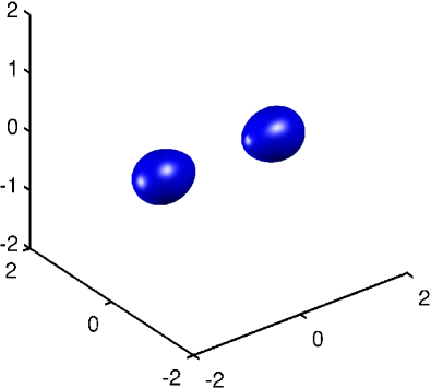
(d) $t=0.075$

Fig. 7: Collapse of a three dimensional Cassini oval under mean curvature flow for $h=0.0625$ and $\Delta t=0.005$.

3.2 Surface Diffusion

This section considers the motion of interfaces due to the intrinsic variation of the curvature along the interface, or simply called surface diffusion. In this case the velocity of an interface is given by $\boldsymbol{v}=\left(\nabla_{s}^{2}\kappa\right)\boldsymbol{n}$, where $\nabla_{s}^{2}$ is the surface Laplacian. The final result for all surface diffusion cases will be a constant curvature interface: a circle in two dimensions and a sphere in three dimensions.

The first shape considered is that of an inclined ellipse, Fig. 8. As expected the ellipse smoothly transitions to the circular interface. This interface is also utilized as a qualitative check on the spatial and temporal convergence of the method. The grid study is performed by fixing the time step at $\Delta t=10^{-4}$ and varying the grid spacing. The temporal study fixes the grid size at $\Delta x=0.0312$ and varies the time step. The results for a time of 0.1 are seen in Fig. 9 and demonstrate the method quickly converging to a common solution.

Fig. 8: Motion by surface diffusion for an elliptical interface for a grid spacing of $h=0.03125$ and a time step of $\Delta t=0.001\approx 1048\Delta x^{4}$. The thick line is the initial interface and the arrows indicate the direction of motion. Interfaces are shown for times of 0, 0.05, 0.2, and 0.6.

(a) Spatial Study

(b) Time Study

Fig. 9: Qualitative convergence check for motion due to surface diffusion. For the spatial study the time step is fixed at $\Delta t=10^{-4}$ while for the time study the grid spacing is fixed at $h=0.015625$. All results are shown at a time of $t=0.1$.

The evolution of a five-lobed star under surface diffusion is seen in Fig. 10. In addition to the location of the interface over time the total enclosed area and interfacial length are also presented. It is clear that the enclosed area remains constant at $\pi$ and the interface length is minimized to a value of $2\pi$.

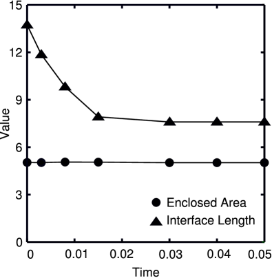
Fig. 10: Motion by surface diffusion for a five-lobe star at using a grid spacing $\Delta x=0.0625$ and a time step $\Delta t=0.001\approx 65\Delta x^{4}$. The motion of the interface is seen in (a) while the enclosed area and interface length are tracked in (b).

Next consider two three-dimensional surfaces, a dumbbell surface, Fig. 11, and a more complicated box-like surface, Fig. 12. The dumbbell results in two distinct spheres due to the pinching-off of the thin region while the more complicated box-like surface results in a single sphere.

(a) $t=0$

(b) $t=0.0003$

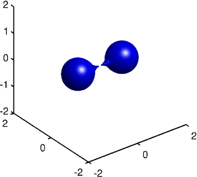
(c) $t=0.0005$

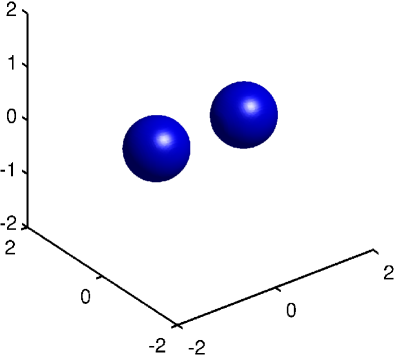
(d) $t=0.005$

Fig. 11: Motion by surface diffusion for a three-dimensional dumbbell surface. The grid spacing is $h=0.0625$ and the time step is $\Delta t=0.0001$

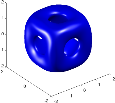
(a) $t=0$

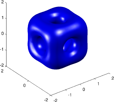
(b) $t=0.05$

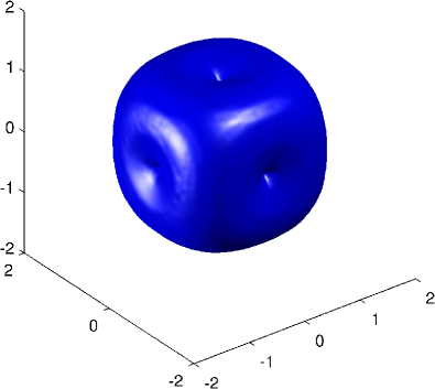
(c) $t=0.09$

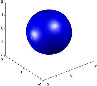
(d) $t=0.3$

Fig. 12: Evolution of a complex three-dimensional shape under surface diffusion. The grid spacing is $h=0.0625$ and the time step is $\Delta t=10^{-4}$

Finally consider the merging of a circle and ellipse under surface diffusion, Fig. 13. The circle should remain stationary until the evolving ellipse contacts it. In the original semi-implicit level set work it was demonstrated that the non-local nature of the smoothing operator results in slight perturbation of the interfaces [15]. In this work a similar result is noticed but to a smaller degree than in the standard semi-implicit scheme. This is further demonstrated in Fig. 14, where a comparison between the standard semi-implicit level set solution, the SIGALS method, and the reference solution is shown for times of $t=0.0235$ and $t=0.025$. The reference solution was obtained by evolving the interfaces independently. While both the regular and gradient-augmented semi-implicit level set schemes appear to be working correctly at a time of $t=0.0235$, Fig. 14(a), the standard semi-implicit scheme clearly demonstrates incorrect behavior at time $t=0.025$, Fig. 14(b). This is due to large oscillations in the calculated curvature, shown in Figs. 14(c) and 14(d) for the circle and ellipse interfaces, respectively, at the time $t=0.0235$. While oscillations still occur in the SIGALS method they are smaller than in standard method. This is due to the additional information provided by explicitly tracking the gradient of the level set.

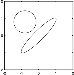
(a) $t=0$

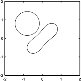
(b) $t=0.01$

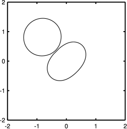
(c) $t=0.029$

(d) $t=0.0304$

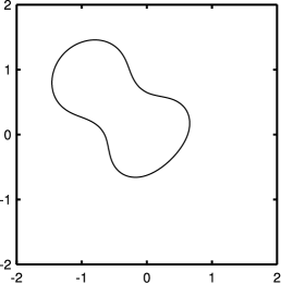
(e) $t=0.032$

(f) $t=0.035$

Fig. 13: Coalescence of two bodies under surface diffusion flow. The time step is $\Delta t=0.0001$ and while the grid spacing is $h=0.03125$. There is minimal spurious motion of the circle before merging.

(a) $t=0.0235$

(b) $t=0.025$

(c) Circle

(d) Ellipse

Fig. 14: A comparison between the standard semi-implicit level set, the SIGALS method, and the reference solution for the case of a merging circle and ellipse. Two representative times are shown in (a) and (b). The curvature along the (c) circle and (d) ellipse are also shown for a time of $t=0.0235$. The large curvature oscillations in the standard semi-implicit level set result in the incorrect behavior observed in (b).

4 Summary

This work represents a combination of the standard semi-implicit level set method and the gradient-augmented level set method. The result is a hybrid Lagrangian-Eulerian method that is easily applied in both two- and three-dimensions. Sample results were provided for motion by mean curvature and surface diffusion. The addition of gradient information reduced the non-local nature of the semi-implicit scheme and allowed for investigations of flows depending on high-order derivatives of the interface.

References

- [1] Z. Li, H. Zhao, H. Gao, A numerical study of electro-migration voiding by evolving level set functions on a fixed Cartesian grid, Journal of Computational Physics 152 (1999) 281–304.
- [2] J. Luo, Z. Luo, L. Chen, L. Tong, M. Wang, A semi-implicit level set method for structural shape and topology optimization, Journal of Computational Physics 227 (11) (2008) 5561–5581.
- [3] R. Malladi, J. Sethian, Image processing via level set curvature flow., Proceedings of the National Academy of Sciences of the United States of America 92 (15) (1995) 7046–50.
- [4] J. A. Sethian, P. Smereka, Level Set Methods for Fluid Interfaces, Annual Review of Fluid Mechanics 35 (1) (2003) 341–372.
- [5] S. Osher, J. Sethian, Fronts propagating with curvature-dependent speed - algorithms based on hamilton-jacobi formulations, Journal of Computational Physics 79 (1) (1988) 12–49.
- [6] M. Sussman, A Level Set Approach for Computing Solutions to Incompressible Two-Phase Flow (Sep. 1994).
- [7] D. Salac, M. Miksis, A level set projection model of lipid vesicles in general flows, Journal of Computational Physics 230 (22) (2011) 8192 – 8215.
- [8] D. Adalsteinsson, J. Sethian, A level set approach to a unified model for etching, deposition, and lithography .3. Redeposition, reemission, surface diffusion, and complex simulations, Journal of Computational Physics 138 (197) 193–223.
- [9] B. Merriman, J. Bence, S. Osher, Motion of multple junctions - a level set approach, Journal of Computational Physics 112 (1994) 334–363.
- [10] W. W. Mullins, Theory of thermal grooving, Journal of Applied Physics 28 (3) (1957) 333–339.
- [11] S. Veerapaneni, D. Gueyffier, D. Zorin, G. Biros, A boundary integral method for simulating the dynamics of inextensible vesicles suspended in a viscous fluid in 2d, Journal of Computational Physics 228 (7) (2009) 2334–2353.
- [12] D. Chopp, J. Sethian, Motion by Intrinsic Laplacian of Curvature, Interfaces and Free Boundaries 1 (1999) 1–18.
- [13] M. Khenner, A. Averbuch, M. Israeli, M. Nathan, Numerical Simulation of Grain Boundary Grooving By Level Set Method , Journal of Computational Physics (2001) 764–784.
- [14] D. Salac, W. Lu, A Local Semi-Implicit Level-Set Method for Interface Motion, Journal of Scientific Computing 35 (2-3) (2008) 330–349.
- [15] P. Smereka, Semi-implicit level set methods for curvature and surface diffusion motion, Journal of Scientific Computing 19 (2003) 439–456.
- [16] J.-C. Nave, R. R. Rosales, B. Seibold, A gradient-augmented level set method with an optimally local, coherent advection scheme (May 2010).
- [17] D. Peng, A PDE-Based Fast Local Level Set Method, Journal of Computational Physics 155 (2) (1999) 410–438.
- [18] A. Kumar, Isotropic finite-differences, Journal of Computational Physics 201 (1) (2004) 109–118.
- [19] H. A. van der Vorst, Bi-cgstab: A fast and smoothly converging variant of bi-cg for the solution of nonsymmetric linear systems, SIAM Journal on Scientific Computing 13 (2) (1992) 631–644.
- [20] Y. Saad, Iterative Methods for Sparse Linear Systems, Second Edition, 2nd Edition, Society for Industrial and Applied Mathematics, 2003.