Understanding agent-based models of financial markets: a bottom-up approach based on order parameters and phase diagrams
Abstract
We describe a bottom-up framework, based on the identification of appropriate order parameters and determination of phase diagrams, for understanding progressively refined agent-based models and simulations of financial markets. We illustrate this framework by starting with a deterministic toy model, whereby independent traders buy and sell stocks through an order book that acts as a clearing house. The price of a stock increases whenever it is bought and decreases whenever it is sold. Price changes are updated by the order book before the next transaction takes place. In this deterministic model, all traders based their buy decisions on a call utility function, and all their sell decisions on a put utility function. We then make the agent-based model more realistic, by either having a fraction of traders buy a random stock on offer, or a fraction of traders sell a random stock in their portfolio. Based on our simulations, we find that it is possible to identify useful order parameters from the steady-state price distributions of all three models. Using these order parameters as a guide, we find three phases: (i) the dead market; (ii) the boom market; and (iii) the jammed market in the the phase diagram of the deterministic model. Comparing the phase diagrams of the stochastic models against that of the deterministic model, we realize that the primary effect of stochasticity is to eliminate the dead market phase.
keywords:
Financial markets , agent-based models , order parameters , phase diagramPACS:
89.65.Gh1 Motivation
Economies and financial markets are complex systems described by a large number of variables, which are in turn influenced by an even larger number of factors or players. To understand how these complex systems evolve in time, an approach that has been very fruitful thus far is to consider the dynamics of a small number of aggregate collections of homogeneous variables. In this approach, the dependences of aggregate averages on other aggregate averages, and on time, are modeled by coupled systems of ordinary or partial differential equations. While this equation-based approach has been able to provide rigorous theorems, and generate much economic insights, it is fundamentally mean field in character, in that variances and higher-order statistical moments of the aggregates are assumed to be slaves of the averages, and have no independent dynamics of their own. In many important and interesting situations in the real world, this assumption is indeed valid, because the number of variables in each homogeneous aggregate is large, and the central limit theorem applies.
However, in many other interesting real-world situations, statistical fluctuations can become an important driver in the time evolution of economies and financial markets. When this happens, the variances and higher statistical moments of the aggregates become large, and their dynamics cannot be deduced from those of the averages alone. This is where agent-based models and simulations become invaluable as a tool for understanding the dynamics of the economic or financial system as a whole. Since the pioneering work of Arthur and co-workers [1], there has been rapidly growing interest in the use of agent-based simulations as a computational platform for performing ‘controlled experiments’ in an economic setting [2, 3, 4]. This has culminated in several reviews [5, 6, 7] and monographs [8, 9, 10] on the subject. In general, economists have taken a top-down approach to agent-based modeling, implementing neo-classical economic axioms, which are then systematically relaxed to incorporate the effects of heterogenuity [11, 12], long-term memory [13], and learning [14]. While this line of agent-based research has been able to give stylized and qualitative results, it is generally very difficult to draw quantitative, and deeper inferences and insights, because of large statistical fluctuations within the simulations.
In contrast, highly simplified models have been the choice of physicists [15, 16, 17, 18, 19, 20, 21], because such models are easy to understand in quantitative terms. In this paper, we propose a bottom-up framework for going between the two agent-based modeling approaches. We start by describing in Section 2 a highly simplistic agent-based model, whose purpose is to illustrate the ideas behind the model differentiation framework, rather than to accurately describe the real world. After working out its phase diagram in Section 3, we refine the model by introducing a stochastic component in the trading strategies of the agents. By examining how the phase diagram is modified by the additional rules, we report insights gained from our preliminary study. In Section 5, we discuss how we can refine the model progressively to make its dynamics more and more realistic, and ultimately develop a picture on the hierarchy of complexities that emerge at various levels of realism in the models. Our goal is to eventually be able to identify robust market behaviours, which depend on the gross structure of the models but not the details, and also fragile market behaviours, which depends sensitively on certain model details, and hence are expected to appear only rarely in the real world.
2 Deterministic Model
To illustrate the basic framework in our bottom-up approach to understanding agent-based models, we start from a highly simplified model of a financial market, which consists of traders, stocks, and an order book. At the start of each simulation, we assign each of the stocks a random price , and a zero initial price change . A random initial offer for each stock is also made available on the order book, which plays the role of a clearing house. We then assign to each of the traders a random initial capital , as well as a random portfolio that excludes short positions. In this simple model, we assume that the traders do not directly interact with each other, but carry out transactions only through the order book. At each time step, the traders will trade in a randomized sequence. Each trader will buy one stock offered by the order book, and then sell one stock in his or her portfolio.
When it is trader ’s turn to trade, he or she will evaluate the utilities of the stocks on offer in the order book, based on the call function
| (1) |
where is the price of stock , and is the last price change of stock . Trader then buys however many units he or she can afford of the stock having the maximum utility. After this transaction, the order book increases the price of stock by one unit, and sets . Once this price adjustment is completed, trader evaluate the utilities of all stocks, using the put function
| (2) |
If stock is found to have the maximum utility, trader will sell all of stock in his or her portfolio. The order book then decreases the price of stock by one unit, and sets before the next trader trades.
In this model, we introduce two utility functions and to accommodate potential asymmetry between seller and buyer trading strategies. In these two utility functions, we also attempt to incorporate both fundamentalist and chartist tendencies. Given two stocks in the order book with the same positive long-term ratings, we expect fundamentalist traders to always buy the cheaper of the two. This tendency is accounted for in the call function by the price term , which decreases with increasing price . Chartist traders, on the other hand, will only buy an appreciating stock. Hence our choice of the price change term in the call function. We also assume that stocks are merely tools to increase capital assets, and traders attach no further value to them. Therefore, for the purpose of generating cash flow, we expect a fundamentalist trader will always sell his or her most expensive stock. This tendency is modeled by the price term in the put function. A chartist trader, whose trading decisions are based entirely on price changes, will only sell depreciating stocks. Hence our choice of the price change term in the put function. The traders in our simulations, who have no memory (and thus no capacity to learn), exhibit these fundamentalist and chartist tendencies to different extents, depending on the two independent parameters and . We vary and to determine the phase diagram of this model, whereby all traders behave rationally, and based their trading decisions on two deterministic utility functions.
3 Order Parameters and Phase Diagram
All our simulations were done with , , , , and . We chose these fixed parameters so that our system of agents resemble, at a very gross level, small markets like the Singapore Exchange (SGX), on which fewer than a thousand stocks are listed, attracting about 10,000 active traders. Assuming price movements are quantized on the level of S$0.05, the maximum stock price that we used to generate the initial distribution of stock prices, as well as the capital each trader is initially endowed with, both corresponds to an actual level of S$5.00. Our simulated market is thus a penny-stock market initially, played only by retail traders.
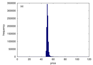
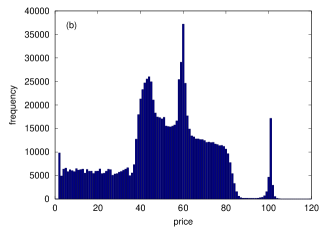
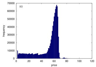
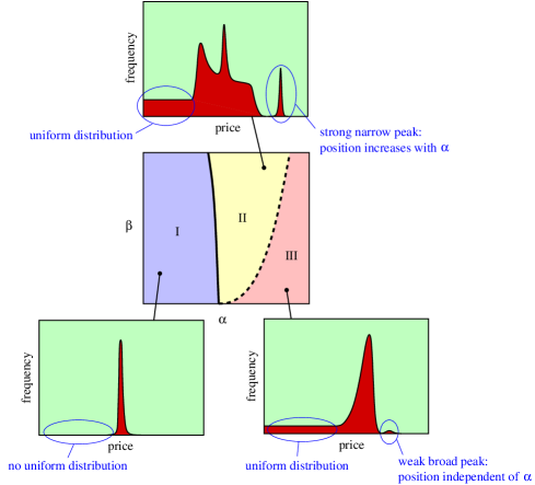
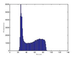
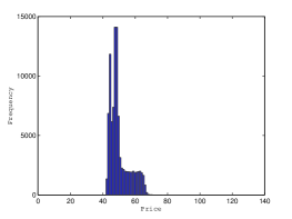
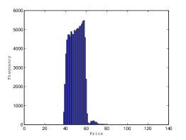
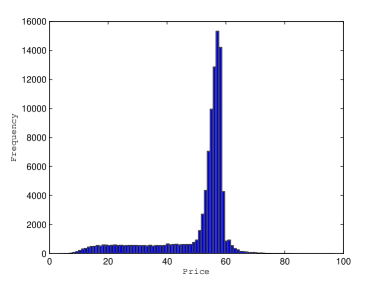
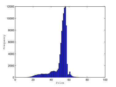
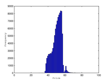
We ran each simulation up to 100 time steps, and examine the distribution of prices within all stocks. We find that for most parameter values , the initial uniform distribution of prices evolves into a steady-state distribution within 5–10 time steps. After a thorough examination of a large region of the - parameter space, we identified two robust features in the steady-state price distribution: (i) a uniform sub-distribution of below-average stock prices; and (ii) a gaussian sub-distribution of above-average stock prices. Based on features of these two sub-distributions, we identify three phases, I, II and III, for the deterministic model. In Figure 1, we show typical price distributions in phases I, II, and III. In phase I (Figure 1(a)), the steady-state price distribution is very narrowly distributed about . Both the uniform sub-distribution of below-average prices and the gaussian sub-distribution of above-average prices are absent. The uniform sub-distribution of below-average prices can be found in phases II (Figure 1(b)) and III (Figure 1(c)), which are distinguished by the gaussian sub-distribution of above-average prices. In phase II, this gaussian sub-distribution is strong and narrow, with a peak position that increases with , whereas in phase III, this gaussian sub-distribution is weak and broad, with a peak position that is independent of .
Our exploration of the - parameter space led us to sketch the phase diagram shown in Figure 2. Since our toy model is not intended to be a realistic model of any financial market, there is no real need to understand the phase diagram in detail. Nevertheless, the steady-state price distribution in Phase I is easy to understand: the buying of cheap stocks drive their prices up, and the selling of expensive stocks drive their prices down. This trading dynamics, which is essentially anti-diffusion in nature, eventually produces the sharp gaussian peak seen in the Phase I steady-state price distribution. We call Phase I a dead market, because there is very little trading activity in the steady state. While we do not understand all the features in the steady-state price distributions of Phases II and III, we do realize that in Phase II, traders can get increasing returns by ‘latching’ on to the sub-distribution of above-average stock prices. We therefore call this phase the boom market. In Phase III, this sub-distribution of above-average stock prices does not move as we increase , and so we call this phase the jammed market.
Now, the idea of studying phase transitions in economic systems is not new. LeBaron and co-workers recognize the existence of distinct economic phases from their early work on agent-based modeling [14]. More recently, Giardina and co-workers sketched the phase diagram of a sophisticated agent-based model to explain bubbles, crashes, and intermittent time series dynamics observed in real markets [22, 23], while Moukarzel and co-workers constructed the phase diagram of a economy-scale agent-based model to explain the phenomenon of wealth condensation [24]. Since our goal is to eventually be able to compare phase diagrams across progressively refined models, it is important for us to be able to draw stronger and more quantitative inferences. To accomplish this, its is necessary to introduce order parameters to characterize the observed phases, like what Gauvin and co-workers did for their agent-based model to study sociological segregation [25].
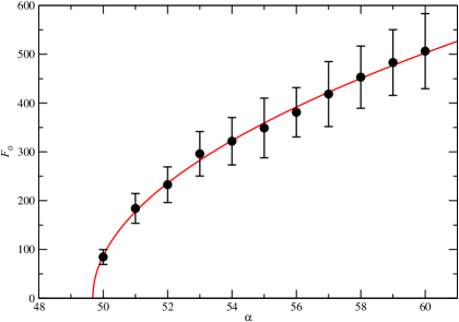
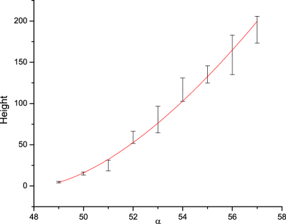
In general, a useful order parameter must be non-zero in one phase, and zero in the rest of the phases. From Figure 2, it is clear that the height of the uniform sub-distribution is a good order parameter for distinguishing between Phase I and Phases II/III. In Figure 3, we show the dependence of on , for kept fixed. From the theory of critical phenomena in statistical physics, we know that statistical fluctuations in a critical system are equally strong at all scales, and thus order parameters are typically scale-free power laws in the vicinity of critical points. Indeed, we find a power law of the form fits the graph in Figure 3 very well, with best-fit values , , and . With such a scaling form, the order parameter is singular at , and the line separating Phase I and II is thus a line of true phase transitions (denoted by a solid curve in Figure 2). In contrast, if we use the peak position of gaussian sub-distribution of above-average stock prices as an ‘order parameter’ to distinguish Phase II from Phase III, we find changing continuously with as we move from Phase II into Phase III. Therefore, as far as we can tell, there is no true phase transitions between Phase II and Phase III, and we use a dashed curve to indicate the crossover from Phase II to Phase III.
Another important result that emerges from the study of critical phenomena is the existence of universality classes of models, each characterized by a set of universal critical exponents. For different values of , we find that the fitted values of are nearly the same. This suggests that is a universal critical exponent. Moreover, these fitted values of are all very close to the universal exponent value of , which is associated with ferromagnetic phase transitions in the mean-field limit (a limit attained by the Ising spin lattice model in infinite dimensions) [26]. This observation is surprising, since traders in our agent-based model do not interact directly with each other, unlike explicit Ising-like interactions between traders in the highly-simplified market models considered by Johansen and co-workers [27, 28].
We believe that through their interactions with the order book, traders experience a retarded Ising-like interaction with other traders. Retarded interactions offer surprises in many other systems. For example, in conventional superconductors, electrostatically repelling electrons experience a retarded, effectively attractive interaction mediated by the ionic lattice, and thereon condensed into Cooper pairs. To test this hypothesis, we define a spin variable for trader , such that
| (3) |
In our toy market model, every agent will buy once and sell once every time step. Therefore, we cannot detect any ferromagnetic or antiferromagnetic transition by plotting as a function of the parameter .
Instead, let us plot the spin-spin correlation as a function of . To define this spin-spin correlation properly, let us start with the definition
| (4) |
We then compute the product
| (5) |
and its time average
| (6) |
If this time average is zero, then and are not correlated.
However, since traders and can only buy and sell one stock each time step, cannot be large. To get a better signal-to-noise ratio, we define the ensemble average
| (7) |
This quantity is large only if traders and are always buying and selling the same stocks. Finally, we define the susceptibility
| (8) |
which will be large only if there are strong trading-induced correlations within the toy financial market.
In each time step , the traders buy one stock each in random order, and after all traders have bought a stock each, they then sell one stock each in a different random order. Therefore, in computing , we add one to for every pair of traders buying the same stock during the buy half-cycle. We then subtract one from for every pair , if had in the sell half-cycle sold the stock that bought in the buy half-cycle, before adding one to for every pair of traders selling the same stock during the sell half-cycle. Before this is repeated for the next time step , we compare the buy half-cycle for and the sell half-cycle for , and subtract one from every pair , if had bought the stock that sold. Finally, we divide this accumulated result by and . For one particular sequence of simulations, with , we find the results shown in Figure 4.
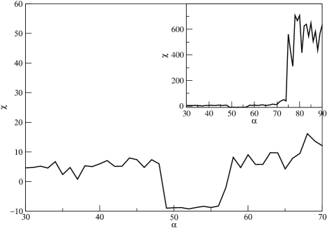
As we can see from Figure 4, is non-zero even for far away from . We suspect this is due to the fact that agents are trading shares, and therefore there will always be a positive statistical background of traders buying or selling the same stocks. There is also a negative statistical background of pairs of traders, one buying a stock, and the other selling the same stock. However, the positive background comes about through the choice of a pair from items, but the negative background comes about through the choice of a pair from items, thus the positive background prevails. This means that the strong dip in around must be due to strong antiferromagnetic correlations mediated by the order book. Interestingly, we also see in a very pronounced signature of the crossover from Phase II to Phase III, which occurs at for .
4 Stochastic Sell and Buy Models
In real markets, traders do not always behave rationally. To introduce some stochasticity into the trading, we can have a fraction of the traders ignore the utility functions, and always trade randomly. Alternatively, we can have all traders trading randomly a fraction of the time. We implement the latter in our simulations, because there is no need to track the stochastic traders individually. If we keep the buy decision deterministic, and make each trader sell a random stock in his or her portfolio a fraction of the time, we end up with a stochastic sell model. Conversely, if we keep the sell decision deterministic, and make each trader buy a random stock from the order book a fraction of the time, we end up with a stochastic buy model. Both are slightly more realistic refinements of the deterministic model. It is also possible to introduce stochasticity into both the buy and sell decisions. This is a more complex model that we intend to study only after we understand the phase diagrams of the deterministic model, and the two simpler stochastic models.
4.1 Stochastic Sell Model
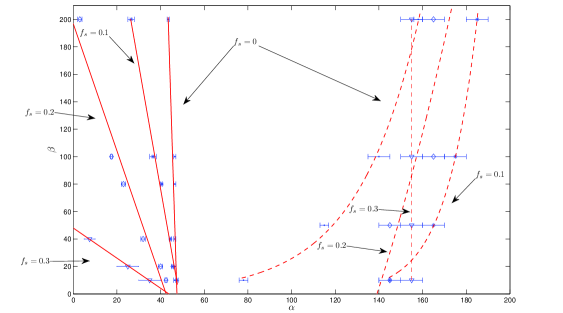
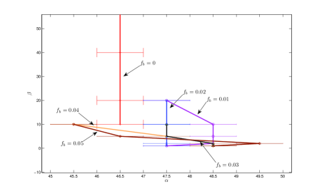
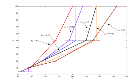
Having developed a good understanding of the deterministic model (), we move on to study the phase diagram of the stochastic sell model, for , , and . In Phases I, II, and III, the typical steady-state price distributions are very similar to those seen in the deterministic model. Also, the order parameters identified for the deterministic model remained good order parameters for the stochastic sell model. After scanning over a broad region in the parameter space, we did not find any new emergent phases, and thus focussed on how the boundaries of the existing phases change as is varied, as shown in Figure 5. We find that, as is increased, Phase II (boom market) expands into the region occupied by Phase I (dead market). A simple extrapolation from the graph of the slope of the phase transition line as a function of suggests that the dead market phase will completely disappear by . This is reassuring, because the dead market phase is not realistic, and we can be confident it will not appear in real markets that are sufficiently noisy. We also checked the character of the I-II phase transition for and , as shown in Figure 6, and find it becoming less abrupt with increasing , until it also becomes a line of crossovers for .
We also find in Figure 5 an interesting behaviour of the line of crossovers: Phase II (boom market) expands at first into Phase III (jammed market) when we go from to , but retreated as we go from to . This suggests that there is an optimum level of trading stochasticity on the sell side, that can drive a boom of the gaussian sub-distribution of above-average stock prices, before this sub-distribution gets stuck in Phase III.
4.2 Stochastic Buy Model
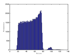
When we go to the stochastic buy model with , the steady-state price distributions are so different from those of the three phases in the deterministic model (see Figure 7) that we cannot recognize the order parameters previously identified. However, when the stochastic buy fraction was lowered to , we find steady-price distributions that closely resemble those of the deterministic model. This means that we can again use the height of the uniform sub-distribution of below-average prices and the peak position of the gaussian sub-distribution of above-average prices as order parameters to characterize the phase diagram of the weakly stochastic buy model.
More importantly, we observe that the sub-distribution of below-average prices is not uniform all the way down to , but develops a shoulder at . When we compare this sub-distribution for , , and , as shown in Figure 8, we see the shoulder price value increases as is increased. This explains why we do not find the uniform sub-distribution for and higher.
As we can see from Figure 9, the effects of introducing stochasticity into the buy side of the deterministic model appears to be the same as when it is introduced into the sell side. The boom market phase expands into the dead and jammed market phases. However, random buy decisions affect the market more strongly than random sell decisions, in the sense that a smaller fraction of random buys produces the same effect on the phase diagram that a larger fraction of random sells would. There is thus strong buy-sell asymmetry at the macroscopic level for this model, which we would not have guessed from the microscopic rules at the agent level.
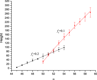
Finally, we look at how the quantitative character of the I-to-II phase transition change when we go from the deterministic model to the stochastic buy model. In Figure 10, we show as a function of for , fitted to a power law of the form . Doing the same for and , we find the exponent going from at , to at , to . Compared to the stochastic sell model, changes very rapidly with , with the I-II transition becoming a crossover by .
5 Summary and Discussions
In conclusion, we described in this paper a bottom-up framework for understanding the hierarchy of complexities that emerge at different levels of realism in agent-based modeling and simulation, and illustrated the approach using a computational study on a simple, deterministic model and its stochastic extensions. In particular, we worked out the phase diagram of the deterministic model, and identified order parameters that can be used to distinguish the three phases: (i) dead market; (ii) boom market; and (iii) jammed market. We find that, as the level of stochasticity is increased, the region occupied by the dead market phase on the phase diagram becomes smaller, and eventually disappears when the market is sufficiently noisy. The transition between the dead market phase and the boom market phase was also found to be in the Ising universality class, with critical exponent in the deterministic model. We provide evidence from the trading history in the simulations that a retarded antiferromagnetic interaction between traders, mediated by the order book, is responsible for this critical behaviour. When we go from the deterministic model to the stochastic buy and sell models, this phase transition becomes a crossover when the market becomes sufficiently noisy.
In our deterministic and stochastic sell model simulations, market rallies or crashes were not observed. In the context of our agent-based models, market rallies are cooperative movements of agent trading strategies from one point within Phase II, to another point within Phase II, where . This movement across the phase diagram can occur under exogeneous forcing, or it can occur endogeneously through positive feedback: if an agent learns that a fundamentalist trading strategy (governed by the price term ) is making him or her more and more money, he or she will make his or her trading strategy even more fundamentalist by increasing ). Similarly, in the context of our agent-based models, the closest analogy to market crashes are cooperative movements of agent trading strategies across the I-II phase transition line. Again, this movement can have an exogeneous origin, or it can occur endogeneously through feedback and learning. In this study, we looked only at steady-state behaviours and worked out the static phase diagrams of three simple models. Ultimately, to study market rallies and crashes, as well as temporally localized features exhibited by more sophisticated models, we need to look more closely at the dynamics of price, volume, and capital distributions.
In the next stage of our programme to understanding agent-based simulations, we will simulate a more realistic model of the financial market, work out its phase diagram, and then couple the agents to an artificial stock index (and hence more strongly to each other), by having their trading strategies be influenced by the stock index. Our immediate goal for doing this would be to check for new emergent phases, and whether it is possible to have market rallies and market crashes without any form of learning in the agents. The long-term goal is to incorporate heterogenuity, memory, and learning into our agent-based models, and map out their diagrams of static and dynamical phases. By extracting the order parameters of these phases, and determining which universality classes they belong to, we then hope to decide which market phases are robust (appearing in a large variety of models with the same gross structures), and which market phases are fragile (appearing only rarely within certain models with very finely tuned parameters). In this way, we aim to develop a picture of the hierarchy of macroscopic phases that emerge at various levels of realism in the agent-based models. Ultimately, we would like to eventually be able to say which market behaviours are robust (does not depend on details of the models, and therefore should appear generically even in markets with very different structures), and which behaviours are fragile (depends sensitively on certain model details, and therefore appear rarely in real-world markets).
Acknowledgments
This work is supported by startup grant SUG 19/07 from the Nanyang Technological University.
References
- [1] R. G. Palmer, W. B. Arthur, J. H. Holland, B. LeBaron, and P. Tayler, “Artificial Economic Life: A Simple Model of a Stockmarket”, Physica D, vol. 75, pp. 264–274, 1994.
- [2] J. M. Epstein, “Agent-Based Computational Models and Generative Social Science”, Complexity, vol. 4, no. 5, pp. 41–60, 1999.
- [3] M. Marsili, “Toy Models and Stylized Realities”, The European Physical Journal B, vol. 55, pp. 169–173, 2007.
- [4] J. D. Farmer, “Market Force, Ecology and Evolution”, Industrial and Corporate Change, vol. 11, no. 5, pp. 895–953, 2002.
- [5] B. LeBaron, “Agent-Based Computational Finance: Suggested Readings and Early Research”, Journal of Economic Dynamics & Control, vol. 24, pp. 679–702, 2000.
- [6] B. LeBaron, “A Builder’s Guide to Agent-Based Financial Markets”, Quantitative Finance, vol. 1, pp. 254–261, 2001.
- [7] L. Tesfatsion, “Agent-Based Computational Economics: Growing Economies From Botton Up”, Artificial Life, vol. 8, no. 1, pp. 55–82, 2002.
- [8] Handbook of Computational Economics, Volume 2: Agent-Based Computational Economics, edited by L. Tesfatsion and K. Judd, North-Holland, 2006.
- [9] M. Levy, H. Levy, and S. Solomon, Microscopic Simulation of Financial Markets, Academic Press, 2000.
- [10] R. N. Mantegna and H. E. Stanley, An Introduction to Econophysics: Correlations and Complexity in Finance, Cambridge University Press, 2008.
- [11] T. Lux and M. Marchesi, “Scaling and Criticality in a Stochastic Multi-Agent Model of a Financial Market”, Nature, vol. 397, no. 6719, pp. 498–500, 1999.
- [12] T. Lux and M. Marchesi, “Volatility Clustering in Financial Markets: A Microsimulation of Interacting Agents”, International Journal of Theoretical and Applied Finance, vol. 3, no. 4, pp. 675–702, 2000.
- [13] M. Raberto, S. Cincotti, S. M. Focardi, and M. Marchesi, “Agent-Based Simulation of a Financial Market”, Physica A, vol. 299, pp. 319–327, 2001.
- [14] B. LeBaron, W. B. Arthur, and R. Palmer, “Time Series Properties of An Artificial Stock Market”, Journal of Economic Dynamics & Control, vol. 23, pp. 1487–1516, 1999.
- [15] P. Bak, M. Paczuski, and M. Shubik, “Price Variations in a Stock Market with Many Agents”, Physica A, vol. 246, pp. 430–453, 1997.
- [16] G. Caldarelli, M. Marsili, and Y.-C. Zhang, “A Prototype Model of Stock Exchange”, Europhysics Letters, vol. 40, no. 5, pp. 479–484, 1997.
- [17] A.-H. Sato and H. Takayasu, “Dynamic Numerical Models of Stock Market Price: From Microscopic Determinism to Macroscopic Randomness”, Physica A, vol. 250, pp. 231–252, 1998.
- [18] D. Chowdhury and D. Stauffer, “A Generalized Spin Model of Financial Markets”, The European Physical Journal B, vol. 8, pp. 477–482, 1999.
- [19] R. Cont and J.-P. Bouchaud, “Herd Behavior and Aggregate Fluctuations in Financial Markets”, Macroeconomic Dynamics, vol. 4, pp. 170–196, 2000.
- [20] S. Maslov, “Simple Model of a Limit Order-Driven Market”, Physica A, vol. 278, pp. 571–578, 2000.
- [21] G. Iori, “A Microsimulation of Traders Activity in the Stock Market: The Role of Heterogenuity, Agents’ Interactions and Trade Frictions”, Journal of Economic Behavior & Organization, vol. 49, pp. 269–285, 2002.
- [22] I. Giardina and J.-P. Bouchaud, “Bubbles, Crashes and Intermittency in Agent Based Market Models”, The European Physical Journal B, vol. 31, pp. 421–437, 2003.
- [23] I. Giardina and J.-P. Bouchaud, “Volatility Clustering in Agent Based Market Models”, Physica A, vol. 324, pp. 6–16, 2003.
- [24] C. F. Moukarzel, S. Gonçalves, J. R. Iglesias, M. Rodríguez-Achach, and R. Huerta-Quintanilla, “Wealth Condensation in a Multiplicative Random Asset Exchange Model”, The European Physical Journal: Special Topics, vol. 143, pp. 75–79, 2007.
- [25] L. Gauvin, J. Vannimenus, and J.-P. Nadal, “Phase Diagram of a Schelling Segregation Model”, The European Physical Journal B, vol. 70, pp. 293–304, 2009.
- [26] J. J. Binney, N. J. Dowrick, A. J. Fisher, and M. E. J. Newman, The Theory of Critical Phenomena: An Introduction to the Renormalization Group, Oxford University Press, 1992.
- [27] A. Johansen and D. Sornette, “Modeling the Stock Market Prior to Large Crashes”, The European Physical Journal B, vol. 9, no. 1, pp. 167–174, 1999.
- [28] A. Johansen, O. Ledoit, and D. Sornette, “Crashes As Critical Points”, International Journal of Theoretical and Applied Finance, vol. 3, no. 2, pp. 219–255, 2000.