Model-Independent Signatures of New Physics in non-Gaussianity

Abstract

We compute the model-independent contributions to the primordial bispectrum and trispectrum in de Sitter space due to high-energy physics. We do this by coupling a light inflaton to an auxiliary heavy field, and then evaluating correlation functions in the Schwinger-Keldysh “in-in” formalism. The high-energy physics produces corrections parametrized by $H/M$ where $H$ is the scale of inflation and $M$ is the mass of the heavy field. The bispectrum peaks near the elongated shape, but otherwise contains no features. The trispectrum receives no corrections at order $H/M$.

I Introduction

The leading paradigm for understanding the first moments of the Universe is known as Inflationary Theory, wherein space rapidly expanded in a very brief period of time Guth:1980zm ; Linde:1981mu ; Albrecht:1982wi ; Linde:1983gd . An important property of inflation is that its low-energy observables are sensitive to high-energy physics Brandenberger:1999sw ; Greene:2005aj . This non-decoupling of energy scales, while sometimes confounding, can also be used as a probe of ultra high-energy physics such as the effects of quantum gravity. In order to verify, constrain or eliminate classes of such theories, one must understand the precise relationship between low- and high-energy physics in inflationary theory.

The primary low-energy inflationary observables are the correlation functions of primordial perturbations of the quantum field responsible for the inflation. Since such perturbations seed the observed temperature fluctuations in the cosmic microwave background (CMB), one could use the CMB to gain insight into high-energy physics. This is particularly exciting given the recent explosion in precision data by WMAP wmap7 , Planck planck , Euclid euclid and possibly CMBPol/Inflation Probe cmbpol .

The inflationary fluctuation spectrum has been observed to be nearly Gaussian wmap7 , and the two-point correlation probes the free theory:

$$\langle\varphi_{\bf k}\varphi_{\bf p}\rangle\sim P_{\varphi}(k)(2\pi)^{3}\delta^{3}({\bf k}+{\bf p}),$$

Higher-point correlations then probe the interactions by measuring the non-Gaussianity of the statistics. The three-point correlation is commonly referred to as the bispectrum and is simply the 3-field analog of the power spectrum:

$$\langle\varphi_{{\bf k}_{1}}\varphi_{{\bf k}_{2}}\varphi_{{\bf k}_{3}}\rangle\sim B_{\varphi}({\bf k}_{1},{\bf k}_{2},{\bf k}_{3})(2\pi)^{3}\delta^{3}\left({\bf k}_{1}+{\bf k}_{2}+{\bf k}_{3}\right).$$ (1)

This diagnostic has quickly become an essential tool in constraining inflation models Komatsu:2009kd . While as yet there have only been hints of non-Gaussianity Yadav:2007yy ; Senatore:2009gt , a definitive measurement will occur soon from Planck planck . At the most elementary level, non-Gaussianity can be categorized according to the shape of the triangle formed by the fields’ momentum vectors at which the amplitude $B_{\varphi}$ is maximized. The ‘squeezed’ shape, $k_{1}\sim k_{2}$ and $k_{3}\sim 0$, dominates for local interactions such as $\varphi(x)^{3}$ Komatsu:2001rj , and occur well outside the horizon. The ‘equilateral’ shape $k_{1}\sim k_{2}\sim k_{3}$ occur primarily at the time of horizon-crossing and dominates for higher-derivative interactions such as found in the Dirac-Born-Infeld theory Creminelli:2003iq ; Alishahiha:2004eh . The ‘elongated’ shape, where $k_{1}+k_{2}\sim k_{3}$, dominates for an initial vacuum state modified away from Bunch-Davies, and often enhances the other types as well Holman:2007na ; Meerburg:2009ys ; Meerburg:2009fi ; Chen:2010bka ; Ganc:2011dy ; Chialva:2011hc . A nice heuristic way of understanding this relationship is that the more squeezed the triangle, the later it originated. In anticipation of the upcoming Planck data, a more sophisticated technique has recently been pioneered by Fergusson, Liguori, and Shellard Fergusson:2010dm . This analysis is model-independent in the sense that it does not assume a particular template shape (squeezed, equilateral, or elongated) and so requires an equally sophisticated model-independent theoretical basis for understanding.

In order to meet this need, the fundamental question how to construct the low-energy effective action in inflationary backgrounds had to be answered. We did so in Jackson:2010cw ; Jackson:2011qg ; Jackson:2012qp . This new method allows one to reliably compute universal corrections to primordial correlation functions. The approach is model-independent in the sense that we begin with the general form of an ultraviolet-complete action and obtain an answer in terms of a small number of free parameters that in principle encodes all the possible unknown physics. The fundamental organizing principle is not yet known. Nevertheless we can simply compute the effects in any specific model and generalize from there. We have previously used this technique to compute the primordial power spectrum, here we will apply it to compute the 3- and 4-point correlations. An important difference with flat space effective field theory is that a heavy field of mass $M$ will correct the correlation function already at order $H/M$, where $H$ is the scale of inflation. Moreover, as will shall show, the leading contribution to the bispectrum is of the elongated shape just as previous studies surmised Holman:2007na ; Meerburg:2009ys ; Meerburg:2009fi ; Ganc:2011dy ; Chialva:2011hc .

This article is structured as follows. In §2 we briefly summarize the technical framework by which high-energy physics can consistently be integrated out of a theory in an inflating background. In §3 we calculate the bispectrum corrections, and in §4 those for the trispectrum. In §5 we conclude and offer some remarks about detectability and future directions.

II Setup

II.1 The Generic Action

We will consider the most general field theory containing a light scalar field fluctuation $\varphi$ renormalizably coupled to a heavy field $\chi$:

$$S_{\rm fl} = \int d^{4}x\sqrt{g}\left[\frac{1}{2}(\partial\varphi)^{2}+\frac{1}{2}(\partial\chi)^{2}+\frac{1}{2}M^{2}\chi^{2}\right.$$ (2)

$$\left.+\frac{g_{0}}{3!}\varphi^{3}+\frac{\lambda_{0}}{4!}\varphi^{4}+\frac{g_{1}}{2}\varphi^{2}\chi+\frac{\lambda_{1}}{3!}\varphi^{3}\chi\right].$$

This is similar to the theory considered in Jackson:2010cw ; Jackson:2011qg , but we have added a $\varphi^{3}\chi$ interaction to generate non-Gaussian interactions, and will now include self-interactions in our result . We will take the metric background to be exact de Sitter space,

$$ds^{2}=-dt^{2}+a(t)^{2}d{\bf x}^{2},$$

where ${\dot{a}}/a\equiv H={\rm constant}$.

II.2 The In-In Formalism and Schwinger-Keldysh Basis

In the Schwinger-Keldysh “in-in” formalism, at some early time $t_{\rm in}$ we begin with a pure state $|{\rm in}(t_{\rm in})\rangle$, then evolve the system for the bra- and ket-state separately until some late time $t$, when we evaluate the expectation value Calzetta:1986cq :

$$\langle\mathcal{O}(t)\rangle \equiv \langle{\rm in}(t)|\mathcal{O}(t)|{\rm in}(t)\rangle$$

$$= \langle{\rm in}(t_{\rm in})|e^{i\int_{t_{\rm in}}^{t}dt^{\prime}H(t^{\prime})}\mathcal{O}(t)e^{-i\int_{t_{\rm in}}^{t}dt^{\prime\prime}H(t^{\prime\prime})}|{\rm in}(t_{\rm in})\rangle.$$

Traditionally, the in-state $|{\rm in}\rangle$ is taken to be the Bunch-Davies vacuum state Bunch:1978yq , but this is not necessarily so. Expanding cosmological backgrounds allow for a more general class of vacua, which can be heuristically considered to be excited states of inflaton fluctuations. In the present context, we will find that integrating out high-energy physics generically results in corrections to the density matrix, which can be interpreted this way.

If we denote the fields representing the “evolving” ket to be $\{\varphi_{+},\chi_{+}\}$ and those for the “devolving” bra to be $\{\varphi_{-},\chi_{-}\}$, the in-in expectation value (II.2) can be computed from the action

$$\mathcal{S}\equiv S[\varphi_{+},\chi_{+}]-S[\varphi_{-},\chi_{-}].$$ (4)

together with the constraint that $\varphi_{+}(t)=\varphi_{-}(t)$. It is then helpful to transform into the Keldysh basis,

$$\ {\bar{\varphi}} \equiv (\varphi_{+}+\varphi_{-})/2,\hskip 36.135pt{\Phi}\equiv\varphi_{+}-\varphi_{-},$$

$${\bar{\chi}} \equiv (\chi_{+}+\chi_{-})/2,\hskip 36.135pt{\rm X}\equiv\chi_{+}-\chi_{-}.$$

In this basis the action (4) equals

$$\mathcal{S}[{\bar{\varphi}},{\Phi},{\bar{\chi}},{\rm X}]=-\int d^{3}{\bf x}dt\ a(t)^{3}\left[\partial{\bar{\varphi}}\partial\Phi+\partial{\bar{\chi}}\partial{\rm X}+M^{2}{\bar{\chi}}{\rm X}\right.$$

$$\hskip 36.135pt+\frac{g_{0}}{2}\left({\bar{\varphi}}^{2}\Phi+\frac{1}{12}\Phi^{3}\right)+\frac{\lambda_{0}}{3!}\left({\bar{\varphi}}^{3}\Phi+\frac{1}{4}{\bar{\varphi}}\Phi^{3}\right)$$

$$\hskip 36.135pt\left.+g_{1}{\bar{\varphi}}\Phi{\bar{\chi}}+\frac{g_{1}}{2}{\bar{\varphi}}^{2}{\rm X}+\frac{\lambda_{1}}{2}{\bar{\varphi}}^{2}\Phi{\bar{\chi}}+\frac{\lambda_{1}}{3!}{\bar{\varphi}}^{3}{\rm X}\right].$$

Fluctuation solutions are easiest written in the conformal time $\tau$,

$$dt\equiv a(\tau)d\tau.$$

The free field solutions are then

$$U_{\bf k}(\tau) = \frac{H}{\sqrt{2k^{3}}}(1-ik\tau)e^{-ik\tau},$$

$$V_{\bf k}(\tau) \approx \frac{1}{a(\tau)}\frac{\exp\left[-i\int^{\tau}_{\tau_{\rm in}}d\tau^{\prime}\sqrt{k^{2}+\frac{M^{2}}{H^{2}\tau^{\prime 2}}}\right]}{\sqrt{2}\left(k^{2}+\frac{M^{2}}{H^{2}\tau^{2}}\right)^{1/4}}$$

where for the latter we have used the WKB approximation which is always valid for $H/M\ll 1$.

We will also need the Green’s and Wightman functions in the Keldysh basis; see Jackson:2011qg for an explanation of their interpretation. Fourier transforming into comoving momentum, the retarded Green’s function $G^{R}$ can be written in terms of the fluctuation solutions,

$$G^{R}_{\bf k}(\tau_{1},\tau_{2}) \equiv i\langle{\bar{\varphi}}_{\bf k}(\tau_{1})\Phi_{\bf-k}(\tau_{2})\rangle$$

$$= -2\theta(\tau_{1}-\tau_{2}){\rm Im}\left[U_{\bf k}(\tau_{1})U^{*}_{\bf k}(\tau_{2})\right].$$

The advanced Green’s function $G^{A}$ is then simply the time-reversal of this:

$$G^{A}_{\bf k}(\tau_{1},\tau_{2})\equiv G^{R}_{\bf k}(\tau_{2},\tau_{1}).$$

A similar procedure applies for ${\bar{\chi}}$ using its corresponding retarded Green’s function $\mathcal{G}^{R}$,

$$\mathcal{G}^{R}_{\bf k}(\tau_{1},\tau_{2}) \equiv i\langle{\bar{\chi}}_{\bf k}(\tau_{1}){\rm X}_{\bf-k}(\tau_{2})\rangle$$

$$= -2\theta(\tau_{1}-\tau_{2}){\rm Im}\left[V_{\bf k}(\tau_{1})V^{*}_{\bf k}(\tau_{2})\right].$$

The Wightman functions are

$$F_{\bf k}(\tau_{1},\tau_{2}) = \langle{\bar{\varphi}}_{\bf k}(\tau_{1}){\bar{\varphi}}_{\bf-k}(\tau_{2})\rangle$$

$$= {\rm Re}\left[U_{\bf k}(\tau_{1})U^{*}_{\bf k}(\tau_{2})\right],$$

$$0 = \langle\Phi_{\bf k}(\tau_{1})\Phi_{\bf-k}(\tau_{2})\rangle,$$

$$\mathcal{F}_{\bf k}(\tau_{1},\tau_{2}) = \langle{\bar{\chi}}_{\bf k}(\tau_{1}){\bar{\chi}}_{\bf-k}(\tau_{2})\rangle$$

$$= {\rm Re}\left[V_{\bf k}(\tau_{1})V^{*}_{\bf k}(\tau_{2})\right],$$

$$0 = \langle{\rm X}_{\bf k}(\tau_{1}){\rm X}_{\bf-k}(\tau_{2})\rangle.$$

We will now use these to compute higher-point correlation functions in the interacting theory.

III Bispectrum Corrections

III.1 Definitions

A more precise definition of the bispectrum given by eq. (1) is

$$B_{\varphi}({\bf k}_{1},{\bf k}_{2},{\bf k}_{3})(2\pi)^{3}\delta^{3}\left({\bf k}_{1}+{\bf k}_{2}+{\bf k}_{3}\right)\equiv$$ (7)

$$\langle{\rm in}(0)|{\bar{\varphi}}_{{\bf k}_{1}}(0){\bar{\varphi}}_{{\bf k}_{2}}(0){\bar{\varphi}}_{{\bf k}_{3}}(0)|{\rm in}(0)\rangle,$$

where the time evolution of the in-state is given by

$$|{\rm in}(\tau)\rangle=e^{-i\int^{\tau}_{\tau_{\rm in}}dt^{\prime}\mathcal{H}(t^{\prime})}|{\rm in}(\tau_{\rm in})\rangle,$$

recalling that $\tau\rightarrow 0^{-}$ corresponds to future infinity. From henceforth we will assume a Bunch-Davies in-state. There are two types of contributions to $B_{\varphi}$: those arising from self-interactions of the $\varphi$ field, and those mediated by the heavy field $\chi$ coupled to $\varphi$. Since they have qualitatively different behavior, we will consider each separately.

III.2 Self Interactions

Let us first consider the simplest possible interaction: that arising from the $\varphi^{3}$ interaction. In the Schwinger-Keldysh basis this produces two diagrams, shown in Figure 1. These are given by (we henceforth omit the momentum-conserving delta-function and just assume that ${\bf k}_{1}+{\bf k}_{2}+{\bf k}_{3}=0$):

$$B_{\varphi}^{\rm self} = \frac{(-ig_{0})}{(2\pi)^{3}}\int^{0}_{\tau_{\rm in}}d\tau\ a(\tau)^{4}$$

$$\times\left.\Big{(}[-iG^{R}_{{\bf k}_{1}}(0,\tau)]F_{{\bf k}_{2}}(0,\tau)F_{{\bf k}_{3}}(0,\tau)+\ {\rm permutations}\right.$$

$$+\left.\frac{1}{4}[-iG^{R}_{{\bf k}_{1}}(0,\tau)][-iG^{R}_{{\bf k}_{2}}(0,\tau)][-iG^{R}_{{\bf k}_{3}}(0,\tau)]\right).$$

Writing out the Green and Wightman functions in terms of the functions $U_{\bf k}(\tau),U_{\bf k}^{*}(\tau)$, and using the fact that $U_{\bf k}(0)=U_{\bf k}^{*}(0)=H/\sqrt{2k^{3}}$ yields

$$B_{\varphi}^{\rm self}=\frac{ig_{0}}{2(2\pi)^{3}(2k_{1}k_{2}k_{3})^{3/2}H}\int_{\tau_{\rm in}}^{0}\frac{d\tau}{\tau^{4}}\Big{[}{U}_{{\bf k}_{1}}(\tau){U}_{{\bf k}_{2}}(\tau)U_{{\bf k}_{3}}(\tau)$$

$$+{U}^{*}_{{\bf k}_{1}}(\tau){U}_{{\bf k}_{2}}(\tau)U_{{\bf k}_{3}}(\tau)+{\rm permutations}-\ {\rm c.c.}\Big{]}.$$

The integrals will converge in the far past by slightly rotating the path of integration into the complex plane, so that $\tau_{\rm in}\rightarrow-\infty(1+i\epsilon)$. For the far future, we choose a cutoff at $\mu\rightarrow 0^{-}$, so that the most singular part of the resultant integrals are:

$$\int^{\mu}_{-\infty(1+i\epsilon)}\frac{d\tau}{\tau^{n}}e^{-ik\tau}\sim-\frac{\mu^{1-n}}{n-1}+\mathcal{O}\left((k\mu)^{-n}\right).$$ (8)

Thus the late-time correlation is approximately

$$B_{\varphi}^{\rm self}\approx\frac{g_{0}\mu^{-3}H^{2}}{6(2\pi k_{1}k_{2}k_{3})^{3}}.$$

This correlation peaks when $k_{i}\approx 0$, corresponding to the squeezed shapes of the momentum triangle. Note that this is not quite the same local interaction studied by Komatsu and Spergel Komatsu:2001rj , which introduce nonlinearities into the late-time gauge-independent parameter $\zeta$, whereas we deal with the field fluctuation $\varphi$ and integrate the interactions from the far past. Defining the non-linearity parameter $f^{\rm self}_{\rm NL}\sim B^{\rm self}_{\varphi}/P^{2}_{\varphi}\sim k^{-3}$, the self interaction is seen to have a strong red scaling. This may possibly be measurable in the near future Sefusatti:2009xu using the leverage provided by combining the Planck planck and Euclid euclid datasets. Employing two self interactions will produce loop corrections of order $B^{\rm self}_{\varphi}~{}\sim~{}g_{0}\lambda_{0}H^{2}$ and $B^{\rm self}_{\varphi}~{}\sim~{}g_{0}^{3}$ as shown in Figure 2, but slow-roll assumes that the these couplings are small and so these contributions are subleading.

Figure 1: Lowest-order contributions to primordial bispectrum induced by the self-interaction of the light field. Single solid lines indicate contractions of ${\bar{\varphi}}$, dashed single lines indicate those of $\Phi$.

Figure 2: Higher-order bispectrum contribution induced by multiple self-interactions of the light field. These can be neglected in slow-roll inflation due to the strong constraints on the couplings.

III.3 High-Energy Correction A

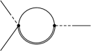
A

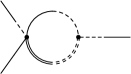
B

C

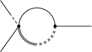
D

Figure 3: Contributions to primordial non-Gaussianity induced by the heavy field. The double lines indicate the heavy field components $\{{\bar{\chi}},{\rm X}\}$, with notation analogous to Figure 1.

We now turn to the corrections generated by high-energy physics. To leading order in the heavy field, there are four such corrections, shown diagramatically in Figure 3. Since $\tau_{2}\leq\tau_{1}$ we need only consider corrections containing $G^{R}(\tau_{1},\tau_{2})$ (as opposed to corrections containing $G^{A}(\tau_{1},\tau_{2})$).

The first correction is given by

$$B_{\varphi}^{A} = \frac{(-ig_{1})(-i\lambda_{1})}{(2\pi)^{3}}\int^{0}_{\tau_{\rm in}}d\tau_{1}\ a(\tau_{1})^{4}\int^{0}_{\tau_{\rm in}}d\tau_{2}\ a(\tau_{2})^{4}\times$$

$$\int\frac{d^{3}{\bf q}}{(2\pi)^{3}}\Big{(}[-iG^{R}_{{\bf k}_{1}}(0,\tau_{1})]F_{{\bf k}_{2}}(0,\tau_{1})F_{{\bf q}}(\tau_{1},\tau_{2})\times$$

$$\mathcal{F}_{{\bf q}-{\bf k}_{3}}(\tau_{1},\tau_{2})[-iG^{A}_{{\bf k}_{3}}(\tau_{2},0)]+\ {\rm permutations}\Big{)}.$$

Writing out the Green and Wightman functions in terms of $U$’s and $V$’s, we see there are now several types of vertices, depending on the permutation of conjugation. The first is

$$\mathcal{A}_{1}({\bf k}_{1},{\bf k}_{2}) \equiv \int_{\tau_{\rm in}}^{0}d\tau\ a(\tau)^{4}{U}_{{\bf k}_{1}}(\tau){U}_{{\bf k}_{2}}(\tau)V^{*}_{-({\bf k}_{1}+{\bf k}_{2})}(\tau)f(\tau)$$

$$=-\frac{1}{2\sqrt{2k_{1}^{3}k_{2}^{3}}H}\int_{\tau_{\rm in}}^{0}\frac{d\tau}{\tau^{3}}\frac{\left(1-ik_{1}\tau\right)\left(1-ik_{2}\tau\right)}{\left(|{{\bf k}_{1}+{\bf k}_{2}}|^{2}+\frac{M^{2}}{H^{2}\tau^{2}}\right)^{1/4}}f(\tau)$$

$$\times\exp\left[-i(k_{1}+k_{2})\tau+i\int^{\tau}_{\tau_{\rm in}}d\tau^{\prime}\sqrt{|{{\bf k}_{1}+{\bf k}_{2}}|^{2}+\frac{M^{2}}{H^{2}\tau^{\prime 2}}}\right],$$

where we have introduced a function $f(\tau)$ to account for any step-functions. As first noted in Jackson:2010cw , by rescaling $u\equiv H\tau/M$ the vertex $\mathcal{A}_{1}({\bf k}_{1},{\bf k}_{2})$ admits a stationary phase approximation at the energy-conservation moment

$$k_{1}+k_{2}=\sqrt{|{\bf k}_{1}+{\bf k}_{2}|^{2}+u_{c}^{-2}}.$$ (9)

The solution to this defines the New Physics Hypersurface (NPH),

$$u_{c}^{-1}=-\sqrt{2k_{1}k_{2}(1-\cos\theta)},\hskip 21.68121pt\cos\theta=\frac{{\bf k}_{1}\cdot{\bf k}_{2}}{k_{1}k_{2}}.$$

Then to leading order in $H/M$ the amplitude is

$$\mathcal{A}_{1}({\bf k}_{1},{\bf k}_{2}) \approx -\frac{\sqrt{\pi i}f(\tau_{c})e^{-i\frac{M}{H}\sqrt{|{\bf k}_{1}+{\bf k}_{2}|^{2}u_{\rm in}^{2}+1}}}{2\sqrt{k_{1}k_{2}}\left[2k_{1}k_{2}(1-\cos\theta)\right]^{1/4}\sqrt{HM}}$$ (10)

$$\times\left(\frac{{k_{1}+k_{2}+\sqrt{2k_{1}k_{2}(1-\cos\theta)}}}{\sqrt{|{{\bf k}_{1}+{\bf k}_{2}}|^{2}+u_{\rm in}^{-2}}+|u_{\rm in}|^{-1}}\right)^{-i\frac{M}{H}}.$$

The physics of this is clear. This diagram accounts for the threshold production/decay of heavy particles at high redshift in the early universe. Note that in order to evaluate $f(\tau_{c})$, one should use the step-function appropriately “averaged” due to the Gaussian fluctuations:

$$\theta(\tau)=\left\{\begin{array}[]{cc}1&{\rm if}\ \tau>0,\\ \nicefrac{{1}}{{2}}&{\rm if}\ \tau=0,\\ 0&{\rm if}\ \tau<0.\\ \end{array}\right.$$ (11)

The second possible vertex is identical to $\mathcal{A}_{1}$ but with one $U$ conjugated. This has only imaginary-time saddlepoint solutions. Since our $\tau$-integral is confined to the real axis we will never pass over this point in our integration, and so this amplitude will be suppressed as $\mathcal{A}_{2}\sim{\rm erf}(\frac{M}{H})\sim\frac{H}{M}e^{-(M/H)^{2}}$, allowing us to neglect such interactions. Finally we consider $\mathcal{A}_{3}$ which has both $U$’s conjugated and so admits no saddlepoint solutions, and thus can also be neglected. Note also that while there are actually two solutions (differing in sign), we limit ourselves to the solution for which $u_{c}<0$, corresponding to the inflating phase (see Jackson:2011qg for details on this).

We can now perform a similar analysis of four-field interactions. The first such vertex is

$$\mathcal{B}_{1}({\bf k}_{1},{\bf k}_{2},{\bf k}_{3})$$

$$\equiv \int_{\tau_{\rm in}}^{0}d\tau\ a(\tau)^{4}{U}_{{\bf k}_{1}}(\tau){U}_{{\bf k}_{2}}(\tau){U}_{{\bf k}_{3}}(\tau)V^{*}_{-({\bf k}_{1}+{\bf k}_{2}+{\bf k}_{3})}(\tau)f(\tau)$$

$$= -\frac{1}{4\sqrt{k_{1}^{3}k_{2}^{3}k_{3}^{3}}}\int^{0}_{\tau_{\rm in}}\frac{d\tau}{\tau^{3}}\frac{\left(1-ik_{1}\tau\right)\left(1-ik_{2}\tau\right)\left(1-ik_{3}\tau\right)}{\left(|{\bf k}_{1}+{\bf k}_{2}+{\bf k}_{3}|^{2}+\frac{M^{2}}{H^{2}\tau^{2}}\right)^{1/4}}$$

$$\times\exp\left[-i(k_{1}+k_{2}+k_{3})\tau+i\int_{\tau_{\rm in}}^{\tau}d\tau^{\prime}\sqrt{|{\bf k}_{1}+{\bf k}_{2}+{\bf k}_{3}|^{2}+\frac{M^{2}}{H^{2}\tau^{\prime 2}}}\right].$$

Using the same rescaling, the stationary phase is now at

$$u_{c}^{-1}=-\sqrt{(k_{1}+k_{2}+k_{3})^{2}-|{\bf k}_{1}+{\bf k}_{2}+{\bf k}_{3}|^{2}}$$

which always exists (that is, it is real). To leading order, the amplitude is

$$\mathcal{B}_{1}({\bf k}_{1},{\bf k}_{2},{\bf k}_{3}) \approx \frac{i\sqrt{\pi iM}f(\tau_{c})e^{-i\frac{M}{H}\sqrt{|{\bf k}_{1}+{\bf k}_{2}+{\bf k}_{3}|^{2}u_{\rm in}^{2}+1}}}{4\sqrt{Hk_{1}k_{2}k_{3}}}$$

$$\times \left[(k_{1}+k_{2}+k_{3})^{2}-|{\bf k}_{1}+{\bf k}_{2}+{\bf k}_{3}|^{2}\right]^{-3/4}$$

$$\times\left(\frac{{k_{1}+k_{2}+k_{3}+\sqrt{(k_{1}+k_{2}+k_{3})^{2}-|{\bf k}_{1}+{\bf k}_{2}+{\bf k}_{3}|^{2}}}}{\sqrt{|{{\bf k}_{1}+{\bf k}_{2}}+{\bf k}_{3}|^{2}+u_{\rm in}^{-2}}+|u_{\rm in}|^{-1}}\right)^{-i\frac{M}{H}}.$$

A similar vertex, but with the third light field outgoing (we place a bar there to remind us of this), is:

$$\mathcal{B}_{2}({\bf k}_{1},{\bf k}_{2}|{\bf k}_{3})$$

$$\equiv \int_{\tau_{\rm in}}^{0}d\tau\ a(\tau)^{4}{U}_{{\bf k}_{1}}(\tau){U}_{{\bf k}_{2}}(\tau){U}^{*}_{{\bf k}_{3}}(\tau)V^{*}_{-({\bf k}_{1}+{\bf k}_{2}+{\bf k}_{3})}(\tau)f(\tau)$$

$$= -\frac{1}{4\sqrt{k_{1}^{3}k_{2}^{3}k_{3}^{3}}}\int^{0}_{\tau_{\rm in}}\frac{d\tau}{\tau^{3}}\frac{\left(1-ik_{1}\tau\right)\left(1-ik_{2}\tau\right)\left(1+ik_{3}\tau\right)}{\left(|{\bf k}_{1}+{\bf k}_{2}+{\bf k}_{3}|^{2}+\frac{M^{2}}{H^{2}\tau^{2}}\right)^{1/4}}$$

$$\times\exp\left[-i(k_{1}+k_{2}-k_{3})\tau+i\int_{\tau_{\rm in}}^{\tau}d\tau^{\prime}\sqrt{|{\bf k}_{1}+{\bf k}_{2}+{\bf k}_{3}|^{2}+\frac{M^{2}}{H^{2}\tau^{\prime 2}}}\right].$$

The stationary phase for this is at

$$u_{c}^{-1}=-\sqrt{(k_{1}+k_{2}-k_{3})^{2}-|{\bf k}_{1}+{\bf k}_{2}+{\bf k}_{3}|^{2}}.$$

This is not always real, and one must take care. To leading order, the amplitude is

$$\mathcal{B}_{2}({\bf k}_{1},{\bf k}_{2}|{\bf k}_{3}) \approx \frac{i\sqrt{\pi iM}f(\tau_{c})e^{-i\frac{M}{H}\sqrt{|{\bf k}_{1}+{\bf k}_{2}+{\bf k}_{3}|^{2}u_{\rm in}^{2}+1}}}{4\sqrt{Hk_{1}k_{2}k_{3}}}$$

$$\times \left[(k_{1}+k_{2}-k_{3})^{2}-|{\bf k}_{1}+{\bf k}_{2}+{\bf k}_{3}|^{2}\right]^{-3/4}$$

$$\times\left(\frac{{k_{1}+k_{2}-k_{3}+\sqrt{(k_{1}+k_{2}-k_{3})^{2}-|{\bf k}_{1}+{\bf k}_{2}+{\bf k}_{3}|^{2}}}}{\sqrt{|{{\bf k}_{1}+{\bf k}_{2}}+{\bf k}_{3}|^{2}+u_{\rm in}^{-2}}+|u_{\rm in}|^{-1}}\right)^{-i\frac{M}{H}}.$$

Based on this, it is easy to see that the amplitude is

$$B^{A}_{\varphi}=\frac{g_{1}\lambda_{1}}{8(2\pi)^{3}}\frac{H^{3}}{(2k_{1}k_{2}k_{3})^{3/2}}\int\frac{d^{3}{\bf q}}{(2\pi)^{3}}$$

$$\Big{[}\mathcal{A}_{1}({\bf q},-{\bf k}_{3})\mathcal{B}_{1}^{*}({\bf k}_{2},{\bf q},{\bf k}_{1})+{\rm c.c.}$$

$$-\mathcal{A}_{1}({\bf q},-{\bf k}_{3})\mathcal{B}_{2}^{*}({\bf k}_{2},{\bf q}|{\bf k}_{1})+\mathcal{A}_{1}({\bf q},-{\bf k}_{3})\mathcal{B}_{2}^{*}({\bf k}_{1},{\bf q}|{\bf k}_{2})+{\rm c.c.}$$

$$\hskip 144.54pt+\ {\rm permutations}\Big{]}.$$

But the $k_{1}\leftrightarrow k_{2}$ symmetry will cancel the $\mathcal{B}_{2}$-dependent terms, leaving only the $\mathcal{B}_{1}$-dependent terms.

Examining the loop integral in the expression above, the integrand contains a rapidly oscillating component due to the difference in vertex interaction times is

$$\left(\frac{|{\bf k}_{1}+{\bf k}_{2}|+q+\sqrt{(|{\bf k}_{1}+{\bf k}_{2}|+q)^{2}-|{\bf k}_{1}+{\bf k}_{2}+{\bf q}|^{2}}}{{k_{1}+k_{2}+q+\sqrt{(k_{1}+k_{2}+q)^{2}-|{\bf k}_{1}+{\bf k}_{2}+{\bf q}|^{2}}}}\right)^{-i\frac{M}{H}}.$$ (12)

Given such rapid oscillations of this phase, this could potentially be evaluated using (another) stationary phase approximation. However, one can easily convince themself that there exist no such stationary phase points except in the trivial case of $k_{3}=|{\bf k}_{1}+{\bf k}_{2}|=k_{1}+k_{2}$, meaning the phase is identically zero. Thus, for all configurations except this, the amplitude is suppressed as $H/M$.

To evaluate the integral, we then expand near this point,

$$\kappa_{12} \equiv k_{1}+k_{2}-k_{3},$$

and the oscillating component (12) simplifies to

$$e^{i\frac{M}{H}\kappa_{12}/\sqrt{2qk_{3}(1-\cos\theta)}},$$

where $\theta$ is the angle between $-{\bf k}_{3}={\bf k}_{1}+{\bf k}_{2}$ and ${\bf q}$.

Now we must do the integral over ${\bf q}$. As done in earlier work Jackson:2010cw ; Jackson:2011qg , we first use the azimuthal symmetry around ${\bf k}_{3}$ to simplify the 3d integral into just two variables,

$$\int\frac{d^{3}{\bf q}}{(2\pi)^{3}}\rightarrow\frac{1}{(2\pi)^{2}}\int q^{2}dqd(1-\cos\theta).$$

We wish to transform this into the $(u,E)$-basis given by

$$u^{-1} \equiv -\sqrt{2k_{3}q(1-\cos\theta)},$$ (13)

$$E\equiv Mq|u| = M\sqrt{\frac{q}{2k_{3}(1-\cos\theta)}}.$$

These can be easily inverted as

$$q=\frac{E}{M|u|},\hskip 28.90755pt1-\cos\theta=\frac{M}{2k_{3}E|u|},$$

so that the ${\bf q}$-integral then transforms as

$$\int\frac{d^{3}\bf q}{(2\pi)^{3}}\rightarrow-\frac{1}{(2\pi)^{2}M^{2}k_{3}}\int\frac{duEdE}{u^{5}}.$$ (14)

The integrand transforms as

$$\mathcal{A}_{1}({\bf q},-{\bf k}_{3})\mathcal{B}_{1}^{*}({\bf k}_{2},{\bf q},{\bf k}_{1})\rightarrow\frac{\pi|u|^{3}Me^{-i\frac{M}{H}\kappa_{12}u}}{8HE\sqrt{k_{1}k_{2}k_{3}}}+\mathcal{O}(\kappa_{12}).$$ (15)

Noting that $E$ is a physical rather than a comoving scale, we can now easily place limits on the region of integration in terms of the physical cutoff $\Lambda$. Recalling that at the moment of interaction the energies of the light fields will sum to the energy of the heavy field, and so it is this latter quantity that we must place the bound of $\Lambda$ on. The minimal energy bound comes from the geometrical constraint $\cos\theta\geq-1$. The bounds on the loop energy are then:

$$\frac{M}{4k_{3}|u|}\leq E \leq\Lambda-k_{3}|u|M,$$

$$-\frac{\Lambda+\sqrt{\Lambda^{2}-M^{2}}}{2Mk_{3}}\leq u \leq-\frac{\Lambda-\sqrt{\Lambda^{2}-M^{2}}}{2Mk_{3}}.$$

The measure (14) and integrand (15) combine to produce an $E$-integral which is trivial,

$$\int^{\Lambda-k_{3}|u|M}_{\frac{M}{4k_{3}|u|}}dE=\Lambda-k_{3}|u|M-\frac{M}{4k_{3}|u|}.$$

Now including the factor of $u^{-2}$ from the measure and vertex evaluations (15) we can well-approximate the remaining integral over $u$ as Gaussian near the peak at $u_{0}\approx-3M/8\Lambda k_{3}$,

$$|u|^{-2}\left[\Lambda-k_{3}|u|M-\frac{M}{4k_{3}|u|}\right]$$

$$\approx \frac{\Lambda}{3}\left(\frac{8\Lambda k_{3}}{3M}\right)^{2}\exp\left[-\frac{2^{7}}{6}\left(\frac{\Lambda k_{3}}{M}\right)^{2}(u-u_{0})^{2}\right]+\mathcal{O}\left(\frac{M}{\Lambda}\right).$$

Extending the domain of integration to $u\in(-\infty,\infty)$, the integral over $u$ can then be easily performed to yield another Gaussian for $\kappa_{12}$. The exponential will cut off anything beyond $\kappa_{12}\approx 2^{4}k_{3}\Lambda H/\sqrt{3}M^{2}$, by which time the phase will have completed about half a cycle. Thus we can approximate this as a delta-function,

$$\int_{-\infty}^{\infty}du\ e^{-i\frac{M}{H}\kappa_{12}u-\frac{2^{7}}{6}\left(\frac{\Lambda k_{3}}{M}\right)^{2}(u-u_{0})^{2}}+{\rm c.c.}$$

$$\approx \sqrt{\frac{6\pi}{2^{5}}}\left(\frac{M}{\Lambda k_{3}}\right)e^{-i\frac{M}{H}\kappa_{12}u_{0}-\frac{3}{2^{8}}\left(\frac{M^{2}\kappa_{12}}{H\Lambda k_{3}}\right)^{2}}+{\rm c.c.}$$

$$\approx \frac{4\pi H}{M}\delta(\kappa_{12}).$$

An important caveat is that corrections to this approximation will be of order $\Lambda H/M^{2}$, necessitating that this be a small quantity. This is the same restriction one obtains for using the plane wave approximation $U_{\bf k}\approx\frac{H\tau}{\sqrt{2k}}e^{-ik\tau}$ for all interactions and so is already implicitly assumed. The final answer is then

$$B^{A}_{\varphi}\approx\frac{\pi g_{1}\lambda_{1}H^{3}\Lambda^{3}}{27\sqrt{2}(2\pi)^{4}M^{4}k_{1}^{2}k_{2}^{2}k_{3}}\delta(k_{1}+k_{2}-k_{3})+{\rm perms.}$$ (16)

The requirement that $k_{1}+k_{2}\approx k_{3}$ implies that the momentum-vector diagram approximates an elongated triangle, as shown in Figure 4. The fact that modifications to the initial state produce the elongated type of non-Gaussianity was anticipated by Holman:2007na ; Meerburg:2009ys ; Meerburg:2009fi ; here we see how this originates from fundamental high-energy physics. The factor of $(\Lambda/M)^{3}$ can be absorbed into the bare couplings $g_{1},\lambda_{1}$. Since $g_{1}\sim~{}H,\lambda_{1}\sim 1,\Lambda/M\sim 1$, the correction (16) will then scale as $B^{A}_{\varphi}\sim H/M$. The nonlinearity parameter scaling as $f^{\rm A}_{\rm NL}\sim B^{\rm A}_{\varphi}/P^{2}_{\varphi}$ is scale-invariant, so $n^{A}_{\rm NG}\equiv d\ln f^{A}_{\rm NL}/d\ln k=0$.

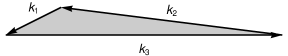
Figure 4: Example of an ‘elongated’ bispectrum momentum-vector triangle which can be produced from high-energy physics, where $k_{1}+k_{2}\approx k_{3}$.

III.4 High-Energy Correction B

The next diagram is very similar,

$$B_{\varphi}^{B} = \frac{(-ig_{1})(-i\lambda_{1})}{(2\pi)^{3}}\int^{0}_{\tau_{\rm in}}d\tau_{1}\ a(\tau_{1})^{4}\int^{0}_{\tau_{\rm in}}d\tau_{2}\ a(\tau_{2})^{4}\times$$

$$\int\frac{d^{3}{\bf q}}{(2\pi)^{3}}\Big{(}[-iG^{R}_{{\bf k}_{1}}(0,\tau_{1})]F_{{\bf k}_{2}}(0,\tau_{1})[-iG^{R}_{{\bf q}}(\tau_{1},\tau_{2})]\times$$

$$[-i\mathcal{G}^{R}_{{\bf q}-{\bf k}_{3}}(\tau_{1},\tau_{2})][-iG^{A}_{{\bf k}_{3}}(\tau_{2},0)]+\ {\rm permutations}\Big{)}.$$

We do not need to explicitly evaluate this, however, because in the stationary phase approximation this is easily seen to be identical to diagram A but with a minus sign and the Heaviside function $\theta(\tau_{1}-\tau_{2})$. This allows us to integrate over only half the fluctuations in $\tau_{1},\tau_{2}$ and hence we get

$$B_{\varphi}^{B}=-\frac{1}{2}B_{\varphi}^{A}.$$

III.5 High-Energy Corrections C and D

There are two additional diagrams from high-energy interactions,

$$B_{\varphi}^{C} = \frac{(-ig_{1})(-i\lambda_{1})}{(2\pi)^{3}}\int^{0}_{\tau_{\rm in}}d\tau_{1}\ a(\tau_{1})^{4}\int^{0}_{\tau_{\rm in}}d\tau_{2}\ a(\tau_{2})^{4}\times$$

$$\int\frac{d^{3}{\bf q}}{(2\pi)^{3}}\Big{(}[-iG^{R}_{{\bf k}_{1}}(0,\tau_{1})]F_{{\bf k}_{2}}(0,\tau_{1})[-iG^{R}_{{\bf q}}(\tau_{1},\tau_{2})]\times$$

$$\mathcal{F}_{{\bf q}-{\bf k}_{3}}(\tau_{1},\tau_{2})F_{{\bf k}_{3}}(\tau_{2},0)+{\rm permutations}\Big{)},$$

$$B_{\varphi}^{D} = \frac{(-ig_{1})(-i\lambda_{1})}{(2\pi)^{3}}\int^{0}_{\tau_{\rm in}}d\tau_{1}\ a(\tau_{1})^{4}\int^{0}_{\tau_{\rm in}}d\tau_{2}\ a(\tau_{2})^{4}\times$$

$$\int\frac{d^{3}{\bf q}}{(2\pi)^{3}}\Big{(}[-iG^{R}_{{\bf k}_{1}}(0,\tau_{1})]F_{{\bf k}_{2}}(0,\tau_{1})F_{{\bf q}}(\tau_{1},\tau_{2})\times$$

$$[-i\mathcal{G}^{R}_{{\bf q}-{\bf k}_{3}}(\tau_{1},\tau_{2})]F_{{\bf k}_{3}}(\tau_{2},0)+{\rm permutations}\Big{)}.$$

This time, the stationary phase approximation implies the total cancellation of these terms against each other. As first observed in the power spectrum calculation Jackson:2010cw , this is a general theme: the leading-order corrections arising from the dynamics effective action will cancel, and the dominant corrections by power counting arise entirely from the density matrix.

III.6 Total Bispectrum

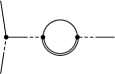
Figure 5: Examples of 3-point diagrams which are model-dependent, and so not considered here.

The complete bispectrum correction is then

$$B_{\varphi}=B_{\varphi}^{\rm self}+B_{\varphi}^{A}+B_{\varphi}^{B}.$$

The high-energy physics produces a scale-invariant elongated shape of bispectrum corrections.

There are a few other diagrams involving high-energy interactions shown in Figure 5, but they all involve a local or derivative coupling (strongly constrained by slow-roll), as well as a factor of $H/M$. Thus, these model-dependent terms will be subleading to the diagrams computed here. In non-slow roll models local terms may significantly contribute and in fact correspond precisely to the terms discussed in Meerburg:2009fi . The vacuum modification should also enhance local interactions, as first found in Ganc:2011dy ; Chialva:2011hc . Higher-derivative actions (for example, DBI Alishahiha:2004eh or more generally Chen:2006nt ) favor large equilateral bispectra Creminelli:2003iq , although will likely contain new features due to the high-energy physics.

IV Trispectrum Corrections

The 4-point correlation, or trispectrum, is defined analogously to the bispectrum:

$$T_{\varphi}({\bf k}_{1},{\bf k}_{2},{\bf k}_{3},{\bf k}_{4})(2\pi)^{3}\delta^{3}\left({\bf k}_{1}+{\bf k}_{2}+{\bf k}_{3}+{\bf k}_{4}\right)$$ (17)

$$\equiv \langle{\rm in}(0)|\varphi_{{\bf k}_{1}}(0)\varphi_{{\bf k}_{2}}(0)\varphi_{{\bf k}_{3}}(0)\varphi_{{\bf k}_{4}}(0)|{\rm in}(0)\rangle.$$

It was suggested in Jackson:2011qg that highly oscillatory corrections to power spectrum may be invisible, yet show up in the trispectrum as enhanced variance. This is because the dominant contribution to the trispectrum is the power spectrum-squared,

$$T_{\varphi}\sim\delta^{3}({\bf k}_{1}-{\bf k}_{2})\delta^{3}({\bf k}_{3}-{\bf k}_{4})P_{\varphi}(k_{1})P_{\varphi}(k_{3})+{\rm permutations}.$$

A modification in $P_{\varphi}$ of order $H/M$ would then produce a change of order $2P_{\varphi}H/M$ in $T_{\varphi}$. Below we will evaluate the corrections to $T_{\varphi}$, due to self- and high-energy interactions. We will see that this is not true.

IV.1 Self Interactions

Figure 6: Contributions to the trispectrum from self-interactions. There are also $\mathcal{O}(g_{0}^{2})$ and $\mathcal{O}(\lambda_{0}^{2})$ contributions which we can neglect in slow-roll inflation due to the strong constraints on the couplings.

The first non-factorizable contribution will be from the self-interaction as shown in Figure 6, again using a late-time cutoff $\mu\rightarrow 0^{-}$ and the most singular part of the exponential integral given by (8),

$$T_{\varphi}^{\rm self} = \frac{(-i\lambda_{0})}{(2\pi)^{3}}\int^{\mu}_{-\infty(1+i\epsilon)}d\tau\ a(\tau)^{4}\times$$

$$\Big{(}F_{{\bf k}_{1}}(0,\tau)F_{{\bf k}_{2}}(0,\tau)F_{{\bf k}_{3}}(0,\tau)[-iG^{R}_{{\bf k}_{4}}(0,\tau)]+\ {\rm permutations}$$

$$+F_{{\bf k}_{1}}(0,\tau)[-iG^{R}_{{\bf k}_{2}}(0,\tau)][-iG^{R}_{{\bf k}_{3}}(0,\tau)][-iG^{R}_{{\bf k}_{4}}(0,\tau)]$$

$$+\ {\rm permutations}\Big{)}$$

$$=\frac{i\lambda_{0}}{8(2\pi)^{3}(k_{1}k_{2}k_{3}k_{4})^{3/2}}\int^{\mu}_{-\infty(1+i\epsilon)}\frac{d\tau}{\tau^{4}}\times$$

$$\Big{[}U^{*}_{{\bf k}_{1}}(\tau)U_{{\bf k}_{2}}(\tau)U_{{\bf k}_{3}}(\tau)U_{{\bf k}_{4}}(\tau)+{\rm permutations}-{\rm c.c.}\Big{]}$$

$$\approx\frac{\lambda_{0}\mu^{-3}H^{4}}{24(2\pi k_{1}k_{2}k_{3}k_{4})^{3}}.$$

Such local trispectrum correlation functions clearly peaks at $k_{i}\approx 0$, and has been studied in Hu:2001fa . This has a non-linearity parameter $g_{\rm NL}^{\rm self}\sim T^{\rm self}_{\varphi}/P^{3}_{\rm\varphi}\sim k^{-3}$ scaling. There will also be corrections of order $T_{\varphi}\sim g_{0}^{2}H^{2}$ and $T_{\varphi}\sim\lambda_{0}^{2}H^{4}$, which are again presumed negligible from slow-roll constraints.

IV.2 Tree-Level High-Energy Corrections

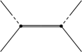
A

B

C

Figure 7: Tree-level high-energy contributions to the 4-point correlation function.

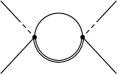
D

E

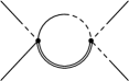
F

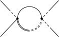
G

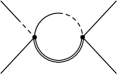
H

I

Figure 8: Loop high-energy contributions to the 4-point correlation function.

Figure 7 shows the three tree-level high-energy diagrams contributing to the trispectrum corrections. We first evaluate diagram A,

$$T_{\varphi}^{A} = \frac{(-ig_{1})^{2}}{(2\pi)^{3}}\int^{0}_{\tau_{\rm in}}d\tau_{1}\ a(\tau_{1})^{4}\int^{0}_{\tau_{\rm in}}d\tau_{2}\ a(\tau_{2})^{4}\times$$

$$\hskip 14.45377pt\Big{(}[-iG^{R}_{{\bf k}_{1}}(0,\tau_{1})]F_{{\bf k}_{2}}(0,\tau_{1})\mathcal{F}_{{\bf k}_{1}+{\bf k}_{2}}(\tau_{1},\tau_{2})\times$$

$$\hskip 21.68121pt[-iG^{A}_{{\bf k}_{3}}(\tau_{2},0)]F_{{\bf k}_{4}}(\tau_{2},0)+\ {\rm permutations}\Big{)}$$

$$= \frac{g_{1}^{2}H^{4}}{4(16\pi^{2}k_{1}k_{2}k_{3}k_{4})^{3/2}}\Big{[}\mathcal{A}_{1}({\bf k}_{1},{\bf k}_{2})\mathcal{A}_{1}^{*}({\bf k}_{3},{\bf k}_{4})+{\rm c.c.}\Big{]}$$

$$= \frac{g_{1}^{2}H^{3}}{2^{10}\pi^{2}(k_{1}k_{2}k_{3}k_{4})^{2}M}\times$$

$$\left[(k_{1}+k_{2})^{2}-|{\bf k}_{1}+{\bf k}_{2}|^{2}\right]^{-1/4}\left[(k_{3}+k_{4})^{2}-|{\bf k}_{3}+{\bf k}_{4}|^{2}\right]^{-1/4}\times$$

$$\left(\frac{k_{1}+k_{2}+\sqrt{(k_{1}+k_{2})^{2}-|{\bf k}_{1}+{\bf k}_{2}|^{2}}}{k_{3}+k_{4}+\sqrt{(k_{3}+k_{4})^{2}-|{\bf k}_{3}+{\bf k}_{4}|^{2}}}\right)^{-iM/H}+{\rm c.c.}$$

$$+ {\rm permutations.}$$

As in the bispectrum, the oscillating phase corresponds to the difference in interaction time between the two vertices. In this case, however, there is no loop-momentum integration to wash the oscillations out. That these oscillations are really present is in fact easy to understand. Due to the cosmological blueshift the difference in interaction times translates into a difference in energies. The Schwinger-Keldysh-Feynman diagram describes a coherent pair of heavy particles spontaneously created each separately decaying into light particles at different moments where the on-shell condition is reached. One can therefore effectively think of the heavy particle as a superposition of “two” states, $|\chi\rangle=\frac{1}{\sqrt{1+|\alpha|^{2}}}\left(|\chi_{1}\rangle+\alpha|\chi_{2}\rangle\right)$, one state $\chi_{1}$ which decays to $\chi_{1}\rightarrow\varphi(k_{1})+\varphi(k_{2})$, the other to $\chi_{2}\rightarrow\varphi(k_{3})+\varphi(k_{4})$. Moreover (though energy is not a good quantum number in cosmology) the effective energy encoded in the interaction time is different for $\chi_{1}$ and $\chi_{2}$. A state which is a superposition of two different energy states with respective energies $E_{1},E_{2}$ and lifetimes $\tau_{1},\tau_{2}$ famously shows oscillations in its time evolution:

$$|\langle\chi(t)|\chi(0)\rangle|^{2}=\frac{1}{(1+|\alpha|^{2})^{2}}\left(e^{-t/\tau_{1}}+|\alpha|^{2}e^{-t/\tau_{2}}\right.$$

$$\hskip 28.90755pt\left.+2|\alpha|e^{-t(\tau_{1}+\tau_{2})/2\tau_{1}\tau_{2}}\cos t(E_{2}-E_{1})\right).$$

This is what underlies e.g. neutrino oscillations. To emphasize that it is the same physics here, recall that

$$\sqrt{(k_{1}+k_{2})^{2}-|\mathbf{k_{1}}+\mathbf{k_{2}}|^{2}}=M/H|\tau_{12}|~{}.$$ (19)

Defining a physical energy similar to eqn (16),

$$E_{12}=(k_{1}+k_{2})H|\tau_{12}|,$$ (20)

$T_{\varphi}^{A}$ can be rewritten as

$$T_{\varphi}^{A} \sim \sqrt{\frac{M^{2}}{H^{2}\tau_{12}\tau_{34}}}\cos\left[\frac{M}{H}\ln\frac{(E_{12}+M)\tau_{34}}{(E_{34}+M)\tau_{12}}\right]$$

$$\sim \sqrt{\frac{M^{2}}{H^{2}\tau_{12}\tau_{34}}}\cos\left[\frac{M}{H}\ln\frac{\tau_{34}}{\tau_{12}}\right.$$

$$\hskip 28.90755pt\left.+\ln\left(1+\frac{E_{12}}{M}\right)-\ln\left(1+\frac{E_{34}}{M}\right)\right]$$

Approximating $\ln(1+E/M)=E/M+\ldots$ and transforming to cosmological time $\tau=-e^{-Ht}/H$,

$$T_{\varphi}^{A}\sim\sqrt{\frac{M^{2}}{H^{2}\tau_{12}\tau_{34}}}\cos\left[M(t_{12}-t_{34})+\frac{E_{12}}{H}-\frac{E_{34}}{H}\right]$$

$$\hskip 57.81621pt+\ \rm{permutations}$$ (21)

we recognize the familiar $\Delta E$ interference term with a new cosmological $\Delta t$ term as well. For the specific case $k_{1}+k_{2}=k_{3}+k_{4}$ the energy is conserved, making the vertex interaction time equal, and the oscillations disappear. This is also scale-invariant, $g^{A}_{\rm NL}\sim T^{A}_{\varphi}/P^{3}_{\varphi}\sim 1$. By combining such high-energy interactions with local ones, there would be an enhancement as seen in Agullo:2011aa .

To see whether these characteristic oscillatory features are present in the total signal, we must also compute the next two diagrams. They are

$$T_{\varphi}^{B} = \frac{(-ig_{1})^{2}}{(2\pi)^{3}}\int^{0}_{\tau_{\rm in}}d\tau_{1}\ a(\tau_{1})^{4}\int^{0}_{\tau_{\rm in}}d\tau_{2}\ a(\tau_{2})^{4}\times$$

$$\left[-iG^{R}_{{\bf k}_{1}}(0,\tau_{1})\right]F_{{\bf k}_{2}}(0,\tau_{1})\left[-i\mathcal{G}^{R}_{{\bf k}_{1}+{\bf k}_{2}}(\tau_{1},\tau_{2})\right]F_{{\bf k}_{3}}(\tau_{2},0)F_{{\bf k}_{4}}(\tau_{2},0)$$

$$\hskip 72.26999pt+\ {\rm permutations},$$

$$T_{\varphi}^{C} = \frac{(-ig_{1})^{2}}{(2\pi)^{3}}\int^{0}_{\tau_{\rm in}}d\tau_{1}\ a(\tau_{1})^{4}\int^{0}_{\tau_{\rm in}}d\tau_{2}\ a(\tau_{2})^{4}\left[-iG^{R}_{{\bf k}_{1}}(0,\tau_{1})\right]\times$$

$$F_{{\bf k}_{2}}(0,\tau_{1})\left[-i\mathcal{G}^{R}_{{\bf k}_{1}+{\bf k}_{2}}(\tau_{1},\tau_{2})\right]\left[-iG^{A}_{{\bf k}_{3}}(\tau_{2},0)\right]\left[-iG^{A}_{{\bf k}_{4}}(\tau_{2},0)\right]$$

$$\hskip 72.26999pt+\ {\rm permutations}.$$

Computing their effects, one easily sees that

$$T_{\varphi}^{B}=T_{\varphi}^{C}=-\frac{1}{2}T_{\varphi}^{A}.$$

The leading $H/M$ contribution therefore vanishes.

IV.3 Loop High-Energy Corrections

Now turning to the loop corrections in Figure 8, the first is

$$T_{\varphi}^{D} = \frac{(-i\lambda_{1})^{2}}{(2\pi)^{3}}\int^{0}_{\tau_{\rm in}}d\tau_{1}\ a(\tau_{1})^{4}\int^{0}_{\tau_{\rm in}}d\tau_{2}\ a(\tau_{2})^{4}\times$$

$$\int\frac{d^{3}{\bf q}}{(2\pi)^{3}}\Big{(}[-iG^{R}_{{\bf k}_{1}}(0,\tau_{1})]F_{{\bf k}_{2}}(0,\tau_{1})F_{{\bf q}}(\tau_{1},\tau_{2})\times$$

$$\mathcal{F}_{{\bf k}_{1}+{\bf k}_{2}+{\bf q}}(\tau_{1},\tau_{2})[-iG^{A}_{{\bf k}_{3}}(\tau_{2},0)]F_{{\bf k}_{4}}(\tau_{2},0)+{\rm perms.}\Big{)}$$

$$=\frac{\lambda_{1}^{2}H^{4}}{2\pi^{3}(k_{1}k_{2}k_{3}k_{4})^{3/2}}\times$$

$$\int\frac{d^{3}{\bf q}}{(2\pi)^{3}}\Big{[}\mathcal{B}_{1}({\bf k}_{1},{\bf k}_{2},{\bf q})\mathcal{B}_{1}^{*}({\bf k}_{3},{\bf k}_{4},{\bf q})+{\rm c.c.}+{\rm perms.}\Big{]}.$$

There is a rapidly-varying phase present completely analogous to (12),

$$\left(\frac{k_{1}+k_{2}+q+\sqrt{(k_{1}+k_{2}+q)^{2}-|{\bf k}_{1}+{\bf k}_{2}+{\bf q}|^{2}}}{k_{3}+k_{4}+q+\sqrt{(k_{3}+k_{4}+q)^{2}-|{\bf k}_{3}+{\bf k}_{4}+{\bf q}|^{2}}}\right)^{-iM/H}.$$

As in the bispectrum loop integration, the integration over ${\bf q}$ will only allow contributions near $k_{1}+k_{2}=k_{3}+k_{4}$. Now defining variables appropriate to this case,

$$\kappa_{12} \equiv k_{1}+k_{2}-(k_{3}+k_{4}),$$

$$u^{-1} \equiv -\sqrt{(k_{1}+k_{2}+q)^{2}-|{\bf k}_{1}+{\bf k}_{2}+{\bf q}|^{2}},$$

$$E \equiv Mq|u|.$$

Taking $\theta$ to be the angle between $k_{12}\equiv{\bf k}_{1}+{\bf k}_{2}$ and ${\bf q}$, the $(u,E)$ variables can be inverted to yield

$$q = \frac{E}{M|u|},$$

$$1-\cos\theta = \frac{M|u|}{2k_{12}E}\left[|u|^{-2}-(k_{1}+k_{2})^{2}+k_{12}^{2}\right].$$

Just as in the bispectrum case, the integral transforms as

$$\int\frac{d^{3}\bf q}{(2\pi)^{3}}\rightarrow-\frac{1}{(2\pi)^{2}M^{2}k_{12}}\int\frac{duEdE}{u^{5}}.$$ (22)

The integrand transforms as

$$\mathcal{B}_{1}({\bf k}_{1},{\bf k}_{2},{\bf q})\mathcal{B}_{1}^{*}({\bf k}_{3},{\bf k}_{4},{\bf q})\rightarrow\frac{\pi|u|^{4}M^{2}e^{-i\frac{M}{H}\kappa_{12}u}}{16HE\sqrt{k_{1}k_{2}k_{3}k_{4}}}+\mathcal{O}(\kappa_{12}).$$

The bounds are now

$$\frac{M|u|\left[|u|^{-2}+k_{12}^{2}-(k_{1}+k_{2})^{2}\right]}{2(k_{1}+k_{2}+k_{12})}\leq E\leq\Lambda-M(k_{1}+k_{2})|u|,$$

$$|u_{\pm}|=\frac{1}{\left(k_{12}+k_{1}+k_{2}\right)^{2}}\times$$

$$\left[\left(\frac{\Lambda}{M}\right)k_{12}\pm\sqrt{\left(\frac{\Lambda}{M}\right)^{2}k_{12}^{2}-\left(k_{12}+k_{1}+k_{2}\right)^{2}}\right].$$

The energy integral is again trivial, and expanding near the extremum at $|u_{0}|=M/\Lambda(k_{1}+k_{2}+k_{12})$ the resultant integrand can be approximated as Gaussian:

$$|u|^{-1}\Big{[}\Lambda-M(k_{1}+k_{2})|u|$$

$$\left.\hskip 36.135pt-\frac{M|u|\left[|u|^{-2}+k_{12}^{2}-(k_{1}+k_{2})^{2}\right]}{2(k_{1}+k_{2}+k_{12})}\right]$$

$$\approx \frac{\Lambda^{2}(k_{1}+k_{2}+k_{12})}{2M}\times$$

$$\exp\left[-\frac{1}{2}\left(\frac{\Lambda}{M}\right)^{2}(k_{1}+k_{2}+k_{12})^{2}(u-u_{0})^{2}\right].$$

Now performing the integral over $u$,

$$\int_{-\infty}^{\infty}du\ e^{-i\frac{M}{H}\kappa_{12}u-\frac{1}{2}\left(\frac{\Lambda}{M}\right)^{2}(k_{1}+k_{2}+k_{12})^{2}(u-u_{0})^{2}}+{\rm c.c.}$$

$$\approx \frac{\sqrt{2\pi}M}{\Lambda(k_{1}+k_{2}+k_{12})}e^{-i\frac{M}{H}\kappa_{12}u_{0}-\frac{1}{2}\left(\frac{M^{2}\kappa_{12}}{H\Lambda(k_{1}+k_{2}+k_{12})}\right)^{2}}+{\rm c.c.}$$

$$\approx \frac{4\pi H}{M}\delta(\kappa_{12}).$$

The final answer is then

$$T^{D}_{\varphi}=\frac{\pi\lambda_{1}^{2}H^{4}\Lambda^{2}(k_{1}+k_{2}+k_{12})}{(2\pi)^{4}M^{2}(k_{1}k_{2}k_{3}k_{4})^{2}k_{12}}\delta(k_{1}+k_{2}-k_{3}-k_{4})+{\rm perms.}$$ (23)

The $(\Lambda/M)^{2}$ can be absorbed into the bare coupling $\lambda_{1}$. Unlike the tree-level trispectrum corrections, there is no $H/M$ dependence in the magnitude of (23). Like the other high-energy diagrams calculated, it is scale-invariant.

The next diagram is similar,

$$T_{\varphi}^{E} = \frac{(-i\lambda_{1})^{2}}{(2\pi)^{3}}\int^{0}_{\tau_{\rm in}}d\tau_{1}\ a(\tau_{1})^{4}\int^{0}_{\tau_{\rm in}}d\tau_{2}\ a(\tau_{2})^{4}\times$$

$$\int\frac{d^{3}{\bf q}}{(2\pi)^{3}}\Big{(}[-iG^{R}_{{\bf k}_{1}}(0,\tau_{1})]F_{{\bf k}_{2}}(0,\tau_{1})[-iG^{R}_{{\bf q}}(\tau_{1},\tau_{2})]\times$$

$$\mathcal{[}-iG^{R}_{{\bf k}_{1}+{\bf k}_{2}+{\bf q}}(\tau_{1},\tau_{2})][-iG^{A}_{{\bf k}_{3}}(\tau_{2},0)]F_{{\bf k}_{4}}(\tau_{2},0)+{\rm perms.}\Big{)}.$$

It is easy to see that $T^{E}_{\varphi}=-\frac{1}{2}T^{D}_{\varphi}$. Using the formula for $u_{c}$ in the $\mathcal{B}$’s, we assume that $k_{1}+k_{2}\geq k_{3}+k_{4}$ to ensure $u_{1}\geq u_{2}$.

Finally, $T_{\varphi}^{F}$ and $T_{\varphi}^{G}$ cancel, and $T_{\varphi}^{H}$ and $T_{\varphi}^{I}$ cancel.

IV.4 Total Trispectrum

Taking advantage of the cancellations between several diagrams, the total trispectrum is

$$T_{\varphi} = (2\pi)^{6}\delta^{3}({\bf k}_{1}-{\bf k}_{2})\delta^{3}({\bf k}_{3}-{\bf k}_{4})P_{\varphi}(k_{1})P_{\varphi}(k_{3})$$

$$+{\rm permutations}+T^{\rm self}_{\varphi}+T_{\varphi}^{D}+T_{\varphi}^{E}.$$

While oscillations arise at order $H/M$ in individual diagrams, their cancellation means that no such feature appears in the final result.

V Conclusion

We have computed the generic primordial bi- and trispectrum corrections in an inflating background due to high energy physics. The dominant physics arises from the New Physics Hypersurface where the cosmological blueshift can just create an on-shell heavy particle. As predicted Holman:2007na ; Meerburg:2009ys ; Meerburg:2009fi , the bispectrum corrections peak near the elongated shape of momentum-triangle; here we derive this ab initio. The bispectrum otherwise contains no extraordinary features. The trispectrum has no leading order effect. Even though the interference effect of the effective mass-shell-time-difference for a pair of heavy particles, similar to neutrino oscillations, this cancels when all diagrams are taken into account.

Like that of the power spectrum, the magnitude of the bispectrum high-energy corrections are estimated to be of order $H/M$. For optimistic but not impossible values of $H/M\sim 0.01$ these corrections could possibly be measured by Planck planck and other precision experiments in the near future. Also like the power spectrum, the leading corrections arising from the dynamical part of the effective action cancel and the dominant corrections arise entire from the density matrix.

We emphasize that we have only calculated the model-independent corrections. Specific models will no doubt produce very rich features and should be studied in more detail.

VI Acknowledgments

We would like to thank F. Bouchet, J. Fergusson, E. Komatsu, and B. Wandelt for discussions. This research was supported in part by a VIDI and a VICI Innovative Research Incentive Award from the Netherlands Organisation for Scientific Research (NWO), a van Gogh grant from the NWO, and the Dutch Foundation for Fundamental Research on Matter (FOM).

References

- (1)
- (2) A. H. Guth, “The Inflationary Universe: A Possible Solution To The Horizon And Flatness Problems,” Phys. Rev. D 23, 347 (1981).
- (3) A. D. Linde, “A New Inflationary Universe Scenario: A Possible Solution Of The Horizon, Flatness, Homogeneity, Isotropy And Primordial Monopole Problems,” Phys. Lett. B 108, 389 (1982).
- (4) A. Albrecht and P. J. Steinhardt, “Cosmology For Grand Unified Theories With Radiatively Induced Symmetry Breaking,” Phys. Rev. Lett. 48, 1220 (1982).
- (5) A. D. Linde, “Chaotic Inflation,” Phys. Lett. B 129, 177 (1983).
- (6) R. H. Brandenberger, “Inflationary cosmology: Progress and problems,” arXiv:hep-ph/9910410.
- (7) B. Greene, K. Schalm, J. P. van der Schaar and G. Shiu, “Extracting new physics from the CMB,” In the Proceedings of 22nd Texas Symposium on Relativistic Astrophysics at Stanford University, Stanford, California, 13-17 Dec 2004, pp 0001 [arXiv:astro-ph/0503458].
- (8) E. Komatsu et al. [WMAP Collaboration], “Seven-Year Wilkinson Microwave Anisotropy Probe (WMAP) Observations: Cosmological Interpretation,” arXiv:1001.4538 [astro-ph.CO]; D. Larson et al. [WMAP Collaboration], “Seven-Year Wilkinson Microwave Anisotropy Probe (WMAP) Observations: Power Spectra and WMAP-Derived Parameters,” arXiv:1001.4635 [astro-ph.CO].
- (9) [Planck Collaboration], “Planck: The scientific programme,” arXiv:astro-ph/0604069.
- (10) “Euclid: Mapping the geometry of the dark universe”, Assessment Report by the ESA, December 2009.
- (11) D. Baumann, M. G. Jackson et al. [ CMBPol Study Team Collaboration ], “CMBPol Mission Concept Study: Probing Inflation with CMB Polarization,” AIP Conf. Proc. 1141, 10-120 (2009). [arXiv:0811.3919 [astro-ph]]; D. Baumann et al. [CMBPol Study Team Collaboration], “CMBPol Mission Concept Study: A Mission to Map our Origins,” AIP Conf. Proc. 1141, 3 (2009) [arXiv:0811.3911 [astro-ph]].
- (12) E. Komatsu et al., “Non-Gaussianity as a Probe of the Physics of the Primordial Universe and the Astrophysics of the Low Redshift Universe,” arXiv:0902.4759 [astro-ph.CO].
- (13) A. P. S. Yadav and B. D. Wandelt, “Evidence of Primordial Non-Gaussianity (f(NL)) in the Wilkinson Microwave Anisotropy Probe 3-Year Data at 2.8sigma,” Phys. Rev. Lett. 100, 181301 (2008) [arXiv:0712.1148 [astro-ph]].
- (14) L. Senatore, K. M. Smith and M. Zaldarriaga, “Non-Gaussianities in Single Field Inflation and their Optimal Limits from the WMAP 5-year Data,” JCAP 1001, 028 (2010) [arXiv:0905.3746 [astro-ph.CO]].
- (15) E. Komatsu and D. N. Spergel, “Acoustic signatures in the primary microwave background bispectrum,” Phys. Rev. D 63, 063002 (2001) [arXiv:astro-ph/0005036].
- (16) P. Creminelli, “On non-Gaussianities in single-field inflation,” JCAP 0310, 003 (2003) [arXiv:astro-ph/0306122].
- (17) M. Alishahiha, E. Silverstein and D. Tong, “DBI in the sky,” Phys. Rev. D 70, 123505 (2004) [arXiv:hep-th/0404084].
- (18) R. Holman and A. J. Tolley, “Enhanced Non-Gaussianity from Excited Initial States,” JCAP 0805, 001 (2008) [arXiv:0710.1302 [hep-th]].
- (19) P. D. Meerburg, J. P. van der Schaar and P. S. Corasaniti, “Signatures of Initial State Modifications on Bispectrum Statistics,” JCAP 0905, 018 (2009) [arXiv:0901.4044 [hep-th]].
- (20) P. D. Meerburg, J. P. van der Schaar and M. G. Jackson, “Bispectrum signatures of a modified vacuum in single field inflation with a small speed of sound,” JCAP 1002, 001 (2010) [arXiv:0910.4986 [hep-th]].
- (21) X. Chen, “Folded Resonant Non-Gaussianity in General Single Field Inflation,” JCAP 1012, 003 (2010) [arXiv:1008.2485 [hep-th]].
- (22) J. Ganc, “Calculating the local-type fNL for slow-roll inflation with a non-vacuum initial state,” Phys. Rev. D 84, 063514 (2011) [arXiv:1104.0244 [astro-ph.CO]].
- (23) D. Chialva, “Signatures of very high energy physics in the squeezed limit of the bispectrum from the field theoretical approach,” arXiv:1108.4203 [astro-ph.CO].
- (24) J. R. Fergusson, M. Liguori and E. P. S. Shellard, “The CMB Bispectrum,” arXiv:1006.1642 [astro-ph.CO].
- (25) M. G. Jackson and K. Schalm, “Model Independent Signatures of New Physics in the Inflationary Power Spectrum,” Phys. Rev. Lett. 108, 111301 (2012) [arXiv:1007.0185 [hep-th]].
- (26) M. G. Jackson and K. Schalm, “Model-Independent Signatures of New Physics in Slow-Roll Inflation,” arXiv:1104.0887 [hep-th].
- (27) M. G. Jackson, “Integrating out Heavy Fields in Inflation,” arXiv:1203.3895 [hep-th].
- (28) E. Calzetta and B. L. Hu, “Nonequilibrium Quantum Fields: Closed Time Path Effective Action, Wigner Function and Boltzmann Equation,” Phys. Rev. D 37, 2878 (1988).
- (29) T. S. Bunch and P. C. W. Davies, “Quantum Field Theory In De Sitter Space: Renormalization By Point Splitting,” Proc. Roy. Soc. Lond. A 360, 117 (1978).
- (30) J. M. Maldacena, “Non-Gaussian features of primordial fluctuations in single field inflationary models,” JHEP 0305, 013 (2003) [arXiv:astro-ph/0210603].
- (31) X. Chen, M. x. Huang, S. Kachru and G. Shiu, “Observational signatures and non-Gaussianities of general single field inflation,” JCAP 0701, 002 (2007) [arXiv:hep-th/0605045].
- (32) E. Sefusatti, M. Liguori, A. P. S. Yadav, M. G. Jackson and E. Pajer, “Constraining Running Non-Gaussianity,” JCAP 0912, 022 (2009) [arXiv:0906.0232 [astro-ph.CO]].
- (33) W. Hu, “Angular trispectrum of the CMB,” Phys. Rev. D 64, 083005 (2001) [astro-ph/0105117].
- (34) I. Agullo, J. Navarro-Salas and L. Parker, “Enhanced local-type inflationary trispectrum from a non-vacuum initial state,” arXiv:1112.1581 [astro-ph.CO].