Protocol Coding through Reordering of User Resources, Part II: Practical Coding Strategies

Abstract

We use the term protocol coding to denote the communication strategies in which information is encoded through the actions taken by a certain communication protocol. In this work we investigate strategies for protocol coding via combinatorial ordering of the labelled user resources (packets, channels) in an existing, primary system. This introduces a new, secondary communication channel in the existing system, which has been considered in the prior work exclusively in a steganographic context. Instead, we focus on the use of secondary channel for reliable communication with newly introduced secondary devices, that are low-complexity versions of the primary devices, capable only to decode the robustly encoded header information in the primary signals. In Part I of the work we have characterized the capacity of the secondary channel through information–theoretic analysis. In this paper we consider practical strategies for protocol coding inspired by the information–theoretic analysis. It turns out that the insights from Part I are instrumental for devising superior design of error–control codes. This is demonstrated by comparing the error performance to the “naïve” strategy which is presumably available without carrying out the analysis in Part I. These results are clearly outlining both the conceptual novelty behind the discussed concept of secondary channel as well as its practical applicability.

I Introduction

A way to introduce new features and define a new communication channel over an existing wireless system, without introducing hardware/physical layer changes, is to encode information in the actions take by the protocol of the existing (primary) communication system. We denote such a class of communication strategies by the term protocol coding. In this work we are considering a particular type of protocol coding, in which information is encoded in the ordering of labelled resources (packets, channels) of the primary (legacy) users. For example, if in a given scheduling frame the primary system decides to send $3$ packets to Alice and $2$ packets to Bob, then the secondary transmitter gets the right to encode additional information by rearranging these packets. This can be done in $\binom{5}{2}=10$ different ways, such that in that scheduling frame the secondary transmitter can send $\log_{2}10$ bits. In this example, a scheduling frame contains $F=5$ packets and the primary decides the state of the frame (how many packets to Alice and Bob, respectively). In each state there are different number of possible rearrangements and the problem is that the state is not controlled by the secondary, which means that the amount of information that the secondary can send it variable and unpredictable.

The restriction that stems from operation of the primary is the key feature of the communication model. In Part I [1] we have elaborated on the capacity of the model by using a framework where the secondary communication channel was represented through a cascade of channels. Such a framework is alternative to a rather standard representation using Shannon’s model of channels with causal channel state information at the transmitter (CSIT), but very potent in our case as we have been able to compute the secondary capacity under quite general error model assumptions. The capacity calculation has lead to the concept of a multisymbol, which is a set of actual packet rearrangements that represent identical secondary input symbol.

In practice, a secondary channel can be defined over virtually any existing wireless system and it is of interest to find the coding strategies that are suited to a certain primary system. We can ask the following question: If we did not have the capacity derivation and the multisymbol framework that has emerged from it, described in  [1], what would be the “naïve” way to design a code in order to communicate over the secondary channel? Conversely, what does the information–theoretic strategy developed in the Part I of the paper teach us about designing good codes (signaling) strategies for this channel?

In the absence of the multisymbol framework, we can perform the encoding in the traditional way, by taking any usual error-correcting code and an interleaver. However, a problem arises when we attempt to send a sequence of $F$ bits over the secondary channel of frame length $F$, which is in a given state $s$ which we do not control. If the sequence of bits we need to transmit is not one of the $\binom{F}{s}$ possible symbols, we should pick any (e. g. randomly) of the possible symbols which are at the same (minimal) Hamming distance from the bit sequence. For example, for a frame length $F=4$ we take four of the coded and interleaved bits and look at the current state of the channel (how many 1s we can transmit in the next frame). Then, we pick any (e. g. randomly) of the possible frames, obtained by permuting the packets, that has minimal possible Hamming distance. For example, when the system needs to transmit $0101$ and the state is $s=3$, it chooses randomly between $0111$ and $1101$. However, this leads to ambiguity since the receiver might falsely interpret the transmitted sequence as $0111$ being or $1101$, instead of $0101$. Hence, even when the channel does not introduce errors, there will be decoding errors.

Therefore, we have to look at other strategies which are applicable in the context of protocol coding. Besides its’ role in the capacity calculation, it turns out that the multisymbol framework can be used in the construction of error-correcting codes for secondary communication, since it gives an insight in the coding strategies that are approaching the capacity.

The rest of the paper is organized as follows. In Section II we present transmit strategies for the errorless case, i.e. the case when the probability of error for secondary reception is 0. In Section III we address the case of secondary communication when errors are present. First we investigate a naïve strategy for communication, which does not account for the specifics of secondary communication channels. Then, we propose a coding strategy which is inspired from the capacity results derived in Part I of the paper. In Section IV we present a trellis coding scheme where the trellis code is based on the multisymbol framework and evaluate its’ performance. Section V presents some distinguished features of secondary channels, potential applications and provides a discussion on the the limitations of the presented model for protocol coding. Finally, Section VI concludes the paper and gives directions for future work.

II Coding for Errorless Channels

II-A Motivation and System Model

In this section we introduce practical encoding strategies when the secondary channel is assumed errorless i. e. the headers (labels) of the primary packets are perfectly received at the secondary receiver. This is interesting, since using fixed-length codes necessarily leads to nonzero probability of error, despite the fact that there are no channel induced errors on the packet headers, which in turn cary the packet label, used for secondary communication. To see why this is the case, consider the example of a primary system with a scheduling frame with $F$ packets. Assume that one wants to encode secondary information by using $L$ consecutive frames. However, if the primary system decides the state to be $0$ in all frames (i. e. all the packets are addressed to Alice), then no secondary information can be encoded, which leads to error.

We consider a simplified model by having only two possible packet labels, i. e. each packet in a frame is addressed either to user $0$ or user $1$. This setup is sufficient to illustrate the main strategies for protocol coding with resource ordering. We recall that the set of packets that are scheduled in a frame is decided by the primary system, i.e. the secondary communication is restricted and can only rearrange the set of packets selected by the primary. The state of the frame $s$ is the number of packets addressed to user $1$ and occurs with probability $P_{S}(s)=\frac{\binom{F}{s}}{2^{F}}$. In the errorless case, the state $s$ is known to both the transmitter and the receiver. Thus, each state $s$ is associated with one communication sub-channel with a capacity $r(F,s)=\log_{2}\binom{F]}{s}$, as elaborated in Part I. In a given frame, the primary chooses the state $S=s$ with probability $P_{S}(s)$, independently of the states in the previous frames .

Let us consider $n$ frames, where each frame is a secondary channel use and let $s^{n}$ be the vector that describes the random outcome from observing the $n$ frames. As $n$ goes to infinity, the sequence $s^{n}$ becomes typical, such that the number of states that will have the value $s$ is approximately $\approx nP_{S}(s)$. The capacity of the the errorless channel can be calculated [2]:

$$C_{F,0}=\sum_{s=0}^{F}P_{S}(s)\log_{2}\binom{F}{s}$$ (1)

A scheme that achieves this capacity would work as follows. Consider transmission of a large message by using large number of channel uses $n\rightarrow\infty$. The sender segments the message into sub-messages, where each of the sub-messages is sent over a separate sub-channel (state), which occurs with probability $P_{S}(s)$. The sub-message that is to be sent over the sub-channel defined by $s$ contains approximately $nP_{S}(s)r_{(}F,s)$ bits. If during the $i-$th channel use the sender observes that the state $s$, then it takes the next $r(F,s)$ bits from the corresponding sub-message. Thus, the whole message is sent by time–interleaving of all the available sub–channels.

Nevertheless, in this paper we are focused on practical coding strategies and this scheme might be ineffective when sending messages of finite, short length $m$. For example, when the number of channel uses $n$ is finite, some of the channel states might not appear at all. In this case, the above strategy would fail to send a part of the message, i.e. the sub-messages associated with those states. What we need is a practical coding scheme which is tailored to the observation that the secondary system does not have a control over the state $s$ of the channel.

II-B Coding with Variable Radix

Since using a fixed-length secondary coding block introduces errors, we need to send a group of $m$ bits by using multiple (variable) number of frames, where the number of frames to be used depends on the realization of the sequence of channel states. We introduce the proposed coding strategy by taking an example with frame of length $F=4$.

II-B1 Example

Let us group the input bits into groups of size $m=10$ and let us call such a group of bits input symbol. Hence, one input symbol is a number between 0 and 1023. This input symbol will be sent by using several frames. Let the input symbol be the binary representation of $777$, for example. Let $s_{i}$ be the channel state in the $i-$th frame and let us assume the following state sequence $s_{1},s_{2},s_{3},s_{4},s_{5},s_{6}\cdots=2,3,0,2,1,3,\cdots$

The first state allows for $\binom{4}{2}=6$ different combinations. We divide the interval of integers $[0-123]$ in $6$ bins such that $4$ bins have a size of $171$ and $2$ bins have a size of $170$. The bins (sub-intervals) are given as $[0-170]$, $[171-341]$, $[342-512]$, $[513-683]$, $[684-853]$ and $[854-1023]$. The number $777$ is in the bin $5$. If we enumerate the $6$ possible combinations of packets when the state is $s=2$ as $0011,0101,0110,1001,1010,1100$, $5$ corresponds to the combination $1010$. Hence, Alice arranges the two packets in the frame and sends $1010$ in order to signal that the number $777$ is in the bin number $5$. When Bob receives the first frame and sees that $s_{1}=2$, then $B$ knows that it should use $6$ bins. In this way it gets the information that the number $M$ is in the $5$-th bin, $M\in[684-853]$.

Now Alice will use the subsequent frames in order to specify where within the bin $[684-853]$ is the number represented by the $m=10$ bits. For the second frame, the state is $s_{2}=3$. The number of possible packet rearrangements is $\binom{4}{3}=4$. Therefore, the bin $[684-853]$ is divided into $4$ sub-bins, such that $2$ bins have size of $43$ and $2$ bins have size of $42$. The bins are given as $[684-726],[727-769],[770-811]$ and $[812-853]$. Since $M=777$ belongs to the third bin, $M\in[770-811]$ and $s=3$, in the second frame we choose the packet rearrangement $1101$. Now, Bob knows that the transmitted number lies in the bin $[770-811]$.

When the third frame arrives, $s_{3}=0$ and no information can be sent by using combinatorial reordering.

We proceed in the same way for the rest of the frames. During the fourth frame the channel state is $s_{4}=2$, which allows for $6$ different combinations, i.e the bin $[770-811]$ is divided into $6$ sub-bins. Since $M=777$ belongs to the second bin, $M\in[777-783]$, we send the combination (rearrangement) $0101$. During the fifth frame the channel state is $s_{5}=1$, which allows for $4$ different combinations, i.e there are $4$ sub-bins. Since $M=777$ belongs to the first bin, $M\in[777-783]$, we send the combination (rearrangement) $0001$. During the sixth frame the channel state is $s_{6}=3$, which allows for $4$ different combinations. We divide the bin $[777-783]$ in $4$ sub-bins, given as $[777-778],[779-780],[781-782],[783]$. Since $M=777$ belongs to the first bin, $M\in[777-783]$, we send the combination (rearrangement) $0001$. Bob sees that the channel state is $s_{5}=1$, and knows that there are $4$ bins and that $M\in[777-778]$. This is over-dimensioned for the two bins we have left. Nevertheless, Alice can send $0011$ in order to inform Bob that the number is $M=777$.

Alternatively, Alice can apply additional optimization. Since $s_{6}=3$, the representation of the numbers in the bin $[777,778]$ is overprovisioned. Since the fourth frame can have $4$ possible combinations, it means that it can represent the $2$ possible numbers in the bin and also $2$ possible bins for the next input symbol. Let the next input symbol be $233$. We divide the interval $[0,1023]$ in $4$ bins, such that the $4$ bins have a size of $256$. Hence, the number $233$ is in bin $1$. This bin can be sent jointly with the last bin of the first input symbol. Now the interval $[1-4]$ is divided into $2$ bins of size $1$: $[1-2],[3-4]$. A needs to use the first bin, since $777$ is the first number in the uncertainty window $[777,778]$ for the first input symbol, but it will send the combination number $3$ (0110) in order to inform that $233$ is in the second bin of $1024$ when $1024$ is divided in $4$ bins as described above.

We note that for a different channel state sequence, the number of frames over which the coding was performed would differ. Hence, we speak of a variable-radix scheme which uses a variable number of frames to represent the secondary information bits. The variable radix scheme provides an effective mapping of the information bits into symbols, taking into account that the communication takes place over a multiple-state channel. Indeed, without having control of the channel state $s$, we can not send the sequence of information bits by using a single frame of length $F$ as the number of different combinations $\binom{F}{s}$ may not be sufficient. On the other hand, by taking multiple frames and allowing the number of frames to vary, this is always possible, as shown in the example. In this sense we can think of this scheme as an efficient modulation scheme, since it primarily provides mapping of the information bits into symbols, by taking into account the unpredictable channel states.

The example described above should be sufficient for the reader to devise variable-radix schemes for another state sequence. The problem with the variable-radix scheme is that it works only under perfect, errorless conditions and in the next section we discuss the practical strategies for protocol coding that can deal with channel -induced errors.

III Coding for Channels with Errors

As already argued, the variable-radix scheme fails in the presence of channel errors and might lead to catastrophic behavior. For example, if the channel is mostly errorless, but one symbol is in error, then the receiver Bob will not know where the current symbol ends and where the next starts, such that the whole sequence of information bits will be in error.

With this argument on mind, in the case with channel errors we would prefer to code over a fixed number of frames (and thus allow errors even when there are no channel-induced errors on the packet labels). The question is which coding strategy would be applicable in this case. We first look at a naïve coding strategy which does not account for the specifics of the secondary channel. Later, we present a communication scheme which is inspired by the capacity results derived previously

III-A Naïve Coding Strategy

The naïve strategy works as follows. We take any usual error-correction code of rate $R$ and interleave the output of this code, e.  g. by using a pseudo-random interleaver. The motivation for using an interleaver is to break the burst bit errors that can occur within one secondary symbol (frame). For example, for a frame length $F=4$ we take four of the coded and interleaved bits and look at the current state of the channel (how many 1s we can transmit in the next frame). Then, we pick any (e. g. randomly) of the possible frames, obtained by permuting the packets, that has minimal possible Hamming distance. For example, let the coded bits are 0101 and let the state be $s=3$. Then the Hamming distance of the “true information” 0101 from 0111, 1101 is 1 (minimal possible), while it is 3 from 1011 or 1110. Hence, when the system needs to transmit 0101 and the state is $s=3$, it chooses randomly between 0111 and 1101.

The trouble with the described naïve strategy is that, even when the channel does not introduce errors, there will be decoding errors. Additionally, as we will see in Section IV, the naïve strategy has poor performance in channels with transmission errors.

III-B Coding Strategy inspired from the Information–Theoretic Analysis

Here we propose a coding strategy which is inspired by the capacity results for the secondary communication channel derived in Part I. We start by recalling that we modelled the secondary communication channel by using a cascade of two channels $T-\mathbf{X}-\mathbf{Y}$ where the input constraints from the primary system were reflected in the way the set ${\cal P}_{\mathbf{X}|T}$ is defined. Then, instead of speaking about which strategies out of ${\cal T}$ that are chosen with non–zero probability, we speak of which representatives to choose for given secondary input symbol $T=t$. According to this, we introduced the notion of multisymbol, which is the set of representatives $\mathcal{M}_{t}=\{\mathbf{x}_{s}(t)\}$ for given $t$. Further, a minimal multisymbol was defined as a multisymbol obtained by permutation of the basic multisymbol, where the basic multisymbol has representatives defined as follows:

$$x_{s}(t)=\left\{\begin{array}[]{rl}0&\text{if }i\leq F-s\\ 1&\text{otherwise }\end{array}\right.$$

The minimal multisymbols satisfy the following Hamming distance relation $d_{H}(\mathbf{x}_{s}(t),\mathbf{x}_{s+1}(t))=1$ for each $s=0\ldots F-1$. The main capacity result for the secondary channel obtained in Part I has been stated in the following form

$$C\leq C_{XY}-I_{m}.$$

The term $C_{XY}$ is the capacity of the $\mathbf{X}-\mathbf{Y}$ channel, given by (12) in Part I. We recall that this capacity is attained by the distribution $\sum_{\mathbf{x}\in{\cal X}_{s}}P_{\mathbf{X}}(\mathbf{x})=P_{S}(s)$ and is upper bounded by the capacity of the channel defined by the underlying error model. $I_{m}$ is the minimal value (constant) of $I(\mathbf{X};\mathbf{Y}|T=t)$, achieved by the choice of the multisymbol as a minimal multisymbol. The equality is achieved if and only if there is a pair of distributions $\left(P_{T}(\cdot),P_{\mathbf{X}|T}(\cdot)\right)$ that simultaneously attains the maximum and the minimum in the first and the second term, respectively.

This result is quite general and holds for all classes of memoryless channels $\mathbf{X}-\mathbf{Y}$ with binary inputs. Among other channels, it holds for the erasure channel, the binary symmetric channel and the $Z$ channel. It has been further shown that for a uniform distribution over ${\cal T}$, this capacity can be achieved by a set $\mathcal{T}$ of cardinality $L=\textrm{lcm}\left(\binom{F}{0},\binom{F}{1},\ldots,\binom{F}{F}\right)$. The $L$ multisymbols should be minimal, meaning that the Hamming distance between two adjacent symbols is 1, $d_{H}(x_{s},x_{s+1})=1$.

From the viewpoint of capacity, the choice of the multisymbols is irrelevant, as long they are minimal and the distribution of $X$ fulfills the required condition. However, the choice of the multisymbols does affect the performance of the error-correcting code constructed based on the multisymbol framework.

Our aim is to use the multisymbol framework in the construction of practical coding schemes which are better suited for the secondary communication channel than the naïve approach. The question to ask is which criterion, e.g. distance metric we are going to use in the selection of the multisymbols. We adopt a heuristic approach and take the expected Hamming distance as the metric of interest for the choice of the $L$ multisymbols. The expected Hamming distance for two multisymbols $t_{1}$ and $t_{2}$ is defined as follows

$$E_{d_{H}}(t_{1},t_{2})=\sum_{s=0}^{F}P_{S}(s)d_{H}(x_{s}(t_{1}),x_{s}(t_{2})),$$ (2)

where $d_{H}$ is the Hamming distance between the two vectors. Clearly, considering the triviality of the states $s=0$ and $s=F$, we can simplify to:

$$E_{d_{H}}(t_{1},t_{2})=\sum_{s=1}^{F-1}P_{S}(s)d_{H}(x_{s}(t_{1}),x_{s}(t_{2}))$$ (3)

The motivation behind this is that this metric incorporates the state of the channel which can not be controlled by the secondary system.

With this in mind, we can construct a convolutional code by using the multisymbols framework and the expected Hamming distance as design criterion. We define a trellis for the convolutional code with a certain number of states. In the trellis diagram, each state contains two outgoing paths, each of them corresponding to one possible input binary symbol. Also, each state has two incoming paths. Each branch in the trellis is associated with an input symbol and an output symbol. In our case, the input symbol is binary and the output symbol is one of the $L$ multisymbols. The trellis is chosen on purpose to have $L$ branches, such that each multisymbol is used only once.

Now, the question is how we associate multisymbols with the transitions in the trellis. We use the known rules from trellis coding: the output symbols on the branches exiting from the same state should be maximally separated in terms of the expected Hamming distance. The same is valid for the output symbols associated with the two branches that enter the same state. In order to illustrate the code construction, we take the example with $F=4$, where the minimal cardinality of the uniform auxiliary variable $T$ is $L=\mathrm{lcm}\{\binom{4}{0},\binom{4}{1},\ldots,\binom{4}{4}\}=12$.

There are multiple ways in which the multisymbols can be chosen, and different sets have different features. We can get useful insights about the expected Hamming distance spectrum if we use the representation of the multisymbols as paths in the directed graph, as shown in Fig. 1. In order to maximize the expected Hamming distance between multisymbols, the paths corresponding to the multisymbols should be as diverse as possible. To assure this, we have to choose the multisymbols such to avoid (as much as possible) having multisymbols with common edges. Indeed, for two different multisymbols $t_{1}$ and $t_{2}$ which share a common edge $(x_{j}(t),x_{j+1}(t))$, the terms in the expected Hamming distance

$$E_{d_{H}}(t_{1},t_{2})=\sum_{s=0}^{F}P(S=s)d_{H}(x_{s}(t_{1}),x_{s}(t_{2})),$$ (4)

associated with that edge will be $0$. The necessary condition to avoid a common edge between the nodes from $\mathcal{X}_{s}$ and $\mathcal{X}_{s+1}$, where $s\leq\lfloor F/2\rfloor-1$, is that $L/\binom{F}{s}\leq F-s$. In other words, the edge weight should be at most $1$.

We note once again that the relevance of the expected Hamming distance as a performance metric is stated as a conjecture which is not rigorously proved. Moreover, one has to look at the whole distance spectrum, in order to be able to predict the performance of the error-correcting code. Since in the general case it is difficult to control the code distance spectrum, we turn to the the minimal expected Hamming distance as a simplified indicator of the code performance. However, in this particular case we have to be careful when making conclusions about the performance which are based solely on the minimal distance. As we are going to see in the next section, some of the simulation results indicate that the minimal expected Hamming distance is not the only factor which is decisive for the error performance.

In the following we give three representative examples of the set of multisymbols $\mathcal{T}$, created for $F=4$.

III-B1 Choice of multisymbols, Example 1

In the first example, we choose the $12$ multisymbols as given in Fig. 1 a). The multisymbols are chosen as a permutation of the basic multisymbol $\mathcal{M}_{b}=\{0000,0001,0011,0111,1111\}$ and fulfill the required property about the distribution of $X$. Hence, this choice is capacity achieving, but we need to investigate its performance in terms of error rate when used to construct a channel code. We use the representation of the multisymbols as paths in the directed graph, as shown in Fig. 1 b). We note that in the graph representation, some of the multisymbols have common edges which can be avoided. This, for example, is the case with the multisymbols $t_{1}=\{0000,0001,0011,0111,1111\}$ and $t_{4}=\{0000,0010,0011,0111,1111\}$. The expected Hamming distance profile for the above choice of the set of multisymbols reveals that the minimal distance is $0.5$.

$t$	$\{\mathbf{x}_{s}(t)\}$
$1$	$(0000,0001,0011,0111,1111)$
$2$	$(0000,0001,0101,1101,1111)$
$3$	$(0000,0001,1001,1011,1111)$
$4$	$(0000,0010,0011,0111,1111)$
$5$	$(0000,0010,1010,1011,1111)$
$6$	$(0000,0010,1010,1110,1111)$
$7$	$(0000,0100,0101,1101,1111)$
$8$	$(0000,0100,0110,0111,1111)$
$9$	$(0000,0100,0110,1110,1111)$
$10$	$(0000,1000,1001,1011,1111)$
$11$	$(0000,1000,1100,1101,1111)$
$12$	$(0000,1000,1100,1110,1111)$

(a)

(b)

Figure 1: Selection of the representative sets for $F=4$, Example 1. The selection of the multisymbols is not optimal. (a) Multisymbols for the $12$ inputs. (b) Graph representation of the process for selecting the multisymbols $\mathbf{x}_{s}(t)$.

III-B2 Choice of multisymbols, Example 2

In the second example, we choose the $12$ multisymbols as given in Fig. 2 a). We observe that no two multisymbols are identical and the choice of the multisymbols is capacity achieving. The graph used for selection of the multisymbols is shown in Fig. 2 c). The multisymbols are constructed by using each edge of the graph exactly once, except for the edges between $\mathcal{X}_{0}=\{0000\}$ and $\mathcal{X}_{1}=\{0001,0010,0100,1000\}$, where common edges can not be avoided. Additionally, common edges are avoided later in the graph, by an adequate choice of the paths associated with the multisymbols. For example, we choose $t_{2}=\{0000,0001,0101,1101,1111\}$ instead of $t_{2}=\{0000,0001,0101,0111,1111\}$ in order to avoid a common edge with $t_{1}=\{0000,0001,0011,0111,1111\}$ in the last section of the graph. The minimal expected Hamming distance for this choice of multisymbols is $1$. We expect that this set will perform better compared to the set of multisymbols in Example 1, due to the better distance spectrum. This conjecture is confirmed in Section IV where we present the simulation results for the performance of these choices of multisymbols.

$t$	$\{\mathbf{x}_{s}(t)\}$
$1$	$(0000,0001,0011,0111,1111)$
$2$	$(0000,0001,0101,1101,1111)$
$3$	$(0000,0001,1001,1011,1111)$
$4$	$(0000,0010,0011,1011,1111)$
$5$	$(0000,0010,0110,0111,1111)$
$6$	$(0000,0010,1010,1110,1111)$
$7$	$(0000,0100,0101,0111,1111)$
$8$	$(0000,0100,0110,1110,1111)$
$9$	$(0000,0100,1100,1101,1111)$
$10$	$(0000,1000,1001,1101,1111)$
$11$	$(0000,1000,1010,1011,1111)$
$12$	$(0000,1000,1100,1110,1111)$

(a)

$t$	$\{\mathbf{x}_{s}(t)\}$
$1$	$(0000,0001,0011,0111,1111)$
$2$	$(0000,0001,0101,0111,1111)$
$3$	$(0000,0001,1001,1011,1111)$
$4$	$(0000,0010,0011,1011,1111)$
$5$	$(0000,0010,0110,0111,1111)$
$6$	$(0000,0010,1010,1011,1111)$
$7$	$(0000,0100,0101,1101,1111)$
$8$	$(0000,0100,0110,1110,1111)$
$9$	$(0000,0100,1100,1101,1111)$
$10$	$(0000,1000,1001,1101,1111)$
$11$	$(0000,1000,1010,1110,1111)$
$12$	$(0000,1000,1100,1110,1111)$

(b)

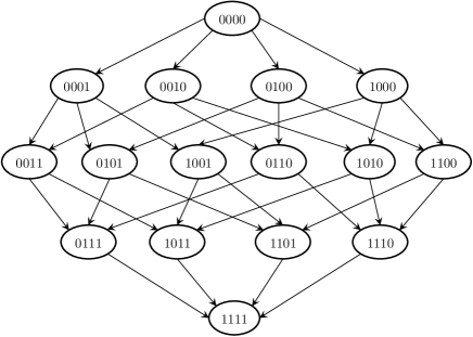
(c)

Figure 2: Selection of the representative sets for $F=4$ that achieve the capacity, Example 2. (a) Multisymbols for the $12$ inputs with minimal expected Hamming distance $1$. (b) Multisymbols for the $12$ inputs with minimal expected Hamming distance 0.75. (c) Graph representation of the process for selecting the multisymbols $\mathbf{x}_{s}(t)$. Both sets are constructed based on the same graph representation, only the selected paths in the graph for the corresponding multisymbols are different in the two sets.

The previous observations lead us to ask if there is a general strategy that produces the choice of the set of multisymbols for an arbitrary $F$ which has the maximal minimal expected Hamming distance? The answer is affirmative. Without giving a detailed proof, we will only note that this set is implicitly constructed in Appendix, Part I [1], where it is shown that it is always possible to choose the $L=\mathrm{lcm}\{\binom{F}{0},\binom{F}{1},\ldots,\binom{F}{F}\}$ paths in the direct graph. A careful examination of the argumentation in the proof reveals that a set of $L$ multisymbols with the required properties can be constructed by the procedure described in the proof.

Surprisingly, we have been able to find a set of multisimbols with minimal expected Hamming distance $0.75$ which performs better than the above set with minimal distance $1$, as presented in the simulation results in the next section. The set of multisymbols is presented on Fig. 2 b) and is obtained by using the same graph representation Fig. 2 c), only using different paths in the graph. We suspect that the reason for this behavior is that the minimal distance itself is not decisive for the performance, even if the conjecture that the expected Hamming distance is the relevant metric for the error-control coding holds. Probably, one has to look at both the distance spectrum and the trellis diagram in details, in order to make the right conclusion about the code performance. Nevertheless, the performance in both cases is superior to the naïve scheme, which makes the case for the relevance of the multisymbol framework in the design of practical error-control schemes.

III-B3 Choice of the multisymbols, Example 3

As a third example, we choose the $12$ multisymbols as shown in Fig. 3 a). We notice that, according to this choice, the multisymbols $t_{1}$ and $t_{2}$ are identical. Actually, besides $t_{1}=t_{2}$, we have also $t_{5}=t_{6}$ and $t_{10}=t_{11}$. We note that this choice does not violate the conditions for minimal multisymbols and satisfies the target distribution over $X$, thus it is capacity achieving.

$t$	$\{\mathbf{x}_{s}(t)\}$
$1$	$(0000,0001,0011,0111,1111)$
$2$	$(0000,0001,0011,0111,1111)$
$3$	$(0000,0001,0101,0111,1111)$
$4$	$(0000,0010,0110,1110,1111)$
$5$	$(0000,0010,1010,1011,1111)$
$6$	$(0000,0010,1010,1011,1111)$
$7$	$(0000,0100,0101,1101,1111)$
$8$	$(0000,0100,0110,1110,1111)$
$9$	$(0000,0100,1100,1101,1111)$
$10$	$(0000,1000,1001,1101,1111)$
$11$	$(0000,1000,1001,1101,1111)$
$12$	$(0000,1000,1100,1110,1111)$

(a)

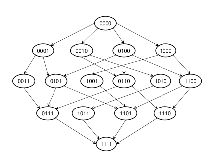
(b)

Figure 3: Selection of the representative sets for $F=4$, Example 3. The selection of the multisymbols yields non-uniform distribution of $\mathcal{T}$. (a) Multisymbols for the $12$ inputs (b) Graph representation of the process for selecting the multisymbols $\mathbf{x}_{s}(t)$.

At the first sight, this result seems counterintuitive and reveals the following problem: why we do not lose capacity even if we are not using the highest possible diversification at the input (in this case we assign the same multisymbol to two input symbols $t$)? We note that the cardinality of the input symbols is not $12$, but $9$. However, they are non-uniformly distributed — for example, $6$ have probability $\frac{1}{12}$ and $3$ have probability $\frac{1}{6}$. Until now, we have constrained ourselves to uniform distribution over the input symbols. However, it can be shown that if non–uniform distribution is used over ${\cal T}$, then capacity can be achieved even with $|{\cal T}|<L=\textrm{lcm}\left(\binom{F}{0},\binom{F}{1},\ldots,\binom{F}{F}\right)$. For this particular instance with $F=4$, it can be shown that in the above example the capacity can be achieved by a set $\mathcal{T}$ with cardinality $|{\cal T}|=8$. The probability distribution of the input symbols ${\cal T}$ is $P_{T}(t)=\frac{1}{6}$ for $t=1,2,3,4$ and $P_{T}(t)=\frac{1}{12}$ for $t=5,6,7,8$. In the following we specify only the nonzero members $\mathbf{P}$, the transition matrix for the channel $T-\mathbf{X}$. Note that the notation is slightly abused, with e. g. $P(0001|T=1,5)$ meaning $P(0001|T=1)$ or $P(0001|T=5)$): $P(0000|T=t)=P(1111|T=t)=\frac{1}{16}\quad\textrm{for any }t=1\ldots 8$; $P(0001|T=1,5)=P(0010|T=2,6)=P(0100|T=3,7)=P(1000|T=4,8)=\frac{4}{16}$ $P(0011|T=1)=P(0110|T=2)=P(1100|T=3)=P(1001|T=4)=\frac{6}{16}$; $P(0101|T=5,7)=P(1010|T=6,8)=\frac{6}{16}$, and $P(0111|T=1,5)=P(1110|T=2,6)=P(1101|T=3,7)=P(1011|T=4,8)=\frac{4}{16}$. The general case of $T-\mathbf{X}$ with non–uniform distribution on ${\cal T}$ and minimal required size $|{\cal T}|$ to achieve the capacity is outside of the scope for this paper and is a topic of ongoing work.

In the following section we present worked-out examples of trellis codes based on the multisymbol framework.

IV Code Design and Simulation Results

IV-A Code Design

The coding scheme we propose is designed as a concatenation of an outer error correcting code, an interleaver and an encoder, as given in Fig. 4 a). The outer error correcting code is a convolutional code with rate $1/2$, thus $2n$ binary symbols are generated from $n$ symbols. As already discussed, the inner code is trellis based, each branch in the trellis is associated with an input symbol (binary) and output symbol which is one of the $L$ multisymbols. We associate multisymbols with the transitions in the trellis such that the output symbols on the branches exiting from the same state should be maximally separated in terms of expected Hamming distance. The same is valid for the output symbols associated with the two branches that enter the same state. The trellis encoder codes incoming binary symbols into multisymbols which are then impaired by the channel. In this part we assume a binary erasure channel. However, we have in mind that the capacity results presented in Part I are valid for a wider class of channels, among others the binary symmetric channel and the $Z$ channel.

The symbol errors from a trellis code come in bursts since ending up in a wrong state implies more than one symbol error. To avoid bursts of errors, an interleaver is used. The interleaver is implemented as matrix with dimensions $\lambda\times\frac{2n}{\lambda}$ with $2n$ divisible by $\lambda$. In order to illustrate the coding scheme, we take once again the example with $F=4$. The trellis based coding scheme for $F=4$ defines a trellis with $12$ branches. One option is to consider a code with $4$ states and $3$ branches from each state or a code, which implies that the source information is originally encoded in ternary symbols. Another, more practical option is to have a trellis with $6$ states and $2$ branches from each state. The code construction uses the trellis code with $6$ states to avoid mapping from binary symbols to ternary symbols. This means that one binary symbol is transmitted for each multisymbol. The trellis design for the two sets of multisymbols introduced in Section III with respective minimal distance $0.5$ and $1$ is presented on Fig. 4. We recall that the first set was described by a directed graph where some of the multisymbols share common edges which could be avoided. The trellis is given in Fig. 4 b). The second set is chosen according to the criterion which maximizes the minimal expected Hamming distance. The trellis for the second set is illustrated in Fig. 4 c). In both cases, the multisymbols which are associated with the transitions in the trellis are chosen such that the output symbols on the branches exiting from the same state are maximally separated in terms of the expected Hamming distance. Similarly, in both cases, the distance between the output multisymbols is $2.5$ for all states. This is the maximal distance in the distance spectrum. The same is valid for the output symbols associated with the two branches that enter the same state.

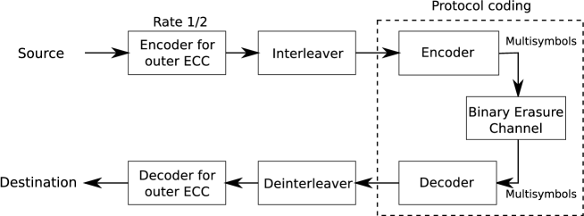
(a)

(b)

(c)

Figure 4: Code Design. a) Block diagram of the code. b) Trellis construction for the set of multisymbols of Example 1. (c) Trellis construction for the set of multisymbols of Example 2.

IV-B Simulation Results

The simulations have been performed with $\lambda=8$ and the results are averaged over 10000 iterations. The simulation is performed for packet lengths $N=\{2,6,14,30,62\}$. These packet lengths are chosen such that $N+2$ (two tail bits are added by the outer convolutional code) is divisible by $\lambda=8$.

First, we compare the performance of the coding scheme inspired by the multisymbol framework and the naïve coding scheme, which does not account for the specifics of the secondary channel. The simulation results for the packet error rate (PER) for different erasure probability are shown in Fig. 5. This result present a clear evidence that the information-theoretic analysis carries a practical significance for the secondary communications channels.

We also perform simulations for the two different choices of the sets of multisymbols, with minimal expected Hamming distance $0.5$ and $1$ respectively, as presented in Section III. As already commented, although the choice of the set with minimal distance $1$ performs better than the set with minimal distance $0.5$ ( Fig. 6 a)), we were able to find another set with minimal distance $0.75$ which outperforms both sets (Fig. 6 a)). This result indicates that besides the minimal expected Hamming distance is not the only criterion which decides on the code performance, but there are also factors, notably the distance spectrum and the choice of the trellis transitions.

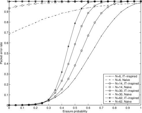
Figure 5: Performance comparison between the naïve coding scheme and the scheme motivated from the multiuser framework

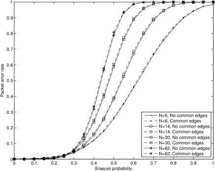
(a)

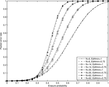
(b)

Figure 6: Performance of the error-correcting coding schemes. (a) Comparison between two sets with minimal distance $0.5$ and $1$ respectively. (b) Comparison between two sets with minimal distance $0.75$ and $1$ respectively.

V Discussion

V-A Some Features of the Secondary Channel

In Part I [1] we have described a generic application of this type of protocol coding and the associated secondary channel: communication with newly introduced devices, with limited functionality, in an area that is larger than the original coverage area. Several distinctive features can be noted for this type of secondary communication. First, for delay-constrained systems, the secondary data rate is relatively low, so it is hard to argue that this method brings a significant rate advantage. Second, the secondary rate depends on the current load (traffic, number of users) in the primary system. For example, in a cellular system where protocol coding is done by encoding information in the way the users are allocated to different channels, the best secondary rate on is obtained when each channel can be allocated to a different user, since this maximizes the number of possible rearrangements. Third, the new secondary devices have a limited implementation of the primary protocol stack, which brings opportunity for a low–complexity, low–power reception on the secondary channel. In the extreme case, protocol coding reckons only with two transmission states: packet transmitted and idle slot, as with the $Z-$channel model, which would require the secondary device to use only power detection.

Header compression [3] may appear as a competitor as it works in a somewhat opposite way: tries to compress the overhead whenever the actual communication scenario allows it. However, this is not always cancelling the opportunity for secondary communication, and vice versa: for example, the MAC–layer identifiers may be compressed, but in the end all the users have to be differentiated and the secondary channel arises from reordering those identifiers. An interesting dividend is that the secondary capacity can be used to assess the performance margin of a certain primary protocol/system. Intuitively, if in a given scenario the secondary capacity is non–zero, then the operation of the primary system is not optimal.

The secondary channel, as defined here, can have several different application. A generic application of the secondary communication is sending of additional control data. The first usage of such a control data can be as expanded “future use” bits: in many standardized protocols there are unspecified, free bits for future use and protocol coding practically unleashes “hidden” future use bits in the protocol, which may become indispensable during the evolution of the system.

Another usage can be signaling for efficient spectrum sharing. The main concern in cognitive radio is the interference that the cognitive (secondary) users are causing to the incumbent (primary) user. Hence, a secondary user should sense if the spectrum resource is available for communication. Spectrum sensing is facilitated by a Cognitive Pilot Channel (CPC) [4], which conveys the necessary information to the terminals about the status of radio spectrum. Protocol coding inherently introduces a possibility to define an in–band CPC. For example, assume that, besides the module that can decode the secondary channel, the secondary devices have an additional cognitive radio interface to communicate with each other. Then the primary BS can dynamically send information about the available resources for cognitive radio. For example, if the primary system is a digital TV broadcaster, then secondary channel can be defined by reordering of the TV packets, which empowers the TV broadcast tower to dynamically control the spectrum usage. To the best of our knowledge, such a possibility to turn the TV broadcasters from victims into spectrum controllers has not been observed before.

In the emerging machine–to–machine (M2M) communication [5], cellular networks embrace a large number of low–cost, low–power devices, that have different traffic/behavior from the usual cellular users. Such a device device is mostly in a low–power “sleep” mode. We conjecture that, due to the simple codebooks used to send the primary control information, it can be decoded with a low power. A sleeping device may be tuned receive on the secondary channel and, upon receiving a downlink trigger from the BS, it can wake up another radio interface to send information. Thus, protocol coding offers an opportunity to introduce universal wake–up beacons.

V-B Protocol Coding in WiMAX: A Brief Case Study

We now illustrate the application of protocol coding with reordering of user resources to the WiMAX system. In WiMAX [6], the downlink and uplink control information is transmitted at the beginning of each frame, which includes preamble, frame control header (FCH) and MAP message. The MAP message indicates the resource allocation for downlink and uplink data and control signal transmission. The Base Station (BS) translates the QoS requirements of the Subscriber Stations (SSs) into the appropriate number of allocated slots. The BS informs about the scheduling to all SSs by using the DL_MAP (Downlink Medium Access Protocol) and UL_MAP (Uplink Medium Access Protocol) messages in the beginning of each frame [7].

Protocol coding is implemented by reordering the slots allocated in a frame. The secondary users for which this information is intended have only to read the broadcast DL_MAP and UL_MAP messages. For example, when the number of slots reserved for each of the SSs is 6,9,2,10,7,6,10,15,15,20 respectively, $289$ secondary bits can be sent by reordering of the resources. Assuming a frame duration of $5ms$, this translates to we can have $\approx 58$ [kbps] of additional information, which is in the frame headers that are robustly protected [8]. In order to get an idea about the the distance where the MAP message is “detectable”, compared to the information data, we resort to the propagation model in [8], with the total path loss is given by $L=126,2+36\log d$ [dB], where $d$ is in kilometers. The MAP is protected with $6-$times repetition coding, while and BPSK is used for both MAP message and data, which results in distance $d^{\prime}\approx 1.65\>d$ where the header is detectable compared to the distance $d$ for the user data.

V-C Further Considerations

We used a simplified model, in which the set of packets sent in a given frame is independent from the other frames. In practice this is rarely satisfied, since buffering at the primary scheduler and/or packet retransmission due to errors creates dependencies between consecutive frames. In such a case, Shannon’s result is not directly applicable and instead we need to use a more general model in which the sequence of frame states is not memoryless (see Section 6 in [9]).

Another aspect is the freedom of in reordering user resources. For example, if in the case of WiMAX the scheduler puts each user on a channel where she can achieve a high data rate, then the freedom to permute users across channels becomes restricted. It is incorrect to say that protocol coding is not applicable once such restrictions are put by the primary system, but it should rather be observed that the secondary capacity is decreased. This reiterates the observation that protocol coding can be used as a measure of how optimally given primary system operates.

We have mainly discussed the case of the combinatorial model with two possible packet values $0,1$. In general, the number $m$ of possible packets in a frame can be $1\leq m\leq F$, where the special case $m=F$ corresponds to the permutation model. As coding strategies, it is relevant to consider the permutation codes used in power line communication(PLC) [10]. The main idea is to send information by using $M-$ary Frequency Shift Keying (FSK). There are $M$ available orthogonal frequencies and transmission is done by creating a time sequence by which the frequencies are activated. This corresponds to a permutation without repetitions of size $M$ and the correspondent codes can be used as coding strategies in our permutation model. The main idea is to define a Hamming distance between two permutations and only permutations that are sufficiently distant are eligible for transmission in order to minimize the probability of error. A more general case is the one where the transmission symbol (frame) has $F>M$ frequencies and the $i-$th frequency appears $f_{i}$ times, such that $\sum_{i=1}^{M}f_{i}=F$. The codes used in that case are termed constant composition codes [11]. However, the main design constraint for permutation codes in PLC scenarios is not to create a disturbance to the electric power. This implies that there is a freedom to choose the set $\{f_{i}\}$ as long as the power constraint is satisfied; on the contrary, in our model the secondary transmitter must reckon with the set $\{f_{i}\}$ provided by the primary communication system. Nevertheless, the code design from frequency permutation arrays in PLC may be used to select the components of the multisymbols for protocol coding.

VI Conclusion and Future Work

We have investigated practical strategies for protocol coding via combinatorial ordering of the user resources (packets, channels) in the primary system. By using the specific structure of our model, we have used the alternative framework that helps to compute the capacity in the development of coding strategies that are approaching the capacity. The developed coding strategies are superior to the naïve strategy which does not account for the specifics of the secondary communication channels. The coding design thus gives practical relevance to the framework developed for capacity characterization of secondary channels and paves the road for practical implementation. Besides the construction of the coding schemes, we also presented some additional features of protocol coding and pointed out possible applications of the concept in existing wireless systems.

A question for future work is how to compute the capacity and which coding strategies to use when the scheduling process in the primary system is generalized (buffering, retransmission, etc.). Another direction is to compute the capacity under error models different from the described, such as channels with deletions/insertions. In practice, a secondary channel can be defined over virtually any existing wireless system and therefore it is of interest to find the coding strategies that are suited to the actual protocol specification in a certain primary system.

References

- [1] P. Popovski and Z. Utkovski, “Protocol Coding through Reordering of User Resources, Part I: Capacity Results,” submitted to IEEE Trans. Communications, 2012.
- [2] P. Popovski and O. Simeone, “Protocol Coding for Two-Way Communications with Half-Duplex Constraints,” in IEEE GLOBECOM, Miami, FL, USA, Dec. 2010.
- [3] H. Hannu, L.-E. Jonsson, R. Hakenberg, T. Koren, K. Le, Z. Liu, A. Martensson, A. Miyazaki, K. Svanbro, T. Wiebke, T. Yoshimura, and H. Zheng, “RObust header compression (ROHC): Framework and four profiles: RTP, UDP, ESP, and uncompressed,” in RFC 3095, Jul. 2001.
- [4] J. Perez-Romero, O. Sallent, R. Agusti, and L. Giupponi, “A Novel On-demand Cognitive Pilot Channel enabling Dynamic Spectrum Allocation,” in Proc. IEEE DySPAN, Dublin, Ireland, Apr. 2007.
- [5] S.-Y. Lien, K.-C. Chen, and Y. Lin, “Toward Ubiquitous Massive Accesses in 3GPP Machine-to-Machine Communications,” IEEE Communications Magazine, vol. 49, no. 4, pp. 66–74, Apr. 2011.
- [6] J. G. Andrews, A. Ghosh, and R. Muhamed, Fundamentals of WiMAX. Prentice-Hall, 2007.
- [7] A. Sayenko, O. Alanen, J. Karhula, and T. Hämäläinen, “Wimax Overview and System Performance,” in Proceedings of the 9th ACM MSWiM, Torremolinos, Spain, Oct. 2006.
- [8] F. Wang, A. Ghosh, C. Sankaran, and P. Fleming, “Wimax Overview and System Performance,” in Proc. IEEE VTC Fall, Sep. 2006.
- [9] G. Keshet, Y. Steinberg, and N. Merhav, Channel Coding in the Presence of Side Information, ser. Foundations and Trends in Communications and Information Theory, 2007, vol. 4, no. 6.
- [10] A. J. H. Vinck, “Coded Modulation for Power Line Communications,” AEÜ Journal, pp. 45–49, Jan. 2000.
- [11] W. Chu, C. J. Colbourn, and P. Dukes, “Constructions for Permutation Codes in Powerline Communications,” Designs, Codes and Cryptography, Kluwer Academic Publishers, vol. 32, pp. 51–64, 2004.