Neutrinos and cosmic rays

Abstract

In this paper we review the status of the search for high-energy neutrinos from outside the solar system and discuss the implications for the origin and propagation of cosmic rays. Connections between neutrinos and gamma-rays are also discussed.

1 Introduction

Observation of high-energy neutrinos of astrophysical origin would open a new window on origin of cosmic rays. Neutrinos are expected at some level in association with cosmic rays, both from interactions of accelerated protons and nuclei in or near their sources and from interactions of the cosmic rays during propagation in space. Production of high-energy neutrinos requires interaction of hadrons to make mesons which then decay to neutrinos. Observation of neutrinos from gamma-ray sources would therefore indicate a hadronic rather than electromagnetic origin for the photons. Examples of possible sources are galactic supernova remnants and extragalactic objects such as gamma-ray bursts (GRB) and active galactic nuclei (AGN).

In addition, wherever gamma-rays are produced by interactions of cosmic rays during their propagation, neutrinos will also be produced. Examples of the latter are neutrinos related to the diffuse gamma-ray emission from the disk of the Milky Way [1] and cosmogenic neutrinos produced when cosmic rays of ultra-high energy (UHECR) interact with the cosmic background radiation (CMB) [2]. Both processes can be calculated in a straightforward way. For the Galaxy, the physics is pion production in interactions of cosmic rays with gas in the interstellar medium, and the neutrino flux follows directly from the observed diffuse gamma-radiation from the same source. The calculation of photo-pion production by protons in the cosmic microwave background (CMB) also follows from well-known physics, but in this case the level of neutrino production is highly uncertain because the ultra-high energy cosmic ray (UHECR) spectrum is unknown. Whether there are sufficient protons above the threshold of $3\times 10^{19}$ eV is one of the main unanswered questions of neutrino astronomy.

The discovery of neutrino oscillations [3] has important implications for neutrino astronomy. One expects only muon and electron neutrinos to be produced both in interactions with gas and in photo-pion production. However, the effect of oscillations on an astronomical baseline is that the initial flavor ratio evolves toward comparable numbers of all flavors for the observer. For example, for an initial flavor ratio of $\nu_{e}:\nu_{\mu}:\nu_{\tau}\,=\,1:2:0$ the ratio at Earth would be $1:1:1$ [4]. Since tau neutrinos are essentially absent above $100$ GeV in the atmospheric neutrino background, identification of a $\nu_{\tau}$ would be strong evidence for astrophysical origin. For this reason, the ability to distinguish neutrino flavors is important.

2 Status of searches for neutrino sources

The biggest signal is expected in the muon neutrino channel. Because of the long range of high energy muons, interactions of $\nu_{\mu}$ outside the detector can produce muons that reach and pass through the detector. For an instrumented volume even as large as 10 km³, the external $\nu_{\mu}$ events are more numerous than interactions inside the instrumented volume. The most sensitive searches use the Earth as a filter against the downward background of atmospheric muons by requiring the muon track to be from below the horizon.

The most basic approach to neutrino astronomy is to look for an excess of events from a particular direction in the sky. AMANDA, Baikal, Antares and IceCube all make sky maps. The search can be binned or unbinned [5]. After accounting for the effective number of trials, no significant excess has been seen in any detector. A related approach is to look for an excess of events from a list of objects selected because they are likely neutrino sources. The source list for IceCube [6], for example, includes 13 galactic supernova remnants (SNR), and 30 extra-galactic objects, mostly AGN. With its instrumented km³ volume, IceCube is by far the most sensitive detector at present. Published limits from IceCube during construction with 40 strings installed (IC-40) on specific point sources of neutrinos in the Northern sky are less than $10^{-11}$cm^-2s^-1TeV^-1. With the full IceCube the sensitivity is now approaching $10^{-12}$cm^-2s^-1TeV^-1, at which level TeV gamma-rays are seen from some blazars such as Mrk 401 [7].

A related approach is to look for neutrinos correlated in time, either with each other or with a gamma-ray event [8]. The strongest limit from IceCube in terms of constraining models that relate cosmic-ray origin with production of neutrinos is the absence of neutrinos in coincidence with GRB. Recently data sets from two years of IceCube while the detector was still under construction (IC-40 and IC-59) have been combined to obtain a significant limit [9] on models [10] in which GRBs are the main source of extragalactic cosmic rays. In total 215 GRBs reported by the GRB Coordinated Network between April 5, 2008 and May 31, 2010 in the Northern sky were included in the search. No neutrino was found during the intervals of observed gamma-ray emission.

To set limits on the model [10], the expected neutrino spectrum was calculated for each burst based on parameters derived [11] from features in the spectrum of the GRB. In particular, a break in the observed photon spectrum marks the onset of photo-pion production by accelerated protons interacting with intense radiation fields in the GRB jet. The neutrinos come from the decay of charged pions. Given a predicted neutrino spectrum, the expected number of events was calculated for each burst. The normalization of the calculation is provided by the assumptions that a fraction of the accelerated protons escape and provide the ultra-high energy cosmic rays. In the simplest case, the UHECR are injected as neutrons from the same photo-production processes in which the neutrinos are produced [12]. With this normalization, 8 neutrinos are expected in 215 GRBs and none is observed.

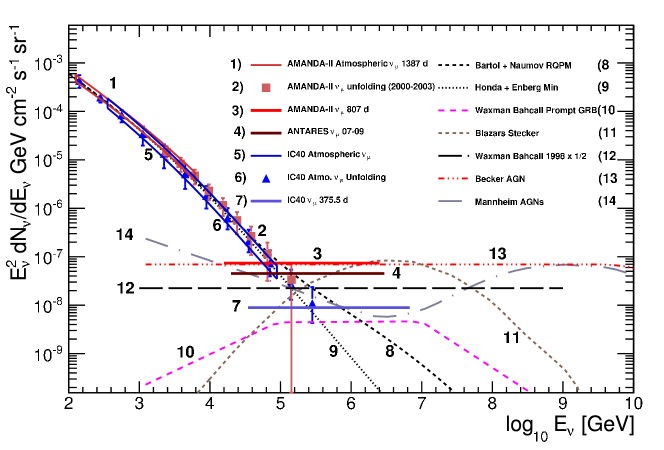
Figure 1: Horizontal lines show limits on an $E^{-2}$ spectrum of astrophysical muon neutrinos from AMANDA-II [13], Antares [14] and IceCube [15]. The plot is from Ref. [15] where full references are given. The limits are shown along with measurements of the flux of atmospheric muon neutrinos and anti-neutrinos.

3 Neutrinos from the whole sky

It is important also to search for an excess of astrophysical neutrinos from the whole sky at high energy above the steeply falling background of atmospheric neutrinos. The Universe is transparent to neutrinos, so the flux of neutrinos from sources up to the Hubble radius may be large [30]. A toy model is helpful to illustrate this point. Assume a distribution of identical sources of neutrino luminosity $L_{\nu}$ (s^-1TeV^-1) with a typical separation of order $d=10$ Mpc. The flux from a nearby source is $L_{\nu}/(4\pi d^{2})$ (s^-1TeV^-1cm^-2). Integrating over the whole sky with a cutoff at the Hubble distance $D_{H}$ the flux from the whole sky is

$$\phi\,\approx\,\int_{0}^{D_{H}}\,{\rho\,L_{\nu}\,r^{2}\over 4\pi r^{2}}{\rm d}\Omega{\rm d}r,$$ (1)

where $\rho\sim 1/d^{3}$ is the density of sources. In this case the ratio of the total flux of neutrinos from all directions to the flux from a nearby source is $\sim 4\pi\,D_{H}\,/\,d\,\sim\,4000$ for $d=10$ Mpc. Later we will cite examples of calculations for specific models of AGNs and GRBs, which take account properly of red shift for distant sources. In some cases the predicted diffuse fluxes are sufficiently high to constrain the models more than the point source searches. Before discussing the models, we first summarize the current status of the limits on diffuse fluxes of high energy neutrinos.

The limit from IC-40, shown as the solid (blue) line #7 in Fig. 1, is from an analysis of approximately 14,000 upward neutrino-induced muons in IC-40 [15]. This analysis proceeds by assuming a flux of neutrinos with three components: conventional atmospheric neutrinos from decay of kaons and pions; prompt neutrinos; and a hard spectrum of astrophysical neutrinos assumed to have an $E^{-2}$ differential spectrum. Free parameters in fitting the data are the normalization of the prompt and astrophysical neutrinos. The normalization and slope of the atmospheric neutrinos are also allowed to vary within a limited range. The result is consistent with conventional atmospheric neutrinos, with no need for a contribution from prompt neutrinos and no evidence of a hard spectrum of astrophysical neutrinos. A limitation of the analysis is that the atmospheric neutrino background is represented by a simple power law extrapolation of the calculation of Ref. [19] beyond $10$ TeV, and it averages over all angles below the horizon.

Also shown in Fig. 1 are several measurements of the flux of atmospheric neutrinos. The fit for atmospheric neutrinos from the IC-40 analysis that gives the diffuse limit is shown as a slightly curved band extending from 0.33 to 84 TeV. The reason that the diffuse limit applies at much higher energy (39TeV to 7 PeV) is that it assumes a hard, $E^{-2}$ differential energy spectrum for the neutrinos, in contrast to the steep ($\sim E^{-3.7}$) atmospheric spectrum. The other experimental results on the high-energy flux of atmospheric $\nu_{\mu}+\bar{\nu}_{\mu}$ in Fig. 1 are from AMANDA [16, 17] and IceCube-40 [18]. All the atmospheric neutrino spectra shown here are averaged over angle. The unfolding analysis of Ref. [18] extends to $E_{\nu}\approx 400$ TeV. The atmospheric fluxes shown are averaged over the upward hemisphere. At high energy atmospheric neutrinos from decay of charged pions and kaons have a significant angular dependence (the “secant theta” effect) with the intensity increasing toward the horizon. This angular dependence will be important in distinguishing atmospheric background from astrophysical signal in future analyses.

At the current level of sensitivity in the search for high-energy astrophysical neutrinos, the energy range where the atmospheric neutrino background becomes important is at 100 TeV and above, as illustrated by the crossover of the limits and the atmospheric fluxes in the Fig. 1. This energy is well beyond the range of detailed Monte Carlo calculations [19, 20], which extend only to $10$ TeV. In addition, this is the energy range where prompt neutrinos from decay of charm and heavier flavors may become important, but the expected level of this contribution is uncertain. The spectrum of prompt neutrinos is harder by one power than the spectrum of conventional atmospheric neutrinos in this energy range, and its angular distribution is isotropic. These features mimic a diffuse astrophysical flux to some extent. A possible strategy is to determine the level of prompt lepton production with atmospheric muons which would remove the ambiguity from this contribution to the background of atmospheric neutrinos. Calculations that extend the atmospheric neutrino flux up to the PeV range will also need to account for the primary composition in the knee region keeping in mind that what is relevant is the spectrum of nucleons as a function of energy per nucleon.

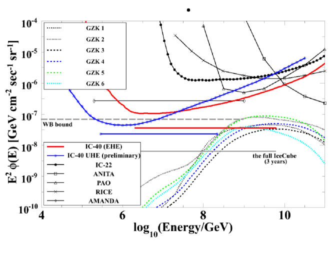
Figure 2: Collection of limits on cosmogenic and ultra-high energy neutrinos of all flavors. The plot is based on Ref. [21] where full references are given. The extra curve included here, labeled IC-40 UHE (preliminary) is from Ref. [22].

Figure 2 summarizes searches for neutrinos of higher energy, including the region relevant for cosmogenic neutrinos. Limits on the high energy side from Auger [23] and ANITA [24, 25] are shown as well as the results at lower energy from IC-40. In the IC-40 analysis shown here [21], the strategy is to look for extremely energetic events where the atmospheric neutrino background should not be important. The greatest sensitivity in this energy range is to events near the horizon because vertically upward muons are absorbed by the Earth. The contribution of $\nu_{\tau}$ is particularly important. For the Auger analysis, $\tau$ leptons produced by charged current interactions of $\nu_{\tau}$ skimming the earth are expected to give the major signal as the $\tau$ leptons decay over the array [26]. Around $10^{6}$ GeV in IceCube an important contribution to an astrophysical signal would come from $\nu_{\tau}$ regeneration in the Earth [27]. Simulations show that a significant fraction of the events generated by cosmogenic neutrinos would appear as cascade-like events generated by $\nu_{e}$ and $\nu_{\tau}$. The appearance of $\nu_{\tau}$ depends on energy. For $E\approx 10^{6}$ GeV a charged current interaction inside IceCube would give a “double bang” event [4] with two separated cascades, one when the $\nu_{\tau}$ interacts and the other when the $\tau$ decays. At lower energy there would be a single, perhaps elongated, cascade and at higher energy a cascade plus the track of a $\tau$-lepton either entering or leaving the instrumented volume.

The horizontal dashed lines in Figs. 1 and in Fig. 2 show a benchmark intensity, the Waxman-Bahcall limit. Current IceCube limits are below the original Waxman-Bahcall limit [28]. We discuss the implications of this fact later in the section on extragalactic sources.

4 Production of astrophysical neutrinos

Since we have not yet detected neutrinos arriving to us from astrophysical sources we have to use the existing gamma ray data to identify sources that are likely to produce neutrinos. There are two different ways to produce neutrinos in astrophysical sources. One is from interactions of accelerated protons and nuclei on matter. All kinds of mesons are produced and the charged mesons decay to muons and neutrinos while the neutral mesons decay mostly into gamma rays. It is easy to do a rough estimate of the relation of the neutrino and gamma ray fluxes from pion decay. If the gamma ray flux from $\pi^{0}$ decay is $\phi_{\gamma}\;=\;C\times E_{\gamma}^{-\alpha}$ the corresponding muon neutrino and antineutrino spectrum from $\pi^{\pm}$ decay is $\phi_{\nu}\;=\;C\times(1-r_{\pi})^{\alpha-1}\times E_{\nu}^{-\alpha}$, where $r_{\pi}$ = $(m_{\mu}/m_{\pi})^{2}$. Since in astrophysical environments muons usually also decay, this flux is doubled and becomes roughly equal to the photon flux. It is also straightforward to take into account the muons and neutrinos from decay of kaons. The exact calculations are algebraically complicated because of polarization effects in muon decay [30]. For a power-law distribution of protons with differential index $\alpha$ the ratio of $\nu_{\mu}+\bar{\nu}_{\mu}$ to photons is $1.0$ for $\alpha=2.0$ and $0.7$ for $\alpha=2.7$. We will start with the assumption that production via proton interactions in gas contributes the most to the neutrino production in many galactic sources (like supernova remnants and molecular clouds) where the matter density provides enough target for nuclear interactions.

Neutrinos are also produced in interactions of protons with ambient photons, $p\gamma\rightarrow N\pi$. Possible photon backgrounds are those in jets of AGN and gamma ray bursts (GRB) as well as the CMB. The proton threshold energy for production of pions is $E_{p}^{thr}\;=\;{{m_{\pi}}\over{4\epsilon}}(2m_{p}+m_{\pi})$, where $\epsilon$ is the energy of the photon in the lab system. In the CMB ($\langle\epsilon\rangle$ = 6.3$\times$10^-4 eV) the proton threshold energy, calculated with the exact CMB spectrum is 3$\times$10¹⁹ eV. It is more difficult to estimate the threshold energy and the secondary particle spectra in AGN or GRB jets where the photon background spectra usually have non-thermal, typically broken power-law spectra. One can simplify the estimate by assuming that all pion photoproduction goes through the $\Delta^{+}$, i.e. $p+\gamma\rightarrow\Delta^{+}\rightarrow p\pi^{0}(np^{+})$, which is a reasonable approximation especially in the case of a steep proton spectrum interacting with thermal distribution of photons where most of the production occurs near the kinematic threshold. In the $\Delta^{+}$ approximation the production of neutral pions is twice that of $\pi^{+}$. The $\gamma$-rays from $\pi^{0}\rightarrow 2\gamma$ decay would have higher energy than the neutrinos from the $\pi^{+}\rightarrow\nu_{\mu}+\mu\rightarrow\bar{\nu}_{\mu}+\nu_{e}$ decay chain. In general, the ratio of the final energies of the $\gamma$-rays to neutrinos is greater than one, but when production above the $\Delta$ resonance region is important, the ratio of charged to neutral pions is increased.

An essential complication from the point of view of neutrino astronomy is that gamma-rays can also be produced in purely electromagnetic processes whenever accelerated electrons are present in the sources. Synchrotron radiation is important at low energy and inverse Compton scattering at high energy, as well as bremsstrahlung when there is sufficient gas present to scatter the electrons.

Figure 3 shows the location of galactic and extragalactic sources of TeV gamma rays from the TeVCat catalog [31]. In the following sections we discuss examples of these objects as potential neutrino sources.

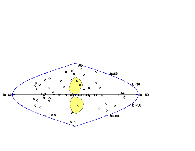
Figure 3: Extragalactic (circles) and galactic (pluses) TeV gamma ray sources from the TeVCat catalog. A large number of unidentified sources, some of which have distance estimates, are not plotted. The two shaded regions indicate the Fermi bubbles. There is also diffuse emission from the galactic plane, which is not shown here.

5 Galactic neutrinos

5.1 Neutrinos produced during propagation

To the extent that the diffuse gamma radiation from the plane of the Milky Way is due to interactions of cosmic rays with gas in the interstellar medium through the $\pi^{0}$ channel, there will be a corresponding level of diffuse neutrinos [1]. For power law spectra there is a simple proportionality described in the previous section whereby

$${{\rm d}N_{\nu_{\mu}+\bar{\nu}_{\mu}}\over{\rm d}E_{\nu}}\,\sim\,{{\rm d}N_{\gamma}\over{\rm d}E_{\gamma}}$$ (2)

The newer analyses of the TeV $\gamma$-ray flux show that at such high energy the production of $\gamma$-rays is dominated by inverse Compton scattering of accelerated electrons

Recently the Fermi LAT collaboration has reported diffuse regions of gamma emission extending to large distances both above and below the galactic center as shown in Fig. 3. There are competing models of the gamma rays, one of which involves second order Fermi acceleration of electrons by magnetic turbulence [32] and the other which postulates a steady, long term production of gamma rays by collisions of trapped cosmic rays with diffuse gas [33]. In the latter case, there would be a corresponding level of neutrino production given by Eq. 2. If the energy spectrum of protons contained in the Fermi bubbles is flatter than E^-2.3 they would produce neutrino fluxes detectable in the Northern hemisphere [34]. The detection from the Southern hemisphere will be more difficult as a smaller portion of the bubbles is visible in upward going neutrinos.

The Fermi/LAT collaboration studied the fraction of $\gamma$-rays that are generated by protons during propagation by scattering on the galactic matter. They correlated this fraction of the gamma ray flux with the column density in a part of our Galaxy and established an emissivity of 0.66$\times$10^-26 photons.s^-1sr^-1H-atom^-1 above 300 MeV [35]. Scaled to $\gamma$-rays of energy above 1 TeV with an E^-2.7 cosmic ray spectrum this gives an emissivity of 6.8$\times$10^-11 photons.s^-1sr^-1 for column density of 10²² hydrogen atoms/cm^-2, very close to the old estimate [36] of 6$\times$10^-11. Since Ref. [36] has a model of the column density of the Galaxy we can now estimate the flux of neutrinos from the galactic plane taking account of the detector location.

IceCube can not see the inner galaxy in upgoing neutrinos. The closest it can get to it is $l$ = 31.8^o. We can define an area in longitude from 31.8^o to 90^o and latitude of 5^o around the galactic plane that has an average column density of 1.8$\times$10²² H-atoms/cm^-2. The angular area of that part of the galactic plane is 0.176 sr. The $\gamma$-ray flux above 1 TeV in this solid angle should be 1.9$\times$10^-11 cm^-2s^-1 and the neutrino muon neutrino and antineutrino flux should be 0.7 of that for ($\alpha$ = 2.7, i.e. 1.3$\times$10^-11 cm^-2s^-1).

Northern detectors, such as ANTARES or KM3Net, are able to observe the region of the inner galaxy. Cutting a similar region from $l$ = -90^o to 90^o we obtain an area of 0.546 sr with an average column density of 2.1$\times$10²² Hydrogen atoms/cm^-2. The neutrino flux from that solid angle should be 4.8$\times$10^-11 cm^-2s^-1.

To estimate the event rate we need to calculate the neutrino effective area of the detectors, which is defined so that, given a differential neutrino flux $\phi_{\nu}(E_{\nu})$, the event rate is

$${\cal R}=\int\,A_{\rm eff}(E_{\nu})\times\phi_{\nu}(E_{\nu})\,{\rm d}E_{\nu}.$$ (3)

The effective area depends on neutrino flavor and accounts for the detector response as well as the physics of the neutrino propagation and interaction. As an illustration here we consider $\nu_{\mu}+\bar{\nu}_{\mu}$ and an idealized detector that counts all muons above 100 GeV. In this case

$$A_{\rm eff}(E_{\nu})\,=\,P_{\nu}(E_{\mu})\times\exp[-\sigma_{\nu}(E_{\nu})N_{A}X(\theta)],$$ (4)

where $X(\theta)$ is the chord of the Earth at $\theta$ in g/cm², $N_{A}$ is the number of nucleons per gram and

$$P_{\nu}(E_{\mu})\,=\,N_{A}\,\int\,{\rm d}E_{\mu}{{\rm d}\sigma_{\nu}\over dE_{\mu}}(E_{\mu},E_{\nu})\,R_{\mu}(E_{\mu})$$ (5)

is the probability that a neutrino on a trajectory toward the detector produced a muon with enough energy to be detected and reconstructed. The muon range is $R_{\mu}$. The $A_{\rm eff}$ we use is 0.5, 1.0, 55 m² at 1, 10 and 100 TeV respectively for an ideal detector with a projected physical area of one square kilometer. Assuming the diffuse galactic spectrum continues with a differential spectrum of $-2.7$ to $E\gg 10$ TeV, the total flux from the region of the galactic plane visible to IceCube as estimated in the previous paragraph is $3\times 10^{-7}$ s^-1 or ten events per year. The flux is larger at Antares where the field of view includes the central region of the galaxy, but the projected area of the detector is much smaller than IceCube. Assuming it is $\leq 0.03$ km² there would be of order one event per year from this source in Antares. Ninety per cent of the integral comes from $E_{\nu}<10$ TeV.

5.2 Neutrinos from galactic cosmic-ray accelerators

Most of the galactic gamma ray sources shown in Fig. 3 (23 of 52) are pulsar wind nebulae similar to the first detected TeV source, the Crab nebula. The $\gamma$-ray production in the Crab nebula has been modelled many times and the successful models are all purely electromagnetic. Because of that we do not expect neutrino fluxes from such objects. There are also eleven supernova remnants (SNR) with identified shell like morphology and seven sources identified as SNR/Molecular Clouds. All these sources are SNR with close by dense molecular clouds. It is not always obvious if the gamma ray production is in a part of the supernova remnant or only in the molecular cloud.

The modeling of the gamma ray emission in supernova remnants started in Ref. [37]. It is based on the belief that the cosmic ray energy spectrum at the source is flatter than what we observe at the Earth. As an example the calculation was applied to the Tycho (1572) shell like supernova remnant which is likely to accelerate cosmic rays. Input parameters were the average SNR kinetic energy of 4.5$\times$10⁵⁰ ergs and the estimated matter density of 0.7 cm^-3 around the remnant. If 20% of all accelerated cosmic rays interact around the supernova the expected $\gamma$-ray flux above 1 TeV was estimated to be 1.2$\times$10^-12 (E_γ/TeV)^-1.1 cm^-2s^-1. The Tycho supernova was detected much later. Its gamma ray flux has indeed a flat spectral index $\alpha$ = 1.95$\pm$0.5$\pm$0.3 but much smaller flux at about 1% that of the Crab nebula. (1 Crab unit [38] corresponds to integral flux of 1.75$\times$10^-11 cm^-2s^-1 above 1 TeV.) It is obvious that it either accelerates fewer cosmic rays or contains them for a shorter time in the vicinity of the remnant. Defining a neutrino flux similar to such gamma ray flux requires much bigger neutrino telescopes than we have.

The HESS gamma ray collaboration published an analysis of their observation of the galactic center ridge [39] that partially explains why we have not seen as many $\gamma$-rays from supernova remnants as were initially predicted. The HESS group determined that the $\gamma$-ray emission from that part of the sky coincides with the positions of three molecular clouds with matter density of hundreds cm^-3. The total mass in these clouds is 2-4$\times$10⁷M_⊙. The observed $\gamma$-ray spectrum spectral index $\alpha$ = 2.3 is much flatter than the 2.7 spectrum we observe at Earth. The suggestion from this analysis is that we should look more at huge molecular clouds in the vicinity of supernova remnants rather than at the supernova remnants themselves.

In Ref. [40], the observed gamma-ray spectra from Egret [41] of two supernova remnants associated with molecular clouds were modeled in detail by considering the contributions from bremsstrahlung and inverse Compton up-scattering by electrons as well as photons from decay of neutral pions. The SNR $\gamma$-Cygni, at a declination of +40^o would give upward muons in IceCube. It has recently been detected in TeV photons by VERITAS [42]. Here we use the fit corresponding to Fig. 5 of Ref. [40], which assumed that $\gamma$-Cygni contains a single $\gamma$-ray source, to estimate the corresponding neutrino flux. Although the model fit is not dominated by $\pi^{0}$ photons the fit predicts a flux of $2.5\times 10^{-12}$cm^-2s^-1 at 1 TeV with a cutoff above 10 TeV from this source. The corresponding event rate, which is dominated by neutrinos in the range 0.3 to 3 TeV, is $3\times 10^{-8}$cm^-2s^-1, or one event per year, in IceCube.

6 Neutrinos of extragalactic origin

An estimate of the maximum neutrino flux from extragalactic sources was made by Waxman & Bahcall [28]. High energy neutrinos come from interactions of higher energy nucleons. Therefore any source of high-energy neutrinos is a potential source of cosmic rays. If the sources of the extra-galactic cosmic rays are transparent to nucleons so that they can inject cosmic rays into intergalactic space, then there is an implied limit on the associated flux of neutrinos from the condition that the sources not produce more cosmic rays than observed. In models in which protons are contained in the sources by the magnetic fields essential to their acceleration, the limit is related to an estimate of the expected neutrino flux [29]. Inside the accelerator, protons interact with photon backgrounds to photoproduce pions. Secondary protons from $p+\gamma\rightarrow p+\pi^{0}$ may be trapped and reaccelerated in the jets, while secondary neutrons from $p+\gamma\rightarrow n+\pi^{\pm}$ are not affected by the magnetic fields and may escape if the density of photons is not too high. In such a situation there is a kinematic relation between the energy density in emitted neutrinos and the ultra-high energy cosmic rays from the decay of the neutrons.

Waxman & Bahcall [28] used the observed spectrum of UHECR to normalize their calculation. Assuming an E^-2 spectrum, they estimated the power in cosmic rays in the energy range 10¹⁹ - 10²¹ eV as 5$\times$10⁴⁴ erg/year/Mpc³. The upper bound of the neutrino flux is calculated assuming that all accelerated protons have on average one photoproduction interaction in astrophysical jets. This leads to an upper limit of $\Phi_{\nu}E_{\nu}^{2}=1.5\times 10^{-8}$ GeV.cm^-2s^-1ster^-1. The upper bound increases by a factor of three if one assumes cosmological evolution $(1+z)^{3}$ for the sources of these ultrahigh energy cosmic rays (UHECR). There are different ways of looking at this calculation. The authors called it an upper bound but it can be in principle viewed as a lower limit because it only includes the neutrino production in photoproduction and additional neutrinos can be produced in $pp$ interactions and in UHECR proton interactions in the CMB. On the other hand, the original normalization was to the measurement by AGASA available at the time, which now appears to be an overestimate. The Hi-Res normalization would be a factor of 40% lower and the Auger normalization a factor of two lower as measured at 10¹⁹ eV.

The upper bound on the extragalactic neutrino flux was criticized in Ref. [43] mostly because of the assumption of a flat E^-2 injection spectrum for protons in the jets. The upper limit derived in this paper has a more complicated shape that agrees with that derived in [28] only at E_ν = 10¹⁸ eV. In any case, because of its simple form and normalization to UHECR, the ”bound” of Ref. [28] is a useful benchmark for neutrino astronomy. We return to this point after discussing specific potential extragalactic sources of neutrinos.

6.1 Neutrinos from specific sources

6.1.1 Active Galactic Nuclei

Neutrino production in active galactic nuclei (AGN) is based on the assumption that the $\gamma$-ray fluxes detected from individual AGN are result of photoproduction interactions of protons that are accelerated in the AGN. The acceleration is often attributed to shock fronts in the jet that are generated by plasma blobs moving with different speeds. A different kind of model [44] assumes that the acceleration of protons and their interactions happen at the shock created close to the central engine, where the gravitationally attracted matter falling into the black hole meets the radiation pressure of the black hole emission. The photoproduction interactions generate neutral pions that decay $\pi^{0}\rightarrow 2\gamma$ into 2 $\gamma$-rays and (mostly) $\pi^{+}$ whose decay chain generates $\nu_{\mu}$, $\bar{\nu}_{\mu}$, and $\nu_{e}$.

In such a hypothesis we have to look once again at the sources of TeV $\gamma$-rays and try to identify objects where these $\gamma$-rays are generated in proton photoproduction interactions in the jets, in the local photon fields or in $pp$ interactions in the environment of the object. Most of the extragalactic sources of TeV $\gamma$-rays shown in Fig. 3 are blazers of different kinds. Blazars are active galactic nuclei (AGN) with jets pointing in our direction. Most of the $\gamma$-ray producing blazars are high-frequency peaked BL Lac objects (HBL). The difference of these BL Lac objects with other blazars, such as the low-frequency peaked LBL is the photo spectrum energy distribution.

Proton interactions in the jets of HBL and LBL objects were studied in Ref. [45]. The theoretical calculations showed that while both types of objects produce MeV to TeV $\gamma$-rays LBLs are favored for neutrino production. The main reason for that is the much higher photon density in LBLs compared to HBLs with similar luminosity. There are four LBLs on the map in Fig. 3: APLib, S50716+714, 1ES1215+303, and the original BLLacertae. The last three objects could be seen in upgoing neutrinos from the Southern hemisphere, although the neutrino fluxes from individual LBLs will be difficult to detect. The actual contribution to the diffuse neutrino fluxes depends on the number of LBLs and HBLs in the Universe.

Most fits to multi-wavelength spectra of AGN are made with electromagnetic processes only. The low energy (radio - X-ray) part of the spectrum is explained as synchrotron radiation by electrons accelerated in the jets. The high energy (GeV-TeV) portion of the spectrum is fit with inverse Compton scattering by the same electron population boosting background photons to high energy. The energy where the synchrotron component declines and the inverse Compton component becomes more important has been noted as a characteristic feature used to characterize different classes of AGN [46]. In contrast, in the hadronic models of AGN discussed above, the high-energy portion of the gamma-ray spectrum is produced by a cascade initiated by the neutral pions produced by proton induced photoproduction. Mixed hadronic/electromagnetic models are also possible since it is likely that protons as well as electrons will be accelerated.

An example where observations point to acceleration of protons is the “orphan” flare of the AGN 1ES 1959+650 [46]. If the photon radiation at all wavelengths is driven by the accelerated electrons, then when a flare occurs both the synchrotron component and the inverse Compton component should increase in unison, and this is often observed. In this case there was a normal flare in both components and later a sequence of flaring activity in the TeV component only observed by Whipple [47] and [48]. The Whipple group [47] reports an average flux of 0.64 in Crab units over a 60 day period, which corresponds to a flux of gamma-rays with $E_{\gamma}\,>\,1$ TeV of $1.1\times 10^{-11}$cm^-2s^-1. If we normalize the neutrino spectrum to the gamma-ray spectrum measured at one TeV, we find $\approx 2$ events would have been seen during this period in a kilometer scale detector. In this case, however, one cannot scale the expected neutrino flux to the gamma-rays in such a simple way, as noted in the analysis of Ref. [49]. For one thing, the gamma rays are likely to cascade in the intense electromagnetic radiation inside the source. In addition, the spectrum may be steepened by interactions with extra-galactic background light between the source and the Earth. Reference [49] addresses this problem by assuming a canonical $E^{-2}$ spectrum for protons accelerated in the source and hence for the neutrinos, which are not absorbed in the source. They normalize the energy content of the neutrinos to the total energy in the gamma-ray spectrum, which is quite steep. The result also depends on the Lorentz factor of the jet, so it is quite model dependent, but could be much larger than the estimate from a one-to-one correspondence between neutrinos and photons.

6.1.2 Gamma-ray bursts

The processes that may generate neutrinos in gamma ray bursts (GRB) are not much different from these in AGN jets. The main differences include the much higher Lorentz factor of the GRB plasma (usually set to an average value of $\Gamma$ = 300 compared to 10 in AGN jets), the short duration of the process (10 seconds), and the shape of the photon target spectrum known from the GRB detections. It is a broken power spectrum. The radiation below the break ($\epsilon_{b}$ = 1 MeV) follows a power law with index 1 and above the break it steepens to 2. This shape of the target photons generates a specific neutrino spectrum. Protons of energy above $\Gamma^{2}E_{thr}/\epsilon_{b}$ ($E_{thr}$ is the proton interaction threshold in the co-moving frame) interact mostly with the lower energy flat photon spectrum, while lower energy protons can only interact with the steeper energy spectrum higher energy photons.

The resulting neutrino spectrum has two breaks, one at about 10⁵ GeV where the neutrino energy spectrum changes from E^-1 to E^-2 and another at about 10⁷ GeV where the neutrino spectrum steepens because of the energy losses of the parent pions. In the model of Ref. [10] the middle part of the neutrino spectrum of all GRB (which are identical sources) is $\Phi_{\nu}E_{\nu}^{2}$ = 3$\times$10^-9 GeV.cm^-2s^-1ster^-1.

The GRB studies are in rapid development both experimentally and theoretically. A recent model of magnetized gamma ray bursts [53] predicts detectable neutrino rates for GRBs containing significant magnetic fields in their jets. The magnetic field contains the protons, which are reaccelerated, while the neutrons produced in photoproduction interactions leave the jets. Since their Lorentz factors start to differ, the protons and neutrons interact and generate neutrinos on an almost E^-2 energy spectrum with an exponential cutoff at 250 GeV. Such neutrino spectra would produce of order one event in IceCube and Deep Core for GRBs at redshift of 0.1. The exact flux magnitude and event rate depends strongly on the baryon load in the jet, the ratio of protons to electrons, and could be much lower.

6.2 Implications of current limits

In the discussion of potential Galactic sources of neutrinos, we gave the example of $\gamma$-Cygni, a supernova remnant the environment of which includes molecular clouds. In the fit in which $\pi^{0}$ gamma-rays provide only part of the gamma flux, we estimated only one neutrino per year in IceCube. Quantitative estimates of neutrino fluxes from $\gamma$-ray sources identified by Milagro [50] with $E_{\gamma}\sim$10 TeV lead to the prediction that IceCube should detect the corresponding neutrinos within three years [51]. A condition is that these sources accelerate cosmic rays to energies of 3 PeV/nucleon with a hard spectrum into the region of the knee of the spectrum. Moreover, the photon flux observed in Milagro is assumed here to be entirely hadronic in origin.

We also discussed the neutrino flux from production of pions in the disk of the galaxy during cosmic-ray propagation. We estimate an excess of 10 neutrinos per year above the atmospheric background from a region that is 3% of the Northern sky. This too will not be easy to detect as the full IceCube is expected to see more than a thousand atmospheric neutrinos per year from the same solid angle.

As noted above, one way to saturate the Waxman-Bahcall bound is to have the protons trapped in the acceleration region by the turbulent magnetic fields needed to make the acceleration process work. This scenario could be realized in jets of GRB and of AGN if acceleration occurs in internal shocks in the jets. If this class of sources is responsible for the UHECR, another implication would be that the highest energy cosmic rays should be protons. As IceCube limits become increasingly strong, this class of models is constrained.

An example of a model already constrained by AMANDA, the predecessor of IceCube, is that the nearby active galaxy Cen A is typical of sources that contribute to the extragalactic cosmic rays and that the cosmic rays are accelerated inside the jets. Several of the highest energy events observed by Auger come within a few degrees of Cen A [52]. Assuming that 2 out of 27 events with $E>57$ EeV are accelerated in its jets, the corresponding neutrino production is estimated in Ref. [54]. Koers & Tinyakov [55] follow through the consequences of this idea by assuming that all UHECR come from sources like Cen A distributed throughout the Universe. The argument schematically outlined in Eq. 1 is used to estimate the neutrino flux from all sources. The source density is normalized by requiring that the sum of all such sources give the observed UHECR spectrum. The predicted neutrino rate depends on assumptions about cosmological evolution of the sources, but even with no cosmological evolution, the level of neutrinos was comparable to the AMANDA limits and is clearly ruled out by the current IceCube limits.

A generic alternative to acceleration of UHECR inside the jets of AGN or GRB could be that they are accelerated outside the jets, for example at the termination shocks of AGNs. In Ref. [56], for example, AGN are assumed to be the sources of extragalactic cosmic rays with the acceleration occurring at the termination shocks analogous to acceleration of galactic cosmic rays at SNR. In this case the composition of the extragalactic cosmic radiation would depend on the ambient medium, and the level of neutrino production would be contingent on the density of the surrounding medium and correspondingly low.

6.3 Cosmogenic neutrinos

These ultrahigh energy neutrinos were suggested in 1969 [2] soon after the discovery of CMB. The UHECR interact in the microwave background in their propagation to us and produce pions and other mesons which later decay to neutrinos, electrons and gamma rays. This source of neutrinos is independent of whether the UHECR are produced inside jets or at the termination shocks of AGN or GRB, or indeed from some other source altogether. The shape of the neutrino and $\gamma$-ray fluxes at production are shown in Fig. 4. We only show the fluxes of neutrinos, $\gamma$-rays and electrons produced in proton propagation on 200 Mpc ($z\simeq$= 0.05), a distance within which the cascading process in CMB is completed. To obtain the total neutrino flux one has to account for the protons accelerated at earlier times and also to account for possible cosmological evolution on the proton accelerators.

Figure 4: Neutrinos, gamma rays and electrons produced in the propagation of protons accelerated to a E^-2.5 spectrum on 200 Mpc.

The peaks of the spectra around 10¹⁸-10¹⁹ eV are due to the muon neutrinos and antineutrinos generated in the meson and muon decays and to the neutral meson decays into $\gamma$-rays. The lower energy peaks just above 10¹⁶ eV are due to $\bar{\nu}_{e}$ and electrons from neutron decay. The peak $\gamma$-ray energy is higher roughly by a factor of two than those of the $\nu_{\mu}$, $\bar{\nu}_{\mu}$ and $\nu_{e}$ because the neutral pions decay in 2$\gamma$-rays while the charged pions decay to 3 neutrinos and one electron.

The exact flux of these cosmogenic neutrinos depends on many factors, such as

• The total emissivity of the Universe in UHE cosmic rays, usually expressed in ergs/Mpc³/year.

• The average acceleration spectrum of these particles. The flatter the spectrum is the more UHECR can interact in the CMB.

• The maximum acceleration energy in the UHECR sources.

• The cosmological evolution of the UHECR sources.

• The chemical composition of UHECR.

If the highest energy cosmic rays are heavy nuclei, as suggested by the Auger Observatory measurements up to 50 EeV, the energy spectrum of individual nucleons will cut off at relatively low energy which will decrease the fluxes of the $\geq$10¹⁸ eV neutrinos. The flux of 10¹⁶ eV $\bar{\nu}_{e}$ will increase because of the decay of neutrons from the spallation of the nuclei.

Figure 5: Muon neutrinos and antineutrinos generated in propagation of protons on 200 Mpc for different values of the maximum proton energy at acceleration.

When calculated with the same input that Waxman & Bahcall used [28] the flux of cosmogenic neutrinos touches the limit at the maximum of the muon neutrinos and antineutrinos and is generally lower at higher and lower energies [57]. The contemporary measurements of the UHECR spectrum show lower total emissivity and steeper acceleration spectrum than used in Ref. [28] which significantly decreases the expectations for cosmogenic neutrinos unless [58] the cosmological evolution of the UHECR sources is extremely strong.

Associated with the production of neutrinos during their propagation in the cosmos is the predicted steepening of the spectrum above $50$ EeV, often referred to as the GZK effect after the initials of the authors of the original papers [59, 60]. A question that remains open is whether the observed steepening is the GZK effect (as often assumed) or whether it is simply the sources of UHECR reaching their maximum energy. In this connection it is relevant to recall the Hillas diagram [61] which illustrates the difficulty of accelerating particles to $100$ EeV. As an illustration of the importance of this point for neutrino astronomy, we show in Fig. 5 how the predicted fluxes of cosmogenic $\nu_{\mu}+\bar{\nu}_{\mu}$ depend on maximum energy assumed at the sources. Muon neutrinos and antineutrinos are generated in proton propagation over 200 Mpc. The spectral index $\alpha$ = 2.5 and there is an exponential decline of the flux at different values of $\log_{10}E_{max}$ from 21.5 to 19.5 eV/nucleon. There are two effects: the maximum of the neutrino flux moves to lower energy when E_max decreases, and the total flux of cosmogenic neutrinos also decreases. While the maximum neutrino flux for $\log_{10}E_{max}$ = 21.5 is at 2$\times$10^-3 it decreases to 5$\times$10^-5 for $\log_{10}E_{max}$ = 19.5. There are no cosmogenic muon neutrinos and antineutrinos generated in the local Universe if $\log_{10}E_{max}$ = 19.

7 Conclusion

The full IceCube detector has been operating since May, 2010. This means that the integrated exposure under analysis will increase quickly compared to approximately one km³ year from IC-40 and IC-59 currently under analysis. On the horizon are plans for KM3NeT [62] in the Mediterranean and GVD in Russia [63] that would provide kilometer-scale coverage from Northern mid-latitudes. Installation of the Askaryan Radio Array next to IceCube started recently [64]. The goal is to achieve sensitivity corresponding to $200$ km² area sensitive to cosmogenic (GZK) neutrinos.

An important modification of the original plan of IceCube was the installation of 8 specially instrumented strings with their optical modules concentrated in the deep, clearest ice in between the 7 standard strings in the center of IceCube. Together these 15 strings form the DeepCore of IceCube [65]. The full year of DeepCore data in 2010-2011 with 73 standard strings and 6 special stings in place has already been analyzed [66]. By using the surrounding detectors of IceCube to veto atmospheric muons, it has been possible for the first time to identify neutrino-induced cascade event in IceCube. These are interactions with a mean energy of $180$ GeV that include charged current interactions of electron neutrinos and neutral current interactions of all flavors. Simulations show that about $40$ % of the sample consists of charge-current interactions of $\nu_{\mu}$ inside the DeepCore region. The goal is to measure neutrinos with energies between $10$ GeV and a TeV. This would allow studies of neutrino oscillations and improved sensitivity for soft neutrino sources, including the Southern sky. Proposals for installing still more densely spaced detectors to lower the threshold further are being discussed [67, 68].

From the point of view of neutrino astronomy, the obvious goals are

• to detect neutrinos from sources in the Milky Way in support of the quest to understand the origin of galactic cosmic rays;

• to detect neutrinos from GRB and/or AGN
  –or to make the limits sufficiently low compared to observed gamma-ray fluxes to rule out acceleration inside relativistic jets as the primary source of UHECR; and

• to detect cosmogenic neutrinos
  –or to make the limits sufficiently low to constrain the upper limit of the energy per nucleon of UHECR.

References

- [1] F.W. Stecker, Astrophys. J. 228 919 (1979).
- [2] V.S. Berezinsky & G.T. Zatsepin, Phys. Lett. 28 B, 423 (1969).
- [3] Y. Fukuda et al. (Superkamiokande Collaboration) Phys. Rev. Letters 81 1562 (1998).
- [4] J.G. Learned & S. Pakvasa, Astropart. Phys. 3, 267 (1995).
- [5] J. Braun et al., Astropart. Phys. bf 29, 299 (2008).
- [6] R. Abbasi et al., (IceCube Collaboration) Astrophys. J. 732, 18 (2011).
- [7] M.K, Daniel (for the Veritas Collaboration) Proc. of the 4th Heidelberg International Symposium on High Energy gamma-Ray Astronomy 2008 (arXiv:0810.0387).
- [8] R. Abbasi et al. (IceCube Collaboration) Astrophys. J. 744, 1 (2011).
- [9] A. Franckowiak (for the IceCube Collaboration), Proc. 2011 Fermi Symposium, eConf C110509 (arXiv:1111.0335).
- [10] E. Waxman & J.N. Bahcall, Phys. Rev. Letters 78, 2292 (1997).
- [11] D. Guetta et al., Astropart. Phys. 20, 429 (2004).
- [12] M. Ahlers, M.C. Gonzalez-Garcia & F. Halzen, Astropart. Phys. 35, 87 (2011).
- [13] R. Abbasi et al. (IceCube Collaboration) Phys. Rev. D 79, 062001 (2009).
- [14] M. Ageron et al (Antares Collaboration) arXiv:1104.1607v2.
- [15] R. Abbasi et al. (IceCube Collaboration), Phys. Rev. D 84, 082001 (2011).
- [16] R. Abbasi et al. (IceCube Collaboration), Phys. Rev. D 79, 102005 (2009).
- [17] R. Abbasi et al. (IceCube Collaboration), Astropart. Phys. 34, 48 (2010).
- [18] R. Abbasi et al. (IceCube Collaboration), Phys. Rev. D 83, 012001 (2011).
- [19] M. Honda et al., Phys. Rev. D 75, 043006 (2007).
- [20] G.D. Barr et al., Phys. Rev. D 70, 023006 (2004).
- [21] R. Abbasi et al. (IceCube Collaboration), Phys. Rev. D 83, 092003 (2011).
- [22] Searching for an Ultra High-Energy Diffuse Flux of Extraterrestrial Neutrinos with IceCube 40, H. Johansson, Ph.D. Thesis, University of Stockholm (2011).
- [23] The Pierre Auger Collaboration, Phys. Rev. D 79, 102001 (2009). Proc. 32nd Int. Cosmic Ray Conf. (Beijing, 2011) arXiv:1107.4805.
- [24] P. Gorham et al., Phys. Rev. D 82, 022004 (2010).
- [25] P. Gorham et al., arXiv:1011.5004.
- [26] Y. Guardincerri (for the Pierre Auger Collaboration),
- [27] F. Halzen & D. Saltzberg, Phys. Rev. Letters 81, 4305 (1998).
- [28] E. Waxman & J.N. Bahcall, Phys. Rev. D59 023002 (1999).
- [29] T.K. Gaisser, arXiv:astro-ph/9797283m 25 July, 1997.
- [30] P. Lipari, Astropart. Phys. 1, 159 (1993).
- [31] http://tevcat.uchicago.edu
- [32] P. Mertsch & S. Sarkar, Phys. Rev. Lett. 107, 091101 (2011).
- [33] R.M. Crocker & F. Aharonian, Phys. Rev. Lett., 106 101102 (2011)
- [34] C. Lunardini & S. Razzaque, arXiv:1112.4799
- [35] A.A. Abdo et al (Fermi/Lat Collaboration), Ap.J. 703, 1249 (2009)
- [36] V.S. Berezinsky et al, Astropart. Phys. 1, 281 (1993)
- [37] L.O’C. Drury, F.A. Aharonian & H. Völk, Astron. Astrophys. 289, 959 (1994)
- [38] F. Aharonian et al. (HESS Collaboration), Ap. J. 614 807 (2004)
- [39] F. Aharonian et al (HESS Collaboration)
- [40] T.K. Gaisser, R.J. Protheroe & Todor Stanev, Astrophys. J. 492, 219 (1998).
- [41] J. Esposito et al., Astrophys. J. 461, 820 (1996).
- [42] A. Weinstein (for the VERITAS Collaboration) Proc. 32nd ICRC (Beijing), arXiv:1111.2093
- [43] K. Mannheim, R.J. Protheroe & J.P. Rachen, Phys. Rev. D
- [44] F.W. Stecker et al, Phys. Rev. Lett 66, 2697 (1991; err.-ibid 69, 2738 (1992)
- [45] A. Mücke et al, Astropart. Phys. 18, 593 (2003)
- [46] M. Bötcher, Astrophys Space Sci 309. 95 (2007)
- [47] J. Holder et al., Astrophys. J. 583, L9 (2003)
- [48] H. Krawczynski et al., Astrophys. J. 601, 151 (2004). Astron. Astrophys 406, L9 (2003)
- [49] F. Halzen & D. Hooper, Astropart. Phys. 23, 537 (2005).
- [50] A.A. Abdo et al., Astrophys. J. 658, L33 (2007)
- [51] M.C. Gonzalez-Garcia, F. Halzen & S. Mohapatra, Astropart. Phys. 31, 437 (2009).
- [52] P. Abreu et al. (Auger Collaboration), Astropart. Phys. 34, 314 (2010)
- [53] S. Gao & P. Meszaros, arXiv:1112.5664
- [54] A. Cuoco & S. Hannestad, Phys. Rev. D77:123518 (2008)
- [55] H.B.J. Koers & P. Tinyakov, Phys. Rev. D78:083009 (2008)
- [56] E.G. Berezhko, Astrophys. J. 698, L138 (2009)
- [57] R. Engel, D. Seckel & T. Stanev, Phys. Rev. D64:093010 (2001)
- [58] D. Seckel & T. Stanev, Phys. Rev. Lett. 95:141101 (2005)
- [59] K. Greisen, Phys. Rev. Lett. 16, 748 (1966)
- [60] G.T. Zatsepin & V.A. Kuz’min, JETP Lett. 4, 78 (1966)
- [61] A.M. Hillas, Ann.Rev.Astron.Astrophys. 22, 425 (1984)
- [62] U. Katz, Nucl. Inst. Meth. A 567, 457 (2006). See also KM3NeT Technical Design Report at http://www.km3net.org/TDR/
- [63] V. Ayutdinov (for the Baikal Collaboration) arXiv:0811.1110
- [64] P. Allison et al., arXiv:1105.2854
- [65] IceCube Collaboration, arXiv:1109.6096
- [66] C. Ha (for the IceCube Collaboration) arXiv:1201.0801
- [67] T. DeYoung (for the IceCube Collaboration) arXiv:1112.1053
- [68] D. Grant (for the IceCube Collaboration) in arXiv:1111.2742