An Oxygen Abundance Gradient into the Outer Disk of M81

Abstract

The extended HI disk and tidal tails of M81 present an interesting environment to study the effects of galaxy interaction on star formation and chemical evolution of the outer disk of a large spiral galaxy. We present H$\alpha$ imaging of the outer disk of M81 and luminosities for 40 HII regions out to $\sim$3$\times$R₂₅. We have also obtained MMT spectra for 21 HII regions out to more than twice R₂₅. We derive strong line oxygen abundances for all HII regions using $R_{23}$ based and [NII]/[OII] based calibrations and electron temperature abundances for seven regions spanning a galactocentric distance between 5.7 and 32 kpc. We also comment on the abundances of HII regions near KDG 61 and the “tidal dwarf” candidate HoIX. Our results constitute the most radially extended metallicity study for M81 to date. With this extended data set, we find an overall oxygen abundance gradient of $\Delta(\log$(O/H))$/\Delta$R${}_{G}\sim-$0.013 dex kpc^-1 over the entire radial range. This is significantly flatter than what has been found in previous studies which were limited to the optical disk. From our temperature based abundances, we find $\Delta(\log$(O/H))$/\Delta$R${}_{G}\sim-$0.020 dex kpc^-1 and present the possibility of a broken gradient from these data, but note the need to obtain more temperature based abundances at intermediate galactocentric distances ($\sim$10-20 kpc) to verify whether or not this may be the case. We discuss our main result of a rather flat gradient for M81 in the context of simulations and observations of abundance gradients in other galaxies. We find that the shallow abundance gradient of M81 is likely a result of the interaction history of this galaxy.

1 Introduction

M81 is a moderately-inclined Sa galaxy with remarkably well-defined spiral arms at a distance of 3.63$\pm$0.34 Mpc (Freedman et al., 2001). At this distance, 1^′′= 17.5 pc. It has a total mass of 2.6$\times$10¹¹ M_⊙ (Appleton, Davies & Stephenson, 1981, corrected for distance), similar to the Milky Way galaxy. M81 is an interesting object in light of its tidal interactions with surrounding companion galaxies. It has a large outer disk of HI gas and large HI tidal tails over a wide area, caused by the interactions with M82 and NGC 3077. However, there is debate over the origin of some of the features in the area surrounding M81, such as “Arp’s loop” (Arp, 1965), due to the possible confusion with foreground galactic cirrus (see Sollima et al., 2010; Davies et al., 2010, and references therein). M81 has extended HI arms, filaments, and clouds (Yun, Ho & Lo, 1994; Walter et al., 2002; Chynoweth et al., 2008), within which can be found distant HII regions (Münch, 1959) and dwarf galaxies, including KDG 61 and “tidal dwarf” candidate HoIX (see e.g. Makarova et al., 2002; Croxall et al., 2009, hereafter, C09), supporting the extra-galactic origin of many observed outer disk features. As such, it provides a fertile ground for exploring star formation in low density environments, and much attention has focused in past years on the evidence for star formation and on the properties of the young stellar populations detected in these HI features, especially from recent GALEX and HST observations (Durrell et al., 2004; Thilker et al., 2007; de Mello et al., 2008; Sabbi et al., 2008; Weisz et al., 2008; Chiboucas, Karachentsev & Tully, 2009; Davidge, 2009; Gogarten et al., 2009; Mouhcine & Ibata, 2009; Durrell, Sarajedini & Chandar, 2010).

HII regions are of particular interest since their emission line spectra trace the temperature and metallicity of the gas in each region, unveiling the current abundance radial profile in spiral galaxies (recently, Kennicutt, Bresolin & Garnett, 2003; Bresolin, Garnett & Kennicutt, 2004; Bresolin et al., 2009; Stanghellini et al., 2010; García-Benito et al., 2010; Goddard et al., 2011; Werk et al., 2011), which constitutes an important constraint to chemical evolution models (e.g., Prantzos & Boissier, 2000; Chiappini, Matteucci & Romano, 2001; Chiappini, Romano & Matteucci, 2003; Mollá & Díaz, 2005). The chemical abundances may help constrain the origin of outer disk and inter-galaxy HI gas and the formation of tidal dwarf galaxies. Previous metallicity studies of HII regions in M81 found a steeper than expected radial abundance gradient for this galaxy, given that more massive galaxies, like M81, tend to have shallower gradients than smaller galaxies (Zaritsky, Kennicutt & Huchra, 1994). These studies, however, were limited to HII regions mainly within the disk between 3-12 kpc, with only one outer disk object past R₂₅ (Garnett & Shields, 1987; Stanghellini et al., 2010, (hereafter GS87 and S10)). Only a handful of galaxies have well-characterized gradients traced by HII regions past $R_{25}$ (M101 (Kennicutt, Bresolin & Garnett, 2003); M83 (Bresolin et al., 2009); NGC 4625 (Goddard et al., 2011)).

In this paper, we present a combined imaging and spectroscopic study of HII regions in the outer disk of M81. We present the sizes and H$\alpha$ luminosities of newly discovered HII regions from a survey of the M81-NGC 3077-M82 complex with the Burrell Schmidt telescope at the Kitt Peak National Observatory. For several of these regions, we describe their morphological features based on separate high resolution H$\alpha$ imaging obtained with the APO ARC 3.5-meter telescope. We also present optical spectra for 21 HII regions obtained with the MMT. We use the MMT spectra to derive strong line oxygen abundances using the metallicity-sensitive $R_{23}$ parameter and the [NII]/[OII] ratio for all regions and temperature derived oxygen abundances for seven regions with detectable temperature lines. From the oxygen abundances, we derive a metallicity gradient into the outskirts of M81 and comment on the possible effects of the tidal interaction on the abundance gradient.

In §2 we describe our H$\alpha$ imaging and spectroscopic observations and our data reduction process. In §3 we derive oxygen abundances from our HII region spectra and describe and compare our results from the direct method of abundance determination via electron temperature lines versus indirect metallicity-sensitive strong line calibrations. In §4 we discuss the metallicities of HII regions near two dwarf galaxies, HoIX and KDG 61. We discuss our abundance gradient and implications for the evolution of M81 in §5 and §6, and conclude with a summary of our results in §7.

2 Observations and data reduction

2.1 Observations

The outer disk HII regions were found using existing deep H$\alpha$ + [NII] imaging of M81 obtained with the Burrell-Schmidt telescope at KPNO. The images were obtained through a 75 Å filter for a total exposure time of 3.5 hours. Details of these observations are described in Greenawalt et al. (1998). The 1.5 degree field observed encompasses the entire M81-M82-NGC 3077 triplet.

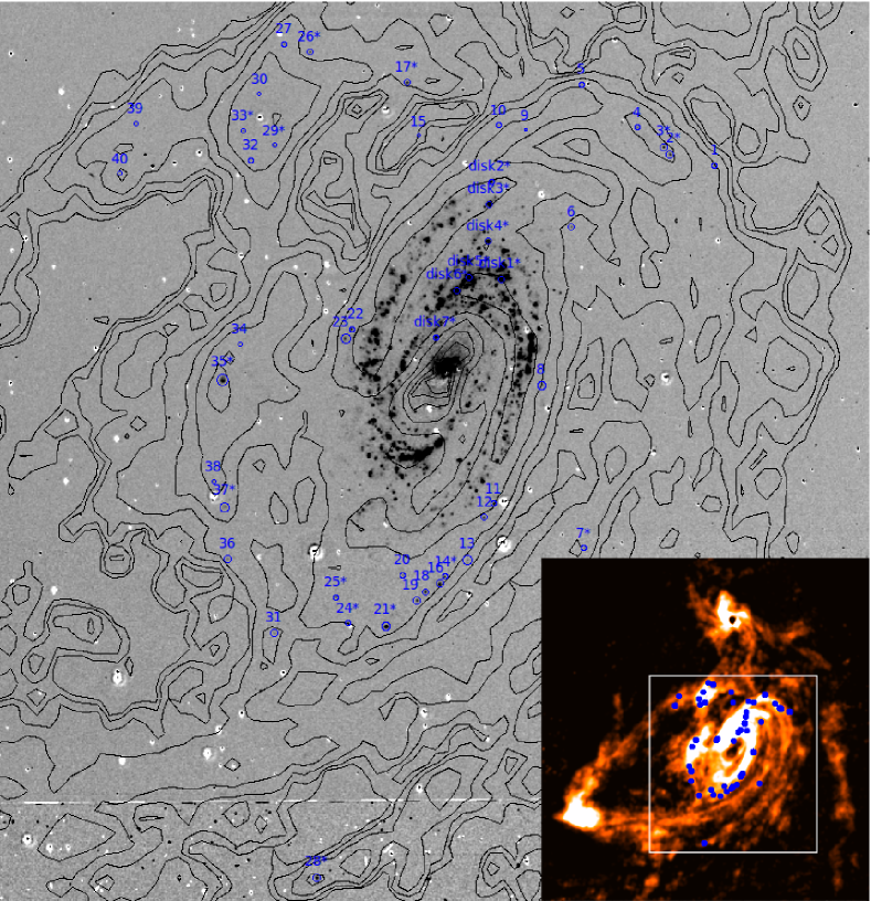
Figure 1: Burrell-Schmidt image of M81 in H$\alpha$ with the HII regions in our sample marked. The contours correspond to HI column densities of 1.8$\times$10²⁰ cm^-2 times 1, 2, 4, 8, 16, 32, and 64 from Yun, Ho & Lo (1994). HII regions with spectra are marked with asterisks. A list of all HII regions and their properties are provided in Table LABEL:tab:sample. In this paper, we discuss in particular region 21 (Münch 1), region 28 (the HII region near KDG 61), and region 35 (a bright ionized nebula near tidal dwarf candidate HoIX). In the bottom right corner, we show the HII regions marked on the full HI column density map of the M81-M82-NGC 3077 triplet, with the white box marking the size of the section of the Burrell-Schmidt H$\alpha$ image shown here.

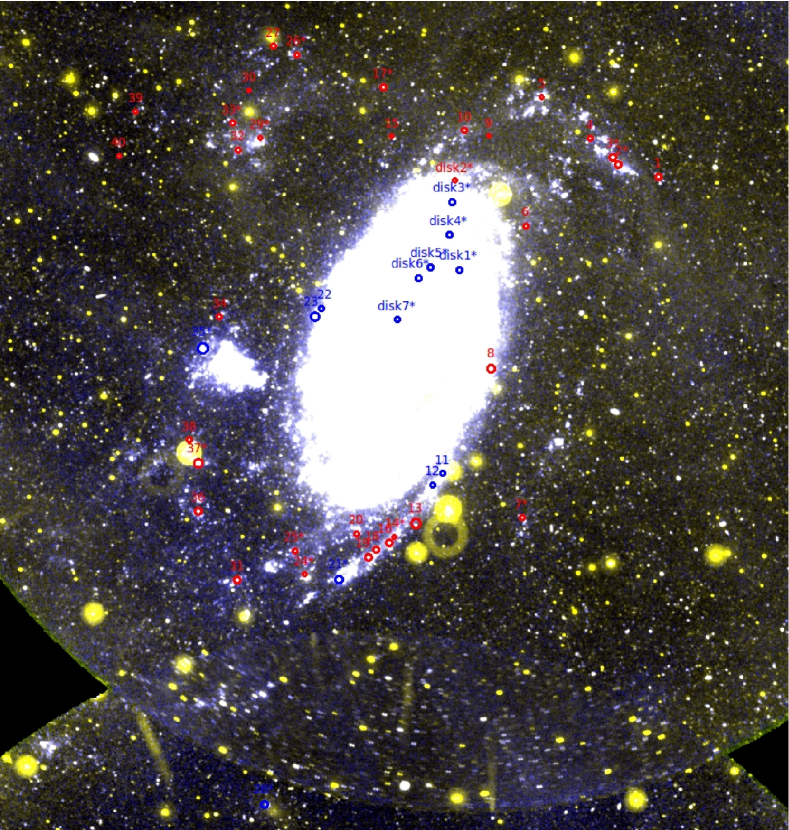
Figure 2: GALEX color-composite image shown on the same scale as the previous figure and with HII regions marked for comparison. We show GALEX FUV in blue, GALEX NUV in red, and an average of the two in green. The image is stretched to a square root scale in order to enhance the faint outer disk star forming features. The HII regions marked in blue signify previously catalogued objects, whereas the red regions denote newly found objects. Of particular interest is region 35, which is offset from the UV emission of the dwarf galaxy HoIX. We show a larger image of this object in Fig. 4.

Candidate HII regions were selected by visual comparison of the H$\alpha$ + [NII] image to the continuum image. We limited our search to a 42′$\times$63′ box centered on the galaxy center. We obtained fluxes for the HII regions within an appropriately sized circular aperture chosen individually for each region. The aperture size for each HII region was chosen to have a radius just large enough so that the enclosed flux profile flattened sufficiently, meaning that the level of the background had been reached. We subtracted the background level as determined from a small annulus around each aperture. The average aperture size of our HII regions is $\sim$9.5^′′, which corresponds to a physical size of 170 pc. This is approximately the same size as the faintest ($\log(L_{H\alpha})$$\sim$37.3) outer disk HII regions described by Ferguson, Gallagher & Wyse (1998). Only candidate regions with signal to noise greater than 4 were kept, setting our detection limit to $\log(L_{H\alpha})$$\sim$36.6. Note that this is brighter than the expected H$\alpha$ luminosity for the faintest single star HII regions ($\log(L_{H\alpha})$$\sim$36.15-36.30 for a B0.5 star (Vacca, Garmany & Shull, 1996; Sternberg, Hoffmann & Pauldrach, 2003)). The faintest HII regions detected here are the equivalent of what is predicted for a single ionizing O9 star (Sternberg, Hoffmann & Pauldrach, 2003). We found 40 HII regions outside of the main disk at a 4$\sigma$ confidence level within a distance of $\sim$3$\times$$R_{25}$. The locations of our HII regions are shown in Figs. 1 and 2, in which we show the H$\alpha$ image as compared to HI (Yun, Ho & Lo, 1994) and GALEX UV data (Thilker et al., 2007). We verified our flux calibration by comparison with the fluxes of several HII regions in the main disk given by Lin et al. (2003) and Pérez-González et al. (2006), using the aperture sizes quoted in each paper. We estimate our absolute fluxes to be accurate to $\sim$9%, based on the uncertainties of Lin et al. (2003) and Pérez-González et al. (2006) and the uncertainty in our calibration. To convert to H$\alpha$ luminosities, we assumed the [NII]/H$\alpha$ ratio to be 0.4 and a distance to M81 of 3.63 Mpc. In Table LABEL:tab:sample, we list the HII regions in our sample, noting their locations, galactocentric distances, sizes, and H$\alpha$ luminosities. For previously catalogued objects, we provide alternative names from Hodge & Kennicutt (1983), Miller & Hodge (1994), Petit, Sivan & Karachentsev (1988), Münch (1959), and C09.

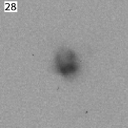
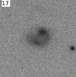
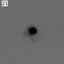
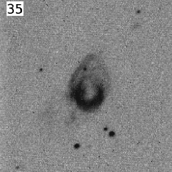
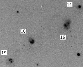
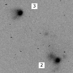
Figure 3: H$\alpha$ SPICAM images of several interesting HII regions. The red continuum light has not been removed in these images to show stars for reference. Top Left: HII region 28, associated with the dwarf spheroidal galaxy KDG 61 (not shown to the lower right.) It has a horseshoe shape morphology with a cavity-like feature to the north. Top Right: HII region 17, located to the north of M81 with a comma shape morphology. Middle Left: HII region 21 (Münch 1), a bright (1.5 $\times 10^{38}$ ergs s^-1) region in the Southern tidal arm of M81. It has two prominent loops of gas protruding from a bright central region. Middle Right: HII region 35, associated with the tidal dwarf HoIX, whose main body is outside this image to the lower right shown in full in Fig 4). It has a similar horseshoe morphology to KDG 61. The source within the shell just to the lower left of center is a star. Bottom Left: String of HII regions in the Southern tidal arm of M81. From left to right, region 19 has four visible knots of gas. Region 18 has a horseshoe shape similar to KDG 61 and HoIX. Region 16 has a very flocculent morphology. Region 14 appears smooth and round. Bottom Right: Two HII regions in the Northern tidal arm of M81. On the left, region 3 has a bright concentration with extended features. On the right, region 2 has a bright region with several flocculent tufts of gas.

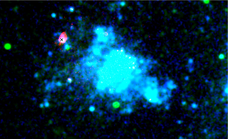
Figure 4: Three color image using the SPICAM continuum subtracted H$\alpha$ image (red) combined with GALEX FUV (blue) and NUV (green) of Holmberg IX and the HII region referred to here as region 35. Note that the bright HII region is offset from the main body of the dwarf galaxy, though there is a peak in the UV emission within the lower central part of the HII region. The HII region does, however, lie within a peak in the HI column density map, as can be seen in Fig. 1. The ’x’ marks the location of the x-ray source HoIX X-1 (or M81 X-9), which is contained within the extent of the H$\alpha$ emission (Immler & Wang, 2001; Wang, 2002).

Higher resolution H$\alpha$ plus continuum images of several HII regions are included in Fig. 3 to show the morphologies of several interesting regions. We chose to show a few of the brightest HII regions located in various areas of the outskirts. These images were obtained with the SPICAM instrument on the Apache Point Observatory ARC 3.5-meter telescope. The full images have a 4.8$\times$4.8 arcmin² field of view and were obtained in 2$\times$2 pixel binning mode, giving 0.28 arcsec pixel^-1. The coverage of the SPICAM images was such that they overlapped with 36 of the Schmidt HII region detections; all those were confirmed. For each field, two 420 second H$\alpha$ exposures were taken with a 25Å (FWHM) filter. Two 60-90 second exposures in R band were also obtained for continuum imaging. In Fig. 4, we show an RGB image of region 35 and the dwarf galaxy HoIX, using continuum subtracted H$\alpha$ (red), GALEX NUV (green), and GALEX FUV (blue). This HII region is noticeably offset from the main body of the dwarf galaxy, which shows little H$\alpha$ emission. However, there is UV emission within this region, and, as shown in Fig. 1, the region lies in a peak of the HI. We will discuss this region extensively in a later section of this paper.

We obtained 21 spectra for HII regions in the disk and outskirts of M81 identified in the Burrell-Schmidt image using the Blue Channel spectrograph on the 6.5-meter MMT telescope over four nights in January 2002. The selected regions lie at various galactocentric distances from $\sim$3 to 33 kpc and range in log($L_{H\alpha}$) luminosity from $\sim$36.9 to 38.9 ergs s^-1. HII regions for which we have spectra are marked in Fig. 1 with asterisks. We observed with a 500 mm^-1 grating, covering the wavelength range from 3650-7150 Å with a dispersion of 1.19 Å pixel^-1. We used a 2″$\times$180″ slit aligned along the average parallactic angle for each observation. The final spectral resolution is 7 Å FWHM. The CCD camera produced 3072 pixel (wavelength) $\times$ 220 pixel (spatial) images with 0.56″ per pixel spatial scale (after two pixel binning only in the spatial direction). Each night we observed a quartz lamp for flatfielding, twilight exposures for illumination correction, a Helium Neon Argon lamp for wavelength calibration, and 4-5 standard stars for flux calibration. For objects with spectra, the exposure times are noted in the last column.

2.2 Spectroscopic Data Reduction

We used the iraf task ccdproc to remove overscan, trim, and flatfield all the MMT spectra (Tody, 1993). We applied a slit illumination correction to the data derived from twilight exposures frames. A $\sim$4% gradient along the spatial axis was typically present before the twilight correction. To remove cosmic rays, we averaged frames for each object using imcombine with the cosmic ray reject option (crreject) enabled. All 2-D spectra were wavelength calibrated using a Helium Neon Argon image taken near the rotation angle of each science exposure. The spectrum of each object was extracted using an appropriate size aperture based on a visual inspection of the spatial extent of each target. A standard star spectrum was used as a reference for the trace along the dispersion axis if the HII region continuum was too weak to use as a trace. We flux calibrated all spectra using a separate sensitivity function for each of the four nights made from at least four standard star observations. The 1$\sigma$ uncertainty introduced in the absolute flux calibration for the first three nights is $\sim$3%, across the wavelength range. The uncertainty in our absolute flux calibration for the fourth night of observations is $\sim$6%, slightly higher due to varying weather conditions.

To correct for interstellar reddening, we used the iraf task deredden, assuming R=3.1 and using the reddening law from Cardelli, Clayton & Mathis (1989). We derived the logarithmic extinction at H$\beta$, $c(H\beta)$, for each spectrum using the observed H$\alpha$ to H$\beta$ ratio and taking an intrinsic value of H$\alpha$/H$\beta$= 2.86, which assumes photoionization and Case B recombination (Osterbrock & Ferland, 2006). Note, however, that this assumption may be not be valid for region 35, which harbors the ultraluminous x-ray source M81 X-9. We will address the effect of shock ionization on the abundance for this object specifically in §4. The uncertainty in our extinction correction was calculated by propagating the errors in the H$\alpha$ and H$\beta$ lines. Because the underlying continuum was very weak in most of our objects, the Balmer line fluxes were not corrected for stellar absorption. We measured the flux in each detectable line of our dereddened spectra with a Gaussian fit to the line profile using the task splot. The final errors in our dereddened line fluxes are due to a combination of uncertainties from our flux calibration, the line flux measurements with splot, and the extinction correction. Our dereddened line fluxes relative to H$\beta$ and extinction coefficients for a subset of emission lines are listed in Tables 2 and 3. In the last line of each table, we also mark the regions which have Wolf-Rayet features in their spectra, such as the 4660Å blue bump or emission at HeII $\lambda$4686.

3 Oxygen Abundances

We derive oxygen abundances for HII regions in our sample using two different methods. The first method is a “direct” method, using temperature sensitive emission lines to constrain the oxygen abundance. Because this method requires measuring very weak lines, we were able to calculate an oxygen abundance for only seven HII regions in our sample. We describe our determination of oxygen abundances from electron temperature lines in §3.1.

The second method, which we describe in §3.2, uses strong lines to constrain the oxygen abundance without directly measuring the electron temperature. Although this is an indirect method for abundance determination, the strong line calibrations allow us to derive an oxygen abundance for all HII regions in our data set. We use two $R_{23}$ based metallicity calibrations and two metallicity calibrations based on the [NII]/[OII] ratio. Because the $R_{23}$ parameter is a non-monotonic function of metallicity, we must first decide whether each region lies on the upper or lower branch of the $R_{23}$ vs. metallicity relation. We describe the upper vs. lower branch determination in §3.2.1. Having determined each region’s branch placement, we then use two separate strong line $R_{23}$ calibrations to derive oxygen abundances in §3.2.2. In §3.2.3, we derive strong line abundances using the [NII]$\lambda$6584/[OII]$\lambda$3727 ratio and compare these results to our $R_{23}$ based abundances. We mark abundances determined from electron temperatures distinctly from our strong line abundances throughout plots in the next sections for easy comparison. For a thorough discussion of a comparison of methods of abundances determination see Kennicutt, Bresolin & Garnett (2003).

3.1 Electron Temperature Abundances

For seven of our HII regions, we were able to derive electron temperatures using either the [NII] ($\lambda$6583 and $\lambda$5755) or [OIII] ($\lambda$5007 and $\lambda$4363) lines. Note that there may be some bias as to the metallicities of the regions with detectable electron temperature lines. HII regions with higher abundances will have lower electron temperatures and therefore more difficult to detect weak electron temperature lines. Yet, we are still able to derive electron temperature lines for regions between 5.7 to 32 kpc, which covers a larger radial range than any previous HII region metallicity study for M81.

We calculate the electron temperatures using the iraf task temden which calculates either temperature or density as part of the nebular package (Shaw & Dufour, 1995). The tasks in the nebular package are based on a 5-level atom program that approximates the physical conditions in a nebula, originally described by De Robertis, Dufour & Hunt (1987). Since the ratio of the [SII] lines $\lambda$6716/$\lambda$6731 $\sim$1.4 for all seven regions, we assume that $n_{e}$ is in the low density limit and is approximately 100 cm^-3. Table 4 gives the measured temperatures derived from [NII] and [OIII] lines in cases where these lines were detectable. Where these lines were not detected, we adopt temperatures derived using the following equations from Garnett (1992):

$$T(OII) =T(NII)$$ (1)

$$T(OII) =0.7T(OIII)+3000K$$ (2)

We then calculate oxygen ion abundances using the iraf task nebular.ionic. We used the flux from [OII]$\lambda$3727 for the O⁺/H⁺ calculation, and [OIII]$\lambda$5007 for the O⁺²/H⁺ calculation. Table 5 gives the derived oxygen ion and element abundances for the seven HII regions with detectable electron temperature lines. The errors in the abundances are dominated by uncertainty in the adopted temperatures.

3.2 Strong Line Abundances

Most of the HII region spectra do not have strong enough [OIII]$\lambda$4363 or [NII]$\lambda$5755 lines to derive reliable temperatures for abundance determinations. We use both $R_{23}$ based and [NII]/[OII] ratio based metallicity calibrations to derive oxygen abundances for all HII regions in our sample.

First, we discuss abundances based on the metallicity-sensitive parameter $R_{23}$ (Pagel et al., 1979), which is defined as the flux ratio of lines as follows:

$$R_{23}\equiv\frac{[OII]\lambda 3727+[OIII]\lambda\lambda 4959,5007}{H\beta\lambda 4861}$$ (3)

The main advantage of using the $R_{23}$ parameter as an indication of oxygen abundance is that it is a direct function of the strength of the lines for the first and second ionization states of oxygen, rather than depending on line ratios of other elements. To use the $R_{23}$ parameter, we must decide a priori whether the HII region is on the upper or lower branch of the $R_{23}$ to O/H relation.

3.2.1 Upper or lower $R_{23}$ branch?

We use both the [NII]$\lambda$6584/[OII]$\lambda$3727 and [NII]$\lambda$6584/H$\alpha$ ratios to break this upper vs. lower branch degeneracy, comparing the methods of Contini et al. (2002) and Kewley & Ellison (2008). From Contini et al. (2002), HII regions with

$$\log\left(\frac{\mbox{[NII]}}{\mbox{[OII]}}\right)>-1.05\mbox{~{}~{}~{}and~{}~{}~{}}\log\left(\frac{\mbox{[NII]}}{\mbox{H}\alpha}\right)>-1$$ (4)

lie on the upper branch, and HII regions with

$$\log\left(\frac{\mbox{[NII]}}{\mbox{[OII]}}\right)<-0.8\mbox{~{}~{}~{}and~{}~{}~{}}\log\left(\frac{\mbox{[NII]}}{\mbox{H}\alpha}\right)<-1$$ (5)

lie on the lower branch. Kewley & Ellison (2008), however, choose a division between the upper and lower branches at the following values:

$$\log\left(\frac{\mbox{[NII]}}{\mbox{[OII]}}\right)\sim-1.2\mbox{~{}~{}~{}and~{}~{}~{}}-1.3<\log\left(\frac{\mbox{[NII]}}{\mbox{H}\alpha}\right)\lesssim-1.1$$ (6)

We plot the values of these line ratios for all regions and overlay the branch divisions of Contini et al. (2002) as dashed lines and Kewley & Ellison (2008) as dotted lines in Fig. 5. Using these line ratio cuts, most of the HII regions in our sample lie unambiguously on the upper branch of the $R_{23}$ vs. O/H relation, according to both methods. None of the regions in our sample lie on the lower branch. Four of the regions, however, lie on the lower branch according to Contini et al. (2002) and on the upper branch according to Kewley & Ellison (2008). We mark these ambiguous regions as “turnaround” (T) regions and keep them separately visible in all figures. We note that two of these T regions do have an electron temperature derived abundance. We will address our treatment of these T regions in the next section.

3.2.2 $R_{23}$ Metallicity Calibrations

In order to derive oxygen abundances from the $R_{23}$ parameter, we calculated 12+log(O/H) using two methods, an “empirical” and a “theoretical” calibrations. Because theoretical calibrations generally overestimate oxygen abundances and empirical calibrations underestimate them (Kennicutt, Bresolin & Garnett, 2003), we derive abundances using two methods, one theoretical calibration and one empirical calibration, following the procedure described in Moustakas et al. (2010). The empirical calibration used is based on the oxygen abundances of observed HII regions directly determined from temperature sensitive lines from Pilyugin & Thuan (2005), hereafter PT05. The theoretical calibration used is based on the relationship between line strengths and metallicity from photoionization models of HII regions from Kobulnicky & Kewley (2004), hereafter KK04.

For the empirical abundance calibration, we have the following equations from PT05 for the upper and lower branches of the $R_{23}$ vs. O/H relation:

$$12+\log{\mbox{(O/H)}}_{\mbox{lower}}=\frac{R_{23}+106.4+106.8P-3.40P^{2}}{17.72+6.60P+6.95P^{2}-0.302R_{23}}$$ (7)

and

$$12+\log{\mbox{(O/H)}}_{\mbox{upper}}=\frac{R_{23}+726.1+842.2P+337.5P^{2}}{85.96+82.76P+43.98P^{2}+1.793R_{23}},$$ (8)

where

$$P\equiv\frac{\mbox{[OIII]}\lambda\lambda 4959,5007}{\mbox{[OII]}\lambda 3727+\mbox{[OIII]}\lambda\lambda 4959,5007}.$$ (9)

In Table 6, we list our calculated values of 12+log(O/H) via this method as well as the values of $P$ for each region.

For the theoretical abundance calibration, we have the following equations from KK04:

$$12+\log{\mbox{(O/H)}}_{\mbox{lower}}=9.40+4.65x-3.17x^{2}-\log(q)(0.272+0.547x-0.513x^{2})$$ (10)

and

$$12+\log{\mbox{(O/H)}}_{\mbox{upper}}=9.72-0.777x-0.951x^{2}-0.072x^{3}-0.811x^{4}\\ -\log(q)(0.0737-0.0713x-0.141x^{2}+0.0373x^{3}-0.058x^{4}),$$ (11)

where $x\equiv\log(R_{23})$ and $q$ is the ionization parameter given by

$$\log(q)=[32.81-1.153y^{2}+z(-3.396-0.025y+0.1444y^{2})]\\ \times[4.603-0.3119y-0.163y^{2}+z(-0.48+0.0271y+0.02037y^{2})]^{-1}$$ (12)

in units of cm s^-1. In these equations $z\equiv 12+\log$(O/H), $y\equiv\log$(O₃₂), and

$$\mbox{O}_{32}\equiv\frac{\mbox{[OIII]}\lambda\lambda 4959,5007}{\mbox{[OII]}\lambda 3727}.$$ (13)

The 12+log(O/H) formulas for both the upper and lower branches of this calibration are a function of $\log(q)$, which is dependent upon 12+log(O/H), requiring an iterative calculation to converge upon a solution. We were able to derive an $R_{23}$ oxygen abundance from this calibration for all HII regions in our sample. Our values of 12+log(O/H) and $O_{32}$ from this calibration are listed in Table 6.

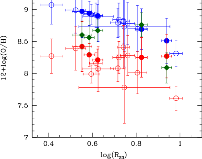
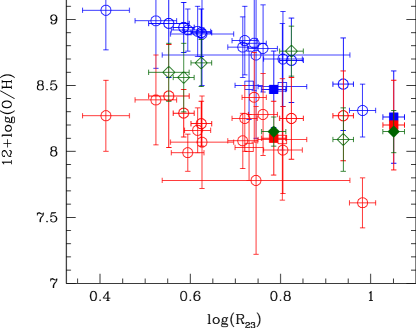
Figure 6: In the top graph, we show $R_{23}$ vs. 12+log(O/H) for the HII regions in our sample that lie on the upper branch. We show the values for 12+log(O/H) derived with the KK04 (Kobulnicky & Kewley, 2004) method (blue) vs. the PT05 (Pilyugin & Thuan, 2005) method (red). The filled green diamonds and the filled circles show the temperature derived abundances and the strong line abundances, respectively, for the same HII region. The KK04 calibration gives a higher upper branch than the PT05 calibration. In the bottom graph, we now include the turnaround regions here as squares. Two turnaround HII regions also have temperature derived abundances, and we mark all derived metallicities for these two objects with filled points.

In Fig. 6, we plot the $R_{23}$ vs. metallicity relation for our HII regions for both the theoretical KK04 and empirical PT05 metallicity calibrations. In the top graph, we are showing only the HII regions on the upper branch, to compare the two calibrations. The KK04 strong line metallicity calibration gives an upper branch on the $R_{23}$ vs. metallicity relation that lies higher than the PT05 strong line metallicity calibration. The solid points mark upper branch HII regions that have both a temperature derived metallicity (filled diamonds) and a strong line metallicity (filled circles). The temperature derived metallicities are in agreement with the KK04 and PT05 metallicities, within errors, though are, on average, between the two calibrations.

For each turnaround (T) region, we average the upper and lower branch solutions of the KK04 calibration and average the upper and lower solutions of the PT05 calibration to get a turnaround metallicity estimate from each calibration. In the bottom graph of Fig. 6, we plot the final abundances for all regions, with the T regions as squares on the $R_{23}$ vs. O/H relation. The filled points again mark two T HII regions with both a strong line metallicity and a temperature metallicity. Here, the temperature metallicities agree with both strong line abundances, within the errors, but may be in closer agreement with the PT05 derived abundances. In Table 6, we list the values of $R_{23}$ for each region and mark which branch we assume each region lies on.

3.2.3 [NII]/[OII] Metallicity Calibrations

In addition to the two $R_{23}$ based strong line metallicity calibrations, we also use two calibrations based on the [NII]$\lambda$6584/[OII]$\lambda$3727 lines flux ratio. While we used the [NII]/[OII] ratio to determine the upper and lower branches of the $R_{23}$ vs. metallicity relation, the [NII]/[OII] ratio is itself also a function of metallicity. Additionally, it does not suffer from the upper and lower branch ambiguity of the $R_{23}$ calibrations, since it is a monotonic function.

The first calibration we use is a theoretical calibration based on photoionization and stellar population synthesis models of Kewley & Dopita (2002), hereafter KD02, as follows:

$$\log{\mbox{([NII]/[OII])}}=1106.87-532.154Z+96.3733Z^{2}-7.81061Z^{3}+0.239282Z^{4},$$ (14)

where $Z=12+\log{\mbox{(O/H)}}$. This equation assumes ionization parameter $q$ = 2 $\times$ 10⁷ cm s^-1, which is appropriate given the range of ionization parameters for our sample ($\sim$ 1-7 $\times$ 10⁷ cm s^-1). To find values of $Z$, we use the IDL task fz_roots, based on the numerical recipe zroots (Press et al., 1992) which finds the roots of an $n$-order polynomial. We list the values of log([NII]/[OII]) and oxygen abundances derived using this calibration in Table 6. Since the two lines are strong, the errors are dominated by a systematic error of $\sim$0.1 dex given by the rms of the line fit defining the calibration. The abundances we derive from this calibration agree most closely with the KK04 $R_{23}$ abundances, which is not surprising since both calibrations are based on the same models. This calibration is simpler than that of KK04, however, since we do not explicitly calculate an ionization parameter for each HII region, but assume one appropriately chosen value for all.

We also use an empirical calibration from Bresolin (2007), hereafter B07, based on data from a number of HII regions with electron temperature abundances:

$$12+\log(\mbox{O/H})=8.66+0.36x-0.17x^{2},$$ (15)

where $x=\log(\mbox{[NII]/[OII]})$. Here the errors again are dominated by the systematic error of $\sim$0.2 dex from the rms of the fit to the log([NII]/[OII]) metallicity relation. We list the values of 12+log(O/H) from this calibration in Table 6.

The various calibrations all seem to have different metallicity scales (i.e. they are offset from each other). We will therefore focus in our discussion on the metallicity gradients implied by each of them in §5.

4 Holmberg IX and KDG 61

Several objects in our sample deserve special discussion. These include the brightest ionized nebula near the claimed tidal dwarf candidate Holmberg IX (region 35 in our labeling), a bright HII region near KDG 61 (region 28), and Münch 1 (region 21). We will discuss Münch 1 in the next section.

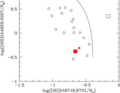
Figure 7: BPT diagram (Baldwin, Phillips & Terlevich, 1981) of our HII region data (open points) compared with three data points (filled) from C09 (Croxall et al., 2009). The curved line marks the empirical division between HII region-like objects (to the lower left) and AGN (upper right), taken from Osterbrock & Ferland (2006). The two triangles mark our region 28 (or KDG 61-9). Both our data and that of C09 show a highly excited HII region. The square points mark the bright ionized gas region associated with HoIX (MH9/MH10). Our data for this region shows evidence of shock ionization, whereas the data of C09 does not. We attribute this to the spatial offset of our long-slit spectrum as compared to the GMOS spectrum of C09, and the complex ionization conditions in this large object.

The large object near the dwarf galaxy Holmberg IX was first identified in H$\alpha$ imaging by Miller & Hodge (1994) as three HII regions- MH9, MH10, and MH11. We show an H$\alpha$ plus continuum image of the entire object (our region 35) in Fig. 3 and an RGB image combining H$\alpha$ (red), GALEX NUV (green), and GALEX FUV (blue) of the HII region and the dwarf galaxy HoIX in Fig. 4. From the image in Fig. 4, it is obvious that the bright H$\alpha$ emission is offset from the main body of the dwarf galaxy, but coincides with a peak in the HI distribution (see Fig. 1). Studies of Holmberg IX suggest that the dwarf galaxy itself has a tidal origin, given its location in the tidal HI streams and young stellar population dominated by stars less than $\sim$200 Myr old, which is consistent with star formation triggered by the past interaction of M81 and M82 (Sabbi et al., 2008; Weisz et al., 2008; Hoversten et al., 2011). The nature of the large ionized object is discussed in Miller (1995) as a U-shaped “supershell” approximately 250 pc wide and 475 pc in the north-south dimension, with strong [SII], [NII], [OI], and [OII] emission indicative of shock heating. The supershell is the optical counterpart of the x-ray source ULX HoIX X-1 (M81 X-9) (Fabbiano, 1988). In Fig. 4, we mark the location of the x-ray source, which is nested in the lower eastern portion of the “U” shape and appears to be confined within the spatial extent of the H$\alpha$ emission (Immler & Wang, 2001; Wang, 2002). A recent HST/ACS study by Grisé et al. (2011) finds an OB association of young stars ($\lesssim$20 Myrs) in MH10. C09 find an oxygen abundance of 12+log(O/H)=8.91$\pm$0.20 for this HII region (called UGC 5336-3 in that paper), using a strong line calibration from McGaugh (1991). The data comes from the Gemini Multiple Object Spectrograph (GMOS) and is focused on the lower eastern section of the “U”. The slit of our spectrum for this object was aligned so as to include both MH9 and MH10, both halves of the “U”. We find lower abundances of 12+log(O/H) = 7.61$\pm$0.19 (PT05), 8.31$\pm$0.20 (KK04), 8.68$\pm$0.10 (KD02), and 8.21$\pm$0.20 (B07). These theoretical model based calibrations assume that the emission is solely due to photoionization, but the strong [SII] emission in our data suggests the presence of some shock ionization. In Fig. 7, we plot a BPT emission line diagnostic diagram (Baldwin, Phillips & Terlevich, 1981) showing the [OIII] and [SII] emission lines normalized to Balmer lines for our HII regions, as well as the data of C09. Our line ratios indeed place the section of the object we observed in the shock excited range, but note that the C09 data are not in that same section. Clearly, this object appears to be a complex mixture of H$\alpha$ emission from both photoionization and shock ionization. We compare our line ratios to the shock models of Allen et al. (2008) and find that our data is consistent with a low velocity shock ionized region with a 12+log(O/H) metallicity between that of the LMC (8.35) and solar (8.93), which is in agreement with the abundances we derive using the KK04 and KD02 methods. The data of C09 for this region does not show evidence of shock ionization. We take the emission line fluxes from the C09 data and re-calculate strong line abundances of 8.21$\pm$0.16 (PT05), 9.02$\pm$0.18 (KK04), 8.76$\pm$0.10 (KD02), and 8.30$\pm$0.20 (B07). The (KD02) calibration of the C09 data for this object is most consistent with the metallicity of our data assuming some shock ionization for this region.

We also observe an HII region near the dwarf galaxy KDG 61, region 28 in our data (see Fig. 3) and KDG 61-9 in C09. This object is a highly ionized object with strong [OIII] emission as shown in Fig. 7. Like C09, we also detect the emission line HeII $\lambda$4686 which indicates that this object may have a central Wolf-Rayet star. We derive an electron temperature oxygen abundance of 8.15$\pm$0.11 and strong line abundances of 8.20$\pm$0.34 (PT05), 8.26$\pm$0.35 (KK04), 8.71$\pm$0.10 (KD02), and 8.24$\pm$0.20 (B07) for this object. C09 report an electron temperature abundance of 8.35$\pm$0.05, which is slightly higher than our value, since we measure T[OIII] to be $\sim$1800 K higher. Makarova et al. (2010) find a radial velocity for the stellar light of KDG 61 of +221$\pm$3 km s^-1, whereas for this HII region they find a velocity of $-$123$\pm$6 km s^-1. From the velocities, the authors conclude that this HII region is not bound to the dwarf spheroidal galaxy and is likely a chance projection. This region marks one of the most distant points in our abundance gradient, and its oxygen abundance is comparable to that of other regions at its radial distance. If we compare our abundance results for this region to the expected abundance for the dwarf galaxy KDG 61, we find higher abundances than what would be estimated from the metallicity-luminosity relation for dwarf galaxies (see e.g., Skillman, Kennicutt & Hodge, 1989). For a low luminosity dwarf like KDG 61, with $M_{B}$=-12.83$\pm$0.30 (Karachentsev et al., 2004), C09 shows that the metallicity-luminosity relation for dwarf galaxies in the M81 group predicts an oxygen abundance of $\sim$7.6. We agree with C09 that the abundance of this region is more consistent with an origin in enriched gas from the tidal interactions of M81 rather than from the dwarf galaxy KDG 61. We will discuss in detail the possible effects of M81’s interaction history on the abundances of the outer disk and the abundance gradient in §6.

5 Abundance Gradient

To obtain deprojected distances for all HII regions in our sample, we assume a flat planar geometry, with a rotation angle of 157^∘ and an inclination angle of 59^∘ for M81 (Kong et al., 2000). Clearly, the assumption of a planar geometry with the same orientations as the M81 disk may be incorrect for the outermost HII regions, given the role of tidal interaction in creating the HI tails. However, our regions do not probe all of the tidal tails and do not stray very far from M81 proper. For regions along the southern- and northern- most spiral arms, the deviation from the M81 disk is probably minor. The southern arm extends into the HoIX region (see Fig. 1, our region 35.) The regions where the radial distance to M81 is most uncertain then likely include 26, 29, and 33 (all in Arp’s loop), and region 28 (near KDG 61). The latter is near the projected major axis of M81, so its actual radial distance from M81 cannot be less than the one we use. In the subsequent presentation of the radial abundance gradient, it is good to keep in mind that these regions are the four outermost points in radial distance. We will use our electron temperature and $R_{23}$ abundance determinations to discuss the metallicity gradient out to $\sim$2.25$\times$$R_{25}$, or $\sim$33 kpc from the center.

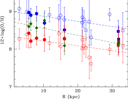
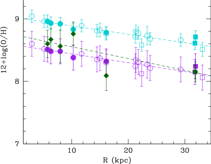
Figure 8: 12+log(O/H) vs. galactocentric distance for the HII regions in our data set. In the top graph, we show the metallicities from both $R_{23}$ calibrations as compared to the electron temperature metallicities. Blue points mark the abundances from the KK04 calibration, and red points mark the abundances from the PT05 calibration. Turnaround regions are marked by squares. Green diamonds show the temperature derived abundances. The strong line abundances that also have a temperature derived abundance are marked with filled circles. Münch 1 is marked by the green diamond at $\sim$16 kpc and the corresponding filled circles of the strong line abundances. The dashed lines show our weighted least-squares fit to the $R_{23}$ abundances and temperature abundances. In the bottom graph, we compare the abundances from the KD02 (Kewley & Dopita, 2002) and B07 (Bresolin, 2007) [NII]/[OII] metallicity calibrations to the temperature derived abundances. The slopes of the abundance gradients derived from all four strong line methods are roughly the same. The temperature derived abundance gradient is slightly steeper.

In the top graph of Fig. 8, we show abundance gradients from both the KK04 and PT05 strong line $R_{23}$ metallicity calibrations as well as the electron temperature abundances for the HII regions in our sample. The strong line abundances derived from the KK04 calibration are higher but show a gradient with a slope similar to the abundance gradient derived using the PT05 calibration. We use a weighted least-squares fitting routine with uncertainties in both error and distance and derive a gradient of $\Delta(\log$(O/H))$/\Delta$R${}_{G}=-$0.014$\pm$0.006 dex kpc^-1 from the KK04 abundances and $\Delta(\log$(O/H))$/\Delta$R${}_{G}=-$0.013$\pm$0.006 dex kpc^-1 from the PT05 abundances. The abundance gradient from electron temperature derived abundances is slightly steeper than those of the $R_{23}$ based calibrations, with a gradient of $\Delta(\log$(O/H))$/\Delta$R${}_{G}=-$0.020$\pm$0.006 dex kpc^-1. In the bottom graph of Fig. 8, we plot our abundance gradient derived from the [NII]/[OII] based calibrations of KD02 and B07 compared again to our electron temperature abundance gradient. We find a metallicity gradient of $\Delta(\log$(O/H))$/\Delta$R${}_{G}=-$0.013$\pm$0.002 dex kpc^-1 from the KD02 abundances and $\Delta(\log$(O/H))$/\Delta$R${}_{G}=-$0.014$\pm$0.005 dex kpc^-1 from the B07 abundances, similar to the gradients given by both $R_{23}$ metallicity calibrations. The four strong line abundance calibrations all give a consistently shallow negative metallicity gradient. Of the two $R_{23}$ metallicity calibrations we use, the PT05 abundances appear to be in closer agreement to our electron temperature abundances. The B07 [NII]/[OII] calibration gives the strong line abundances closest to the electron temperature abundances of our data set.

We compare our results with previously published HII region abundance results from GS87, S10, and three regions from C09, which studied the abundances of HII regions in M81 dwarfs. Two of these HII regions are located near Holmberg IX (UGC5336-3 and UGC5336-12), and the third is located near KDG 61 (KDG 61-9, also our region 28). The abundances quoted in S10 are derived from the electron temperatures from one or both of the [NII] and [OIII] lines. Where only one of the lines is detected, the authors assume the same temperature for all ions. In GS87, the authors use a theoretical calibration of the $R_{23}$ parameter from photoionization models. For the HII regions we include here from the data set of C09, the authors derive an electron temperature abundance for KDG 61-9 and use an $R_{23}$ calibration from McGaugh (1991) for the two regions near HoIX.

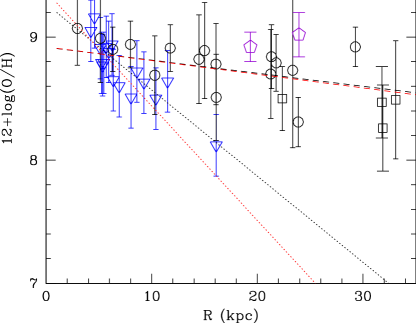
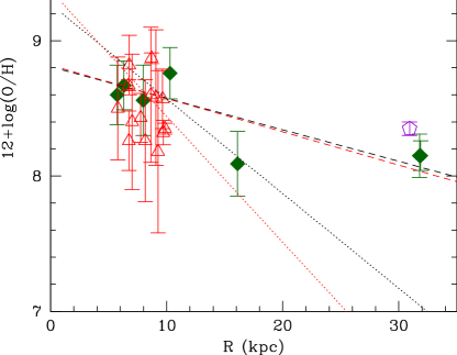
Figure 9: 12+log(O/H) vs. galactocentric distance for all HII regions including previous abundance work using the published values in those papers. We plot the abundances for our HII regions derived from the method most similar to the methods used in previous studies. In the top graph, we compare abundances published by C09 and GS87 (Garnett & Shields, 1987), which both use $R_{23}$ based photoionization models, with the abundances for our HII regions derived using the KK04 calibration. Münch 1 is marked by the blue triangle at $\sim$16 kpc, and the lower abundance black circle at the same radius. In the bottom graph, we compare electron temperature based abundances from S10 (Stanghellini et al., 2010) and C09, with the electron temperature based abundances from our HII regions. The dashed lines are our fits to all points shown, taking only our data if the HII region overlaps with another data set. The dotted lines shows the gradient derived by S10, which fit HII regions from both S10 and GS87 in the inner 17 kpc. (Red represents the fit from the routine fitexy (Press et al., 1992), and black represents a weighted least-squares fit.)

Because different methods of abundance calculations may yield different absolute abundances, in order to compare our abundances with previously published abundances, we separate the results into groups derived by similar methods. In the top graph of Fig. 9, we compare the published abundances from GS87 and C09 with the KK04 strong line abundances from our data set, since these abundances were all derived using the $R_{23}$ parameter and a theoretical calibration based on photoionization models. If we perform a weighted least-squares fit to this group of data, using only our abundance result if a region is in multiple data sets, we find a gradient of $\Delta(\log$(O/H))$/\Delta$R${}_{G}=-$0.011$\pm$0.005 dex kpc^-1. In the bottom graph of Fig. 9, we plot only HII regions with electron temperature derived abundances, using our data and the abundances published in S10 and C09. A weighted least-squares fit to these points gives a gradient of $\Delta(\log$(O/H))$/\Delta$R${}_{G}=-$0.023$\pm$0.004 dex kpc^-1, but there is an obvious lack of radial coverage for these results, with only one object between 12 and 30 kpc. If these electron temperature based abundances are closer to true abundances than the $R_{23}$ derived ones, it may be the case that the abundances can be described by a broken gradient, with a drop in metallicity from 10 to 15 kpc and a flatter outer gradient. However, we have no temperature derived abundances in the 10 to 15 kpc range, and the HII region at 16 kpc, Münch 1, may be an anomalous point, which we will discuss later in this paper. S10 derive an abundance gradient using a composite data set of HII regions from their paper and HII regions published by GS87, over a radial range from 3 to 17 kpc. They find a noticeably steeper gradient of $\Delta(\log$(O/H))$/\Delta$R${}_{G}=-$0.093$\pm$0.02 dex kpc^-1 using the fitexy routine and a slightly less steep gradient of $\Delta(\log$(O/H))$/\Delta$R${}_{G}=-$0.07 dex kpc^-1 using a least-squares fit. We plot these lines for comparison in this figure. The steep gradient that S10 derive is based on the steeper inner gradient found by GS87 from $\sim$3 to 10 kpc and the low abundance of Münch 1 at 16 kpc. Note that the S10 regions are too limited in radial range to derive an inner gradient.

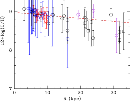
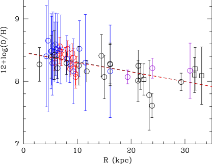
Figure 10: 12+log(O/H) from each strong line calibration vs. galactocentric distance for all HII regions including the reanalysis of previous data sets. Here, we rederive abundances for the HII regions in previous data sets using the same strong line $R_{23}$ based calibration for all regions. In the top graph, we calculate abundances for each HII region using the KK04 calibration. In the bottom graph, we derive abundances using the PT05 calibration. The dashed lines represent our weighted least-squares fits to all HII regions, taking only our data if the HII region overlaps with another data set.

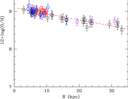
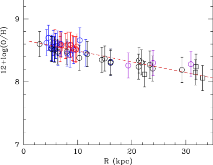
Figure 11: 12+log(O/H) vs. galactocentric distance derived from the [NII]/[OII] based calibrations of KD02 (top) and B07 (bottom) using the data in this paper and data from C09, S10, and GS87 reanalysed in the same method. The dashed lines are our fits to all points regions shown, taking only our data if the region falls in multiple data sets.

One important point to emphasize is that not all strong line calibration methods are alike. In the past decade, various refinements have been introduced. We therefore considered it useful to recalculate strong line abundances from previous data using the methods adopted in this paper. In Fig. 10, we have taken the emission line fluxes for the HII regions published by S10, GS87, and C09 and recalculated new strong line $R_{23}$ based abundances in the same way as for our data set, using again the two calibrations of KK04 and PT05. For the combined four data sets, using only our data if an HII region is also included in another data set, we find abundance gradients of $\Delta(\log$(O/H))$/\Delta$R${}_{G}=-$0.008$\pm$0.005 dex kpc^-1 from the KK04 calibration and $\Delta(\log$(O/H))$/\Delta$R${}_{G}=-$0.016$\pm$0.004 dex kpc^-1 from the PT05 calibration. The abundances given by the KK04 calibration for the HII regions in the data set from GS87 are closest to the published values in that paper. The GS87 data for Münch 1 also give a relatively low abundance for this calibration, as shown by the open blue circle near 16 kpc in Fig. 10. Our data for this object, marked by a black open circle at the same radius, shows a relatively low abundance derived from the KK04 calibration as compared to other objects near this distance. In Fig. 11, we have recalculated strong line abundances for all previous data using the [NII]/[OII] ratio based calibrations used for our data set. We find an abundance gradient of $\Delta(\log$(O/H))$/\Delta$R${}_{G}=-$0.016$\pm$0.002 dex kpc^-1 from the KD02 calibration and $\Delta(\log$(O/H))$/\Delta$R${}_{G}=-$0.017$\pm$0.004 dex kpc^-1 from the B07 calibration. The location of the points for the KD02 and B07 calibrations suggest that the two calibrations are essentially the same with only a zero point offset.

The new strong line abundances that we calculate for these data sets are consistent with the gradients derived for only our data. The reanalysis of these previous data with the four strong line abundance calibrations that we use yields oxygen abundances with relatively shallow gradients for M81. The flatter gradient that we derive is not a consequence of disagreements between our data and previous data, but a result of our reanalysis of previous data sets using recent strong line calibration methods. It is worth noting that in a recent abundance study of blue supergiants, which, like HII regions, trace the current metallicity of the interstellar medium, Kudritzki et al. (2011) also find a relatively shallow gradient of $-$0.034 dex kpc^-1 across the main disk of M81. This is only slightly steeper than the gradients we find here. The coefficients to our least-squares fits to the metallicity gradient for different methods and sets of data are listed in Table 7.

Our oxygen abundance gradient is noticeably less steep than the previously published gradient of M81 derived from HII regions. We attribute this partially to the limited radial range of HII regions of previous studies and the high electron temperature and low abundance derived for Münch 1, which has the largest galactocentric radius for previous M81 metallicity gradient studies. Further inspection of this HII region’s spectrum shows the presence of HeII $\lambda$4686, meaning that the region is being heated by a very hot central star. The spatial extent of the HeII $\lambda$4686 is centrally confined to not much further beyond the continuum of the central star. We had hypothesized that the temperature lines may also be restricted in spatial extent to the very core of the HII region, thus giving a very high temperature in the core of the region which would not reflect the temperature across the region in its entirety. However, we find that the temperature lines have the same spatial extent as H$\beta$, and therefore the high electron temperature we derive for this region is representative of the whole region. It is worth noting that the [OIII] line at $\lambda$4363 lies under a mercury sky line, but we believe our background subtraction to be reliable. This HII region compared to the more distant regions in our data set has an anomalously low oxygen abundance as derived from the electron temperature, as well as from the KK04 calibration on this object.

It is worth noting that the low abundance derived from electron temperature for Münch 1 may not be anomalous to this HII region, since we do not currently have spectra deep enough to derive oxygen abundances based on temperature sensitive lines for other HII regions at this radius ($\sim$10-20 kpc). More data are needed, particularly for the nearby string of HII regions in the outer southern tidal arm, to conclude whether this HII region is atypical in its low temperature derived oxygen abundance and to explore the possibility of a broken gradient. Though a continuously sloped gradient is a good fit to our strong line abundance gradients, they may be equally well-described by a slight brokent gradient, with a flattening past $\sim$16 kpc, such as the broken gradients seen in M83 (Gil de Paz et al., 2007; Bresolin et al., 2009) and NGC 4625 (Goddard et al., 2011).

The slope of the oxygen abundance gradient may also be affected by our averaging of the upper and lower branch metallicities for the HII regions which do not clearly lie on the upper or lower branch of the $R_{23}$ vs. metallicity calibration. These regions all lie at distances greater than $\sim$22 kpc from the galactic center. If we assume that these ambiguous regions lie on either the upper or lower branch, the values of 12+log(O/H) that we calculate are $\sim$0.25 higher or lower than our average metallicity, which would slightly change the slope of the abundance gradient. In particular, if we assume that these regions lie on the lower branch, the gradient could be steeper, or could be represented by a broken gradient, shallow in the main disk and dropping off to a flatter low abundance past $\sim$22 kpc. However, our favored interpretation is that the metallicities of these ambiguous regions are best represented by the average of the upper and lower branch values. These values appear to agree nicely with our final $R_{23}$ vs. (O/H) relation of both strong line abundances for the upper branch regions and our temperature derived abundances. Additionally, the gradient we derive from the [NII]/[OII] calibrations, which does not suffer from this metallicity degeneracy, are similar in slope to both $R_{23}$ based abundance gradients with these four turnaround regions.

6 Discussion

We have used four strong line calibrations in addition to electron temperatures to derive abundances for our HII regions, and while we find similar slopes to the abundance gradients from these different methods, the absolute abundance for a region may vary significantly depending on the method used. This study demonstrates the need for adopting robust and consistent abundance diagnostics to reliably determine abundance distributions in galaxies. Using the abundance gradients presented in the previous section, here we discuss the possibilities of a broken gradient, a single gradient as a result of chemical evolution, and a gradient as a result of M81’s interaction history.

On one hand, our data show good agreement between the slopes of abundance gradients derived from both strong line abundances and temperature derived abundances, with the exception of Münch 1. On the other hand, the reanalysis of data from S10, GS87, and C09 to derive new strong line abundances leads to a significantly flatter abundance gradient in the inner part, consistent with the gradient we find for the outer part. It is important to confirm this through more electron temperature based abundances. Because low metallicity regions have the strongest and most easily detectable electron temperature lines, our temperature based abundances may reflect a bias towards these low abundances. In the inner regions, this could amount to underestimating the slope of the abundance gradient. Additionally, if our temperature based abundance of Münch 1 is an accurate representation of the true abundance at its radius, it is possible that M81 may have a broken metallicity gradient, with the break just outside of the optical radius $R_{25}$, similar to the profile seen in M83. M83 shows a negative oxygen abundance gradient in the inner disk and a flattening just outside of the optical radius out to 2.6 times $R_{25}$ (Gil de Paz et al., 2007; Bresolin et al., 2009). It also has an extended UV (XUV) disk with recent star formation far into the outer disk (Thilker et al., 2005, 2007). Bresolin et al. (2009) attribute the abundance profile flattening in the XUV disk to its relatively unevolved state. The authors draw the analogy of the low gas surface density and low star formation environment in the galaxy outskirts to low surface brightness galaxies, which have a nearly constant oxygen abundance as a function of radius (de Blok & van der Hulst, 1998). M81 also has an XUV disk so it would not be unlikely for this galaxy to show a broken abundance profile that flattens outside of the optical radius.

While M81 may have a broken gradient, as discussed above, the present data are more consistent with a single shallow gradient. The shallow negative metallicity gradient derived from the oxygen abundances of M81 imply only a slightly higher metallicity at small galactocentric radii than into the outskirts of the galaxy far beyond the optical radius of the disk. The flatter gradient reported here for M81 is now consistent previous observational findings showing that flatter gradients are observed in early-type spirals (Zaritsky, Kennicutt & Huchra, 1994) and that this trend disappears when gradients are normalized to disk size. If we compare the metallicity gradient of M81, $\Delta(\log$(O/H))$/\Delta$R${}_{G}\sim-$0.013 to $-$0.020 dex kpc^-1 (or $\sim-$0.19 to $-$0.29 dex/$R_{25}$), to the gradient of the Milky Way as similarly derived from HII regions, $\Delta(\log$(O/H))$/\Delta$R${}_{G}\sim-$0.04 to $-$0.06 dex kpc^-1 (or $\sim-$0.45 to $-$0.68 dex/$R_{25}$) (Deharveng et al., 2000; Esteban et al., 2005; Rudolph et al., 2006; Rood et al., 2007), both galaxies show a similarly shallow negative sloping trend, with a slightly steeper gradient for the Milky Way.

Chemical evolution models of galaxy disks usually rely on four basic constraints: the exponential stellar profile, the gaseous profile, the star formation rate profile, and the abundance profiles of different elements (in external galaxies, most of the time, oxygen). From these observational constraints, chemical evolution models can infer the star formation histories of disk galaxies. In the 90’s, it was shown both for the Milky Way (e.g., Matteucci & Francois, 1989; Chiappini, Matteucci & Gratton, 1997; Boissier & Prantzos, 1999), and for other spiral galaxies (Molla, Ferrini & Diaz, 1997), that one way to reproduce these constraints is to assume a star formation history that is a function of galactic radius (i.e., more peaked in the inner parts and less efficient in the outer parts). Furthermore, these models explain the observed shallower abundance gradient in more luminous galaxies due to a faster formation of large spiral galaxies (see Molla, Ferrini & Diaz 1997 for a comparative study of seven nearby spirals; Chiappini, Romano & Matteucci 2003 for M101; Renda et al. 2005 and Yin et al. 2009 for M31, Marcon-Uchida, Matteucci & Costa 2010 for M33). A common interpretation is that the variation of the accretion timescale of gas onto the disk should also be a function of the galaxy mass in the sense that the most massive galaxies formed in the shortest timescale (Prantzos & Boissier, 2000; Mollá & Díaz, 2005). The flatter oxygen gradient reported in this work for M81 is more consistent with this scenario than was reported in previous works. For M81, an Sa galaxy with rotation velocity $V_{max}$ = 260 km s^-1 (Rohlfs & Kreitschmann, 1980), we would expect an oxygen abundance gradient of $\Delta(\log$(O/H))$/\Delta$R${}_{G}\sim-$0.04 (Mollá & Díaz, 2005) to $-$0.05 dex kpc^-1 (Prantzos & Boissier, 2000). In comparison, the gradient presented in S10 of $-$0.093 dex kpc^-1 is significantly steeper than these predictions, as the authors note. The gradient that we find in this paper, in the range of about $-$0.01 to $-$0.02 dex kpc^-1 depending on method, is shallower than that of the Milky Way, as expected, but even flatter than the chemical evolution models of Prantzos & Boissier and Mollá & Díaz predict. Note, however, that these models do not consider a gas threshold for star formation, and models computed including this would predict shallower gradients in the outer parts of galaxies (see e.g., Chiappini, Matteucci & Romano, 2001).

It is likely that the shallow gradient is partially a result of the interaction history of M81 with its companions. Yun (1999) describes a simulation of the tidal interaction between M81, M82, and NGC 3077, in which much of the gas presently in the near outskirts of M81 originated in its disk and was pulled out by the interactions with these two galaxies. In this scenario, the interactions between these galaxies may have served to flatten the metallicity gradient of M81. Recent numerical simulations of chemical evolution in galaxy interactions predict the flattening of radial metallicity gradients soon after the first passage of interacting galaxies, due to the radial redistribution of gas over the disk (Kewley, Geller & Barton, 2006; Rupke, Kewley & Barnes, 2010). Moreover, the slope of the metallicity gradient of an interacting galaxy does not seem to be a strong function of the initial gradient (Rupke, Kewley & Barnes, 2010). Though these authors did not include star formation in their interaction simulations, the models of Perez, Michel-Dansac & Tissera (2011), which include star formation and subsequent supernova feedback, confirm the result of a flattened metallicity gradient for interacting galaxies. In the central regions, they find interaction-induced dilution, lowering the metallicity. In the outer regions, both in situ star formation activity and metal-rich gas transported from the inner disk to the outer disk increase the metallicity. These processes would produce a flattened gradient in an interacting galaxy.

Recent observational studies have also explored the connection between interacting galaxies and abundance gradients. The possibility of a past interaction is invoked as a feasible explanation for the flat metallicity gradient observed in the blue compact dwarf galaxy NGC 2915 (Werk et al., 2010). A survey of galaxies in an early stage of strong interaction by Rupke, Kewley & Chien (2010) provide observational confirmation of the flattening of radial metallicity gradients in interacting galaxies. The authors find that interacting galaxies, on average, have metallicity gradients that are less than half as steep as non-interacting galaxies. Specifically, they find a median oxygen abundance slope of $-$0.041$\pm$0.009 dex kpc^-1, or $-$0.57$\pm$0.05 dex/$R_{25}$, for the 11 isolated galaxies in the control sample (including NGC 300 and M101) and a shallower median slope of $-$0.017$\pm$0.002 dex kpc^-1, or $-$0.23$\pm$0.03 dex/$R_{25}$, for the 16 interacting galaxies studied. If we compare our results for M81, we find that our derived oxygen gradient has the shallow characteristic of a typical interacting galaxy. Though these studies find flat gradients for interacting galaxies, it is important to note that isolated galaxies also display flat gradients. For example, in a study of a sample of 13 galaxies in the HI Rogues catalog, Werk et al. (2011) find flat oxygen abundance gradients out to large radii, and most, though notably not all, of the galaxies are interacting. Additionally, deep CMD studies of the isolated galaxies NGC 300 (Vlajić, Bland-Hawthorn & Freeman, 2009; Gogarten et al., 2010) and NGC 7793 (Vlajić, Bland-Hawthorn & Freeman, 2011) find flattened metallicity gradients into the outer disks of these galaxies. Inefficient star formation in the galaxy outskirts could also produce a flattened abundance profile. It may be the case that the gas in the outskirts of M81 was pre-enriched by inefficient outer disk star formation and would have also displayed a shallow abundance gradient prior to its interaction with M82 and NGC 3077. However, given the interaction history of M81 as traced by the HI gas and the recent observational studies and simulations of flattened gradients in interacting galaxies, it is probable that the shallow abundance gradient into the outskirts of M81 is at least partially a result of interaction with the companion galaxies.

7 Summary

We have presented H$\alpha$ luminosities for 40 HII regions outside the main disk of M81. We have also presented emission line fluxes for 21 HII regions ranging from $\sim$3-33 kpc from the galaxy center, corresponding to $\sim$2.3$\times$R₂₅. We calculated strong line oxygen abundances from two $R_{23}$ based metallicity calibrations and two [NII]/[OII] based calibration. We find that M81 has a shallow negative gradient of $\Delta(\log$(O/H))$/\Delta$R${}_{G}\sim$$-$0.013 to $-$0.016 dex kpc^-1. For seven HII regions, we were able to derive oxygen abundances using electron temperature sensitive [NII] or [OIII] emission lines. We find the temperature derived abundances gradient to be slightly steeper than our strong line abundance gradients with $\Delta(\log$(O/H))$/\Delta$R${}_{G}\sim$$-$0.020 dex kpc^-1. Our oxygen abundance gradients are noticeably less steep than previous results. We attribute this partially to the possible atypically low abundance of the most distant HII region in previous data sets, Münch 1. We calculate a lower oxygen abundance for this region than for any other region in our sample, and it is not clear if this is a true reflection of the average metallicity at its radial distance. More deep spectroscopic data is needed for HII regions near Münch 1 to determine whether or not this region has an anomalously low metallicity and whether M81 shows a broken abundance profile with a flat outer disk gradient. Our shallow gradient is corroborated by our reanalysis of previous data. We combine our data with three published HII region data sets and recalculate oxygen abundances using a consistent strong line method for all data. The reanalysis of these data show a flatter gradient for M81. The shallow gradient may be flatter than some chemical evolution models predict for a galaxy of M81’s Hubble type and mass. This may be explained by radial redistribution of gas and inefficient outer disk star formation caused by the interaction of M81 and its companions.

Table 1: HII Region Sample

ID	aka	R.A.	Dec.	R/R25	log($L_{H\alpha}$)	aperture	spectra
						radius	exposure
		(J2000)	(J2000)	($R_{25}$=14.6 kpc)	(ergs s-1)	(arcsec)	(seconds)
1	$\cdots$	09:52:38.95	+69:14:24.0	1.76	37.36	9.1	$\cdots$
2	$\cdots$	09:53:06.42	+69:15:10.5	1.49	37.63	12.2	2$\times$1800
3	$\cdots$	09:53:10.31	+69:15:36.4	1.46	37.48	12.2	2$\times$1200
4	$\cdots$	09:53:26.23	+69:16:47.5	1.35	37.21	8.1	$\cdots$
5	$\cdots$	09:53:59.52	+69:19:21.1	1.27	36.91	8.1	$\cdots$
6	$\cdots$	09:54:11.08	+69:11:27.0	0.86	37.19	8.1	$\cdots$
7	$\cdots$	09:54:13.95	+68:53:32.2	1.60	36.94	8.1	2$\times$1800
8	$\cdots$	09:54:34.90	+69:02:42.7	0.74	37.41	13.2	$\cdots$
9	$\cdots$	09:54:36.66	+69:17:00.5	1.02	36.63	4.1	$\cdots$
10	$\cdots$	09:54:53.24	+69:17:19.4	1.05	36.87	8.1	$\cdots$
11	PSK149, HK543	09:55:08.30	+68:56:16.8	0.86	37.37	7.1	$\cdots$
12	PSK175, HK487	09:55:14.63	+68:55:32.4	0.87	37.34	9.1	$\cdots$
13	$\cdots$	09:55:26.35	+68:53:10.7	1.00	37.38	16.2	$\cdots$
14	$\cdots$	09:55:40.98	+68:52:21.9	0.99	37.34	8.1	2$\times$1800
15	$\cdots$	09:55:43.81	+69:16:57.6	1.23	36.86	5.1	$\cdots$
16	$\cdots$	09:55:44.19	+68:51:58.1	1.01	37.77	12.2	$\cdots$
17	$\cdots$	09:55:49.66	+69:19:56.7	1.53	37.59	10.1	2$\times$1200
18	$\cdots$	09:55:53.19	+68:51:33.1	1.01	37.56	10.1	$\cdots$
19	$\cdots$	09:55:58.59	+68:51:05.8	1.03	37.51	11.2	$\cdots$
20	$\cdots$	09:56:06.63	+68:52:32.4	0.89	37.03	8.1	$\cdots$
21	Münch 1	09:56:18.50	+68:49:43.2	1.11	38.18	14.2	2$\times$1200
22	PSK487	09:56:31.64	+69:06:21.9	0.81	37.31	8.1	$\cdots$
23	PSK489, HK007	09:56:35.88	+69:05:50.7	0.83	37.69	15.2	$\cdots$
24	$\cdots$	09:56:41.83	+68:50:00.4	1.10	37.21	8.1	2$\times$1200
25	$\cdots$	09:56:48.48	+68:51:28.9	1.03	37.15	8.1	2$\times$1800
26	$\cdots$	09:56:50.06	+69:21:54.4	2.18	37.36	8.1	2$\times$1200
27	$\cdots$	09:57:06.32	+69:22:25.7	2.37	37.05	8.1	$\cdots$
28	KDG 61-9	09:57:07.66	+68:35:54.0	2.18	37.88	12.2	2$\times$1200
29	$\cdots$	09:57:15.05	+69:16:48.0	2.01	36.95	7.1	2$\times$1800
30	$\cdots$	09:57:23.07	+69:19:42.0	2.31	36.71	6.1	$\cdots$
31	$\cdots$	09:57:27.77	+68:49:37.3	1.33	37.17	11.2	$\cdots$
32	$\cdots$	09:57:30.22	+69:16:01.9	2.10	36.78	8.1	$\cdots$
33	$\cdots$	09:57:34.49	+69:17:40.5	2.27	36.93	8.1	2$\times$1200
34	$\cdots$	09:57:41.68	+69:05:47.8	1.58	36.79	8.1	$\cdots$
35	HoIX-MH9,MH10	09:57:53.32	+69:03:50.7	1.63	38.12	18.3	2$\times$1200
36	$\cdots$	09:57:54.57	+68:53:50.1	1.45	37.18	10.1	$\cdots$
37	$\cdots$	09:57:55.23	+68:56:45.7	1.46	37.60	15.2	2$\times$1200
38	$\cdots$	09:58:01.35	+68:58:12.3	1.55	37.00	8.1	$\cdots$
39	$\cdots$	09:58:41.83	+69:18:17.8	3.02	36.67	7.1	$\cdots$
40	$\cdots$	09:58:52.79	+69:15:34.5	2.96	36.65	6.1	$\cdots$
disk1	PSK97, HK652	09:54:56.74	+69:08:45.0	0.43	38.92†	4.85†	2$\times$1200
disk2	$\cdots$	09:54:59.89	+69:14:12.7	0.81	38.00	8.1	2$\times$1200
disk3	Münch 18	09:55:01.70	+69:12:57.2	0.71	38.65	8.1	2$\times$1200
disk4	PSK123, HK615	09:55:03.65	+69:10:54.7	0.55	38.32†	4.4†	2$\times$1200
	Münch 17
disk5	PSK178, HK500	09:55:16.80	+69:08:56.7	0.39	38.83†	6.75†	2$\times$1200
disk6	PSK209, HK453	09:55:24.92	+69:08:16.6	0.35	38.79†	6.0†	2$\times$1200
disk7	PSK259, HK360	09:55:39.19	+69:05:42.8	0.20	37.56†	3.3†	2$\times$1800

Table 2: Dereddened Line Fluxes and Errors

Line	02	03	07	14	17	21	24	25	26	28	29
[OII] $\lambda$3727	400$\pm$26	332$\pm$18	514$\pm$262	228$\pm$16	309$\pm$20	204$\pm$9	318$\pm$21	363$\pm$49	275$\pm$17	170$\pm$9	364$\pm$24
[NeIII] $\lambda$3869	$\cdots$	10.5$\pm$3.7	$\cdots$	$\cdots$	$\cdots$	48.4$\pm$2.3	11.7$\pm$6.0	$\cdots$	14.4$\pm$4.2	72.7$\pm$4.0	$\cdots$
H$\delta$ $\lambda$4101	28$\pm$4	32$\pm$3	31$\pm$7	28$\pm$3	30$\pm$3	25$\pm$1	24$\pm$3	13$\pm$5	32$\pm$3	24$\pm$2	28$\pm$4
H$\gamma$ $\lambda$4340	49$\pm$4	48$\pm$3	64$\pm$8	46$\pm$3	51$\pm$4	46$\pm$2	47$\pm$4	45$\pm$7	46$\pm$3	45$\pm$2	45$\pm$4
[OIII] $\lambda$4363	$\cdots$	$\cdots$	$\cdots$	$\cdots$	$\cdots$	4.7$\pm$1.0	$\cdots$	$\cdots$	$\cdots$	9.5$\pm$1.5	$\cdots$
[OIII] $\lambda$4959	33.1$\pm$2.8	49.1$\pm$2.8	18.6$\pm$5.3	79.3$\pm$4.1	53.6$\pm$3.4	166.2$\pm$7.2	68.7$\pm$4.5	11.5$\pm$6.8	87.3$\pm$4.6	241.4$\pm$10.8	8.2 $\pm$1.6
[OIII] $\lambda$5007	86.7$\pm$5.0	144.9$\pm$7.2	24.0$\pm$4.0	243.7$\pm$11.6	175.1$\pm$9.2	498.5$\pm$21.5	190.1$\pm$10.5	47.9$\pm$7.0	247.6$\pm$12.3	713.2$\pm$31.3	20.5$\pm$2.1
[NII] $\lambda$5755	$\cdots$	$\cdots$	$\cdots$	$\cdots$	$\cdots$	1.1$\pm$1.0	$\cdots$	$\cdots$	$\cdots$	$\cdots$	$\cdots$
HeI $\lambda$5876	6.9$\pm$3.3	11.5$\pm$1.2	$\cdots$	17.2$\pm$1.9	$\cdots$	12.7$\pm$0.6	13.5$\pm$2.3	$\cdots$	5.3$\pm$1.1	11.9$\pm$0.9	6.9$\pm$1.1
[SIII] $\lambda$6312	$\cdots$	$\cdots$	$\cdots$	$\cdots$	$\cdots$	1.50$\pm$0.31	$\cdots$	$\cdots$	$\cdots$	$\cdots$	$\cdots$
[OI] $\lambda$6363	$\cdots$	$\cdots$	16.62$\pm$5.22	5.36$\pm$1.63	$\cdots$	2.04$\pm$0.26	$\cdots$	$\cdots$	4.48$\pm$0.92	4.75$\pm$1.16	16.93$\pm$3.15
[NII] $\lambda$6548	22.2$\pm$2.2	23.2$\pm$1.8	40.5$\pm$12.7	17.7$\pm$1.9	12.2$\pm$1.8	13.3$\pm$0.7	20.5$\pm$2.3	21.1$\pm$4.0	11.7$\pm$1.5	9.7$\pm$0.9	20.9$\pm$2.2
H$\alpha$ $\lambda$6563	301$\pm$15	292$\pm$14	305$\pm$29	292$\pm$14	304$\pm$16	303$\pm$13	290$\pm$16	264$\pm$26	295$\pm$15	283$\pm$13	310$\pm$16
[NII] $\lambda$6583	75$\pm$4	71$\pm$4	83$\pm$9	51$\pm$3	29$\pm$3	40$\pm$2	58$\pm$4	85$\pm$10	29$\pm$2	25$\pm$1	45$\pm$3
HeI $\lambda$6678	$\cdots$	4.1$\pm$1.1	8.8$\pm$5.0	5.4$\pm$1.4	6.7$\pm$1.1	3.4$\pm$0.3	4.3$\pm$2.1	$\cdots$	5.6$\pm$2.3	2.9$\pm$0.8	4.1$\pm$1.6
[SII] $\lambda$6717	23.5$\pm$2.5	35.2$\pm$2.2	44.7$\pm$14.0	15.7$\pm$1.5	16.0$\pm$2.1	18.9$\pm$0.9	22.7$\pm$2.8	57.3$\pm$18.2	22.2$\pm$6.7	17.3$\pm$1.1	39.9$\pm$2.7
[SII] $\lambda$6731	10.6$\pm$2.1	24.3$\pm$1.8	26.1$\pm$4.0	9.6$\pm$1.2	13.8$\pm$2.2	13.5$\pm$0.7	17.5$\pm$2.5	37.3$\pm$6.7	15.4$\pm$4.7	11.8$\pm$0.9	24.0$\pm$1.9
[ArIII] $\lambda$7135	$\cdots$	4.0$\pm$1.0	$\cdots$	6.4$\pm$1.9	9.0$\pm$1.4	5.5$\pm$0.3	7.2$\pm$3.6	$\cdots$	7.6$\pm$4.2	6.2$\pm$0.7	$\cdots$
c(H$\beta$)	0.38	0.21	0.22	0.17	0.20	0.24	0.07	0.17	0.11	0.12	0.28
H$\beta$ flux (E-15 )	2.27	1.65	0.63	1.49	1.56	12.16	0.74	0.56	1.18	3.70	0.85
WR features	$\cdots$	$\cdots$	$\cdots$	$\cdots$	$\cdots$	yes	$\cdots$	$\cdots$	$\cdots$	yes	$\cdots$

Note. — All fluxes are given relative to H$\beta$=100.

Table 3: Dereddened Line Fluxes and Errors (continued)

Line	33	35	37	disk1	disk2	disk3	disk4	disk5	disk6	disk7
[OII] $\lambda$3727	342$\pm$39	734$\pm$38	466$\pm$41	320$\pm$14	334$\pm$19	329$\pm$26	282$\pm$12	227$\pm$19	233$\pm$20	225$\pm$21
[NeIII] $\lambda$3869	24.2$\pm$12.8	46.0$\pm$5.5	$\cdots$	3.8$\pm$0.5	$\cdots$	14.6$\pm$0.9	$\cdots$	7.4$\pm$1.0	5.4$\pm$1.2	$\cdots$
H$\delta$ $\lambda$4101	36$\pm$9	43$\pm$6	46$\pm$10	25$\pm$1	23$\pm$3	26$\pm$1	26$\pm$1	27$\pm$2	25$\pm$2	31$\pm$3
H$\gamma$ $\lambda$4340	47$\pm$24	61$\pm$5	45$\pm$7	48$\pm$2	53$\pm$3	49$\pm$2	47$\pm$2	48$\pm$4	47$\pm$4	48$\pm$4
[OIII] $\lambda$4363	$\cdots$	$\cdots$	$\cdots$	0.15$\pm$0.05	$\cdots$	1.4$\pm$0.4	$\cdots$	$\cdots$	$\cdots$	$\cdots$
[OIII] $\lambda$4959	71.5$\pm$7.5	54.7$\pm$3.4	51.7$\pm$10.8	25.7$\pm$1.1	21.2$\pm$1.5	85.9$\pm$3.6	26.8$\pm$1.2	32.8$\pm$2.8	25.4$\pm$2.2	7.6 $\pm$3.8
[OIII] $\lambda$5007	224$\pm$21.4	170.1$\pm$8.7	121.5$\pm$8.7	75.8$\pm$3.2	58.4$\pm$3.1	252.3$\pm$10.7	76.4$\pm$3.3	96.8$\pm$8.2	75.9$\pm$6.4	26.3$\pm$2.5
[NII] $\lambda$5755	$\cdots$	$\cdots$	$\cdots$	0.7$\pm$0.2	$\cdots$	0.7$\pm$0.3	0.7$\pm$0.2	0.7$\pm$0.2	$\cdots$	$\cdots$
HeI $\lambda$5876	71.9$\pm$36.6	14.1$\pm$8.2	20.0$\pm$13.3	10.6$\pm$0.5	10.3$\pm$1.3	12.8$\pm$0.6	11.8$\pm$0.6	10.9$\pm$0.9	10.7$\pm$0.9	8.5$\pm$4.3
[SIII] $\lambda$6312	9.21$\pm$4.69	$\cdots$	$\cdots$	1.09$\pm$0.11	$\cdots$	1.68$\pm$0.14	$\cdots$	1.07$\pm$0.17	1.16$\pm$0.26	2.04$\pm$0.64
[OI] $\lambda$6363	14.09$\pm$7.17	29.98$\pm$3.01	24.73$\pm$5.40	1.50$\pm$0.13	6.15$\pm$0.84	1.83$\pm$0.22	0.59$\pm$0.16	1.04$\pm$0.22	1.33$\pm$0.30	2.61$\pm$0.82
[NII] $\lambda$6548	31.0$\pm$9.8	30.6$\pm$2.5	26.0$\pm$5.2	36.7$\pm$1.6	38.1$\pm$2.2	25.9$\pm$1.1	35.2$\pm$1.5	32.7$\pm$2.8	33.8$\pm$2.9	53.1$\pm$4.7
H$\alpha$ $\lambda$6563	282$\pm$27	313$\pm$16	311$\pm$20	298$\pm$13	303$\pm$14	307$\pm$13	301$\pm$13	302$\pm$26	305$\pm$26	306$\pm$26
[NII] $\lambda$6583	27$\pm$4	98$\pm$5	69$\pm$7	121$\pm$5	105$\pm$5	81$\pm$3	106$\pm$4	102$\pm$9	106$\pm$9	156$\pm$13
HeI $\lambda$6678	$\cdots$	$\cdots$	$\cdots$	2.8$\pm$0.2	4.1$\pm$1.2	3.6$\pm$0.2	3.7$\pm$0.3	3.0$\pm$0.3	3.0$\pm$0.3	4.4$\pm$1.4
[SII] $\lambda$6717	29.7$\pm$5.3	130.4$\pm$6.8	34.3$\pm$5.2	44.8$\pm$1.9	51.6$\pm$2.7	27.9$\pm$1.2	26.7$\pm$1.2	37.5$\pm$3.2	37.6$\pm$3.2	58.9$\pm$5.1
[SII] $\lambda$6731	24.5$\pm$7.7	83.9$\pm$4.6	26.0$\pm$5.4	31.7$\pm$1.3	37.1$\pm$2.1	19.8$\pm$0.9	17.8$\pm$0.8	26.2$\pm$2.2	26.6$\pm$2.3	42.8$\pm$4.2
[ArIII] $\lambda$7135	19.8$\pm$6.0	$\cdots$	$\cdots$	4.2$\pm$0.2	0.7$\pm$0.8	6.1$\pm$0.3	5.8$\pm$0.3	4.1$\pm$0.4	3.6$\pm$0.4	4.5$\pm$1.3
c(H$\beta$)	0.14	0.15	0.12	0.32	0.31	0.30	0.22	0.34	0.43	0.38
H$\beta$ flux (E-15 )	0.66	1.70	0.49	71.94	3.68	29.07	15.92	38.89	46.28	5.66
WR features	$\cdots$	$\cdots$	$\cdots$	yes	$\cdots$	yes	yes	yes	$\cdots$	$\cdots$

Note. — All fluxes are given relative to H$\beta$=100.

Table 4: Temperatures

ID	Measured		Adopted
	T[NII]	T[OIII]	T[OII]	T[OIII]
	(K)	(K)	(K)	(K)
21	14000${}^{+6000}_{-3300}$	11800${}^{+600}_{-1200}$	14000${}^{+6000}_{-3300}$	11800${}^{+600}_{-1200}$
26	$\cdots$	11000${}^{+3000}_{-1200}$	10700${}^{+2100}_{-800}$	11000${}^{+3000}_{-1200}$
28	$\cdots$	12900${}^{+900}_{-800}$	12000${}^{+600}_{-500}$	12900${}^{+900}_{-800}$
disk1	7500${}^{+800}_{-600}$	7400${}^{+700}_{-500}$	7500${}^{+800}_{-600}$	7400${}^{+700}_{-500}$
disk3	8500${}^{+2000}_{-900}$	9600${}^{+1000}_{-700}$	8500${}^{+2000}_{-900}$	9600${}^{+1000}_{-700}$
disk4	7800${}^{+900}_{-600}$	$\cdots$	7800${}^{+900}_{-600}$	6900${}^{+1200}_{-900}$
disk5	7900${}^{+1000}_{-600}$	$\cdots$	7900${}^{+1000}_{-600}$	7000${}^{+1400}_{-900}$

Note. — Measured and adopted temperatures for abundances determination. The adopted temperatures were derived as explained in the text.

Table 5: T_e Based Oxygen Abundances

ID	0+/H+	O+2/H+	12+log(O/H)
21	(2.2$\pm$1.4)E$-$5	(1.0$\pm$0.5)E$-$4	8.09$\pm$0.24
26	(7.8$\pm$3.0)E$-$5	(6.4$\pm$3.1)E$-$4	8.15$\pm$0.16
28	(3.1$\pm$1.0)E$-$5	(1.1$\pm$0.3)E$-$4	8.15$\pm$0.11
disk1	(4.9$\pm$2.0)E$-$4	(8.8$\pm$2.8)E$-$5	8.67$\pm$0.18
disk3	(2.6$\pm$1.6)E$-$4	(1.0$\pm$0.3)E$-$4	8.76$\pm$0.19
disk4	(3.5$\pm$1.5)E$-$4	(1.2$\pm$0.6)E$-$4	8.56$\pm$0.26
disk5	(2.6$\pm$1.5)E$-$4	(1.4$\pm$0.6)E$-$4	8.60$\pm$0.22

Note. — Oxygen ion and element abundances derived from temperatures and line ratios.

Table 6: Strong Line and T_e Derived Abundances

ID	R/R25	branch	$R_{23}$	$O_{32}$	$P$	log([NII]/[OII])	12+log(O/H)	12+log(O/H)	12+log(O/H)	12+log(O/H)	12+log(O/H)
							KK04	PT05	KD02	B07	$T_{e}$
(1)	(2)	(3)	(4)	(5)	(6)	(7)	(8)	(9)	(10)	(11)	(12)
02	1.49	U	5.20$\pm$0.40	0.30$\pm$0.02	0.23$\pm$0.02	$-$0.73$\pm$0.04	8.79$\pm$0.23	8.08$\pm$0.21	8.77$\pm$0.10	8.31$\pm$0.20	$\cdots$
03	1.46	U	5.26$\pm$0.33	0.58$\pm$0.04	0.37$\pm$0.02	$-$0.67$\pm$0.03	8.84$\pm$0.26	8.25$\pm$0.25	8.80$\pm$0.10	8.34$\pm$0.20	$\cdots$
07	1.60	U	5.57$\pm$2.67	0.08$\pm$0.40	0.08$\pm$0.04	$-$0.79$\pm$0.23	8.73$\pm$0.63	7.78$\pm$0.56	8.73$\pm$0.15	8.27$\pm$0.22	$\cdots$
14	0.99	U	5.51$\pm$0.34	1.41$\pm$0.11	0.59$\pm$0.03	$-$0.65$\pm$0.04	8.82$\pm$0.36	8.41$\pm$0.34	8.81$\pm$0.10	8.35$\pm$0.20	$\cdots$
17	1.53	T	5.37$\pm$0.38	0.74$\pm$0.06	0.43$\pm$0.03	$-$1.02$\pm$0.05	8.50$\pm$0.26	8.03$\pm$0.25	8.58$\pm$0.10	8.12$\pm$0.20	$\cdots$
21	1.11	U	8.69$\pm$0.45	3.26$\pm$0.18	0.76$\pm$0.03	$-$0.71$\pm$0.03	8.51$\pm$0.35	8.27$\pm$0.34	8.78$\pm$0.10	8.32$\pm$0.20	8.09$\pm$0.24
24	1.10	U	5.77$\pm$0.43	0.81$\pm$0.07	0.45$\pm$0.03	$-$0.74$\pm$0.04	8.78$\pm$0.33	8.28$\pm$0.31	8.76$\pm$0.10	8.30$\pm$0.20	$\cdots$
25	1.03	U	4.23$\pm$0.68	0.16$\pm$0.03	0.14$\pm$0.03	$-$0.63$\pm$0.08	8.89$\pm$0.39	8.07$\pm$0.35	8.82$\pm$0.11	8.37$\pm$0.20	$\cdots$
26	2.18	T	6.09$\pm$0.38	1.22$\pm$0.09	0.55$\pm$0.03	$-$0.97$\pm$0.04	8.47$\pm$0.29	8.10$\pm$0.28	8.61$\pm$0.10	8.15$\pm$0.20	8.15$\pm$0.16
28	2.18	T	11.24$\pm$0.61	5.63$\pm$0.36	0.85$\pm$0.04	$-$0.83$\pm$0.03	8.26$\pm$0.35	8.20$\pm$0.34	8.71$\pm$0.10	8.24$\pm$0.20	8.15$\pm$0.11
29	2.01	U	3.93$\pm$0.33	0.08$\pm$0.01	0.07$\pm$0.01	$-$0.91$\pm$0.04	8.92$\pm$0.16	7.99$\pm$0.14	8.66$\pm$0.10	8.19$\pm$0.20	$\cdots$
33	2.27	T	6.37$\pm$0.79	0.86$\pm$0.12	0.46$\pm$0.05	$-$1.10$\pm$0.08	8.49$\pm$0.48	8.09$\pm$0.46	8.51$\pm$0.11	8.06$\pm$0.20	$\cdots$
35	1.63	U	9.59$\pm$0.65	0.31$\pm$0.02	0.23$\pm$0.01	$-$0.88$\pm$0.03	8.31$\pm$0.20	7.61$\pm$0.19	8.68$\pm$0.10	8.21$\pm$0.20	$\cdots$
37	1.46	U	6.39$\pm$0.64	0.37$\pm$0.04	0.27$\pm$0.03	$-$0.83$\pm$0.06	8.70$\pm$0.36	8.01$\pm$0.33	8.71$\pm$0.10	8.24$\pm$0.20	$\cdots$
disk1	0.43	U	4.21$\pm$0.23	0.32$\pm$0.02	0.24$\pm$0.01	$-$0.42$\pm$0.03	8.90$\pm$0.18	8.21$\pm$0.17	8.93$\pm$0.10	8.48$\pm$0.20	8.67$\pm$0.18
disk2	0.81	U	4.13$\pm$0.27	0.24$\pm$0.02	0.19$\pm$0.01	$-$0.50$\pm$0.03	8.91$\pm$0.19	8.16$\pm$0.17	8.89$\pm$0.10	8.44$\pm$0.20	$\cdots$
disk3	0.71	U	6.67$\pm$0.40	1.03$\pm$0.09	0.51$\pm$0.03	$-$0.61$\pm$0.04	8.69$\pm$0.32	8.25$\pm$0.31	8.83$\pm$0.10	8.38$\pm$0.20	8.76$\pm$0.19
disk4	0.55	U	3.85$\pm$0.21	0.37$\pm$0.02	0.27$\pm$0.02	$-$0.43$\pm$0.03	8.94$\pm$0.19	8.29$\pm$0.18	8.92$\pm$0.10	8.48$\pm$0.20	8.56$\pm$0.26
disk5	0.39	U	3.57$\pm$0.37	0.57$\pm$0.06	0.36$\pm$0.03	$-$0.35$\pm$0.05	8.97$\pm$0.41	8.42$\pm$0.39	8.96$\pm$0.10	8.51$\pm$0.20	8.60$\pm$0.22
disk6	0.35	U	3.34$\pm$0.35	0.44$\pm$0.05	0.30$\pm$0.03	$-$0.34$\pm$0.05	8.99$\pm$0.36	8.39$\pm$0.34	8.96$\pm$0.10	8.52$\pm$0.20	$\cdots$
disk7	0.20	U	2.59$\pm$0.31	0.15$\pm$0.02	0.13$\pm$0.02	$-$0.16$\pm$0.06	9.07$\pm$0.30	8.27$\pm$0.27	9.04$\pm$0.10	8.60$\pm$0.20	$\cdots$

Note. — (1) ID number. (2) Galactocentric distance assuming $R_{25}$=14.6 kpc. (3) Adopted branch of the $R_{23}$ vs. (O/H) relation. $U$=upper, $T$=turnaround. (4) $R_{23}$ = ([OII]$\lambda$3727+[OIII]$\lambda\lambda$4959,5007)/H$\beta\lambda$4861. (5) $O_{32}$ = [OIII]$\lambda\lambda$4959,5007/[OII]$\lambda$3727. (6) Value of excitation parameter $P$ = [OIII]$\lambda\lambda$4959,5007/([OII]$\lambda$3727+[OIII]$\lambda\lambda$4959,5007). (7) Value of log([NII]$\lambda$6584/[OII]$\lambda$3727). (8) 12+log(O/H) from theoretical $R_{23}$ based calculation using Kobulnicky & Kewley (2004). (9) 12+log(O/H) from empirical $R_{23}$ based calculation using Pilyugin & Thuan (2005). (10) 12+log(O/H) from theoretical log([NII]/[OII]) based calculation using Kewley & Dopita (2002). (11) 12+log(O/H) from empirical log([NII]/[OII]) based calculation using Bresolin (2007). (12) 12+log(O/H) derived from temperature sensitive lines.

Table 7: Oxygen Abundance Gradients

Method	Nregions	$\Delta$(dex kpc-1)	$\Delta$(dex/$R_{d}$)	$\Delta$(dex/$R_{25}$)	A(O)0
these data
KK04	21	$-$0.014$\pm$0.006	$-$0.040$\pm$0.017	$-$0.204$\pm$0.088	9.01$\pm$0.12
PT05	21	$-$0.013$\pm$0.006	$-$0.037$\pm$0.017	$-$0.190$\pm$0.088	8.34$\pm$0.12
KD02	21	$-$0.013$\pm$0.002	$-$0.037$\pm$0.006	$-$0.190$\pm$0.029	9.02$\pm$0.05
B07	21	$-$0.014$\pm$0.005	$-$0.040$\pm$0.014	$-$0.204$\pm$0.073	8.58$\pm$0.10
Te	7	$-$0.020$\pm$0.006	$-$0.057$\pm$0.017	$-$0.292$\pm$0.088	8.76$\pm$0.13
all four data sets
KK04	49	$-$0.008$\pm$0.005	$-$0.023$\pm$0.014	$-$0.117$\pm$0.073	8.98$\pm$0.06
PT05	49	$-$0.016$\pm$0.004	$-$0.046$\pm$0.011	$-$0.234$\pm$0.058	8.47$\pm$0.06
KD02	49	$-$0.016$\pm$0.002	$-$0.046$\pm$0.006	$-$0.234$\pm$0.029	9.10$\pm$0.03
B07	49	$-$0.017$\pm$0.004	$-$0.048$\pm$0.011	$-$0.248$\pm$0.058	8.66$\pm$0.05

Note. — Coefficients of weighted least-squares fits to the oxygen abundance gradient for 12+log(O/H) = A(O)₀ + $\Delta(\log$(O/H)/R). We assume the scale length of $R_{d}$= 2.7 arcmin (2.85 kpc) (Barker et al., 2009) and an optical size of $R_{25}$= 14.6 kpc.

Figure 5: The relation between $R_{23}$ and 12+log(O/H) is a non-monotonic function. Here, we plot log([NII]$\lambda$6584/[OII]$\lambda$3727) vs. log([NII]$\lambda$6584/H$\alpha$). The dashed lines mark the division between upper and lower branch regions described by Contini et al. (2002). The dotted lines mark the division between the upper and lower branches adopted by Kewley & Ellison (2008). As described in the text, we use this diagram to infer that most of the HII regions, marked with open circles, lie on the upper branch of the $R_{23}$ vs. metallicity relation. It is immediately obvious, however, that there is an ambiguous region in which an object may lie on the upper branch of the relation according to one method and the lower branch according to the other. The filled circles mark the regions which lie in the ambiguous area and are not clearly on the upper or lower branch according to both line ratio cuts. We label these as “turnaround” regions.

References

- Allen et al. (2008) Allen M. G., Groves B. A., Dopita M. A., Sutherland R. S., Kewley L. J., 2008, ApJS, 178, 20
- Appleton, Davies & Stephenson (1981) Appleton P. N., Davies R. D., Stephenson R. J., 1981, MNRAS, 195, 327
- Arp (1965) Arp H., 1965, Science, 148, 363
- Baldwin, Phillips & Terlevich (1981) Baldwin J. A., Phillips M. M., Terlevich R., 1981, PASP, 93, 5
- Barker et al. (2009) Barker M. K., Ferguson A. M. N., Irwin M., Arimoto N., Jablonka P., 2009, AJ, 138, 1469
- Boissier & Prantzos (1999) Boissier S., Prantzos N., 1999, MNRAS, 307, 857
- Bresolin (2007) Bresolin F., 2007, ApJ, 656, 186
- Bresolin, Garnett & Kennicutt (2004) Bresolin F., Garnett D. R., Kennicutt, Jr. R. C., 2004, ApJ, 615, 228
- Bresolin et al. (2009) Bresolin F., Ryan-Weber E., Kennicutt R. C., Goddard Q., 2009, ApJ, 695, 580
- Cardelli, Clayton & Mathis (1989) Cardelli J. A., Clayton G. C., Mathis J. S., 1989, ApJ, 345, 245
- Chiappini, Matteucci & Gratton (1997) Chiappini C., Matteucci F., Gratton R., 1997, ApJ, 477, 765
- Chiappini, Matteucci & Romano (2001) Chiappini C., Matteucci F., Romano D., 2001, ApJ, 554, 1044
- Chiappini, Romano & Matteucci (2003) Chiappini C., Romano D., Matteucci F., 2003, MNRAS, 339, 63
- Chiboucas, Karachentsev & Tully (2009) Chiboucas K., Karachentsev I. D., Tully R. B., 2009, AJ, 137, 3009
- Chynoweth et al. (2008) Chynoweth K. M., Langston G. I., Yun M. S., Lockman F. J., Rubin K. H. R., Scoles S. A., 2008, AJ, 135, 1983
- Contini et al. (2002) Contini T., Treyer M. A., Sullivan M., Ellis R. S., 2002, MNRAS, 330, 75
- Croxall et al. (2009) Croxall K. V., van Zee L., Lee H., Skillman E. D., Lee J. C., Côté S., Kennicutt, Jr. R. C., Miller B. W., 2009, ApJ, 705, 723
- Davidge (2009) Davidge T. J., 2009, ApJ, 697, 1439
- Davies et al. (2010) Davies J. I. et al., 2010, MNRAS, 409, 102
- de Blok & van der Hulst (1998) de Blok W. J. G., van der Hulst J. M., 1998, A&A, 335, 421
- de Mello et al. (2008) de Mello D. F., Smith L. J., Sabbi E., Gallagher J. S., Mountain M., Harbeck D. R., 2008, AJ, 135, 548
- De Robertis, Dufour & Hunt (1987) De Robertis M. M., Dufour R. J., Hunt R. W., 1987, JRASC, 81, 195
- de Vaucouleurs et al. (1991) de Vaucouleurs G., de Vaucouleurs A., Corwin, Jr. H. G., Buta R. J., Paturel G., Fouque P., 1991, Third Reference Catalogue of Bright Galaxies, de Vaucouleurs, G., de Vaucouleurs, A., Corwin, H. G., Jr., Buta, R. J., Paturel, G., & Fouque, P., ed.
- Deharveng et al. (2000) Deharveng L., Peña M., Caplan J., Costero R., 2000, MNRAS, 311, 329
- Durrell et al. (2004) Durrell P. R., Decesar M. E., Ciardullo R., Hurley-Keller D., Feldmeier J. J., 2004, in IAU Symposium, Vol. 217, Recycling Intergalactic and Interstellar Matter, P.-A. Duc, J. Braine, & E. Brinks, ed., p. 90
- Durrell, Sarajedini & Chandar (2010) Durrell P. R., Sarajedini A., Chandar R., 2010, ApJ, 718, 1118
- Esteban et al. (2005) Esteban C., García-Rojas J., Peimbert M., Peimbert A., Ruiz M. T., Rodríguez M., Carigi L., 2005, ApJ, 618, L95
- Fabbiano (1988) Fabbiano G., 1988, ApJ, 325, 544
- Ferguson, Gallagher & Wyse (1998) Ferguson A. M. N., Gallagher J. S., Wyse R. F. G., 1998, AJ, 116, 673
- Freedman et al. (2001) Freedman W. L. et al., 2001, ApJ, 553, 47
- García-Benito et al. (2010) García-Benito R. et al., 2010, MNRAS, 408, 2234
- Garnett (1992) Garnett D. R., 1992, AJ, 103, 1330
- Garnett & Shields (1987) Garnett D. R., Shields G. A., 1987, ApJ, 317, 82
- Gil de Paz et al. (2007) Gil de Paz A. et al., 2007, ApJ, 661, 115
- Goddard et al. (2011) Goddard Q. E., Bresolin F., Kennicutt R. C., Ryan-Weber E. V., Rosales-Ortega F. F., 2011, MNRAS, 412, 1246
- Gogarten et al. (2010) Gogarten S. M. et al., 2010, ApJ, 712, 858
- Gogarten et al. (2009) Gogarten S. M. et al., 2009, ApJ, 691, 115
- Greenawalt et al. (1998) Greenawalt B., Walterbos R. A. M., Thilker D., Hoopes C. G., 1998, ApJ, 506, 135
- Grisé et al. (2011) Grisé F., Kaaret P., Pakull M. W., Motch C., 2011, ApJ, 734, 23
- Hodge & Kennicutt (1983) Hodge P. W., Kennicutt, Jr. R. C., 1983, AJ, 88, 296
- Hoversten et al. (2011) Hoversten E. A. et al., 2011, AJ, 141, 205
- Immler & Wang (2001) Immler S., Wang Q. D., 2001, ApJ, 554, 202
- Karachentsev et al. (2004) Karachentsev I. D., Karachentseva V. E., Huchtmeier W. K., Makarov D. I., 2004, AJ, 127, 2031
- Kennicutt, Bresolin & Garnett (2003) Kennicutt, Jr. R. C., Bresolin F., Garnett D. R., 2003, ApJ, 591, 801
- Kewley & Dopita (2002) Kewley L. J., Dopita M. A., 2002, ApJS, 142, 35
- Kewley & Ellison (2008) Kewley L. J., Ellison S. L., 2008, ApJ, 681, 1183
- Kewley, Geller & Barton (2006) Kewley L. J., Geller M. J., Barton E. J., 2006, AJ, 131, 2004
- Kobulnicky & Kewley (2004) Kobulnicky H. A., Kewley L. J., 2004, ApJ, 617, 240
- Kong et al. (2000) Kong X. et al., 2000, AJ, 119, 2745
- Kudritzki et al. (2011) Kudritzki R.-P., Urbaneja M. A., Gazak Z., Bresolin F., Przybilla N., Gieren W., Pietrzynski G., 2011, ArXiv e-prints
- Lin et al. (2003) Lin W. et al., 2003, AJ, 126, 1286
- Makarova et al. (2010) Makarova L., Koleva M., Makarov D., Prugniel P., 2010, MNRAS, 406, 1152
- Makarova et al. (2002) Makarova L. N. et al., 2002, A&A, 396, 473
- Marcon-Uchida, Matteucci & Costa (2010) Marcon-Uchida M. M., Matteucci F., Costa R. D. D., 2010, A&A, 520, A35+
- Matteucci & Francois (1989) Matteucci F., Francois P., 1989, MNRAS, 239, 885
- McGaugh (1991) McGaugh S. S., 1991, ApJ, 380, 140
- Miller (1995) Miller B. W., 1995, ApJ, 446, L75+
- Miller & Hodge (1994) Miller B. W., Hodge P., 1994, ApJ, 427, 656
- Mollá & Díaz (2005) Mollá M., Díaz A. I., 2005, MNRAS, 358, 521
- Molla, Ferrini & Diaz (1997) Molla M., Ferrini F., Diaz A. I., 1997, ApJ, 475, 519
- Mouhcine & Ibata (2009) Mouhcine M., Ibata R., 2009, MNRAS, 399, 737
- Moustakas et al. (2010) Moustakas J., Kennicutt, Jr. R. C., Tremonti C. A., Dale D. A., Smith J., Calzetti D., 2010, ApJS, 190, 233
- Münch (1959) Münch G., 1959, PASP, 71, 101
- Osterbrock & Ferland (2006) Osterbrock D. E., Ferland G. J., 2006, Astrophysics of gaseous nebulae and active galactic nuclei, Osterbrock, D. E. & Ferland, G. J., ed.
- Pagel et al. (1979) Pagel B. E. J., Edmunds M. G., Blackwell D. E., Chun M. S., Smith G., 1979, MNRAS, 189, 95
- Perez, Michel-Dansac & Tissera (2011) Perez J., Michel-Dansac L., Tissera P. B., 2011, MNRAS, 417, 580
- Pérez-González et al. (2006) Pérez-González P. G. et al., 2006, ApJ, 648, 987
- Petit, Sivan & Karachentsev (1988) Petit H., Sivan J.-P., Karachentsev I. D., 1988, A&AS, 74, 475
- Pilyugin & Thuan (2005) Pilyugin L. S., Thuan T. X., 2005, ApJ, 631, 231
- Prantzos & Boissier (2000) Prantzos N., Boissier S., 2000, MNRAS, 313, 338
- Press et al. (1992) Press W. H., Teukolsky S. A., Vetterling W. T., Flannery B. P., 1992, Numerical recipes in C. The art of scientific computing, Press, W. H., Teukolsky, S. A., Vetterling, W. T., & Flannery, B. P. , ed.
- Renda et al. (2005) Renda A., Kawata D., Fenner Y., Gibson B. K., 2005, MNRAS, 356, 1071
- Rohlfs & Kreitschmann (1980) Rohlfs K., Kreitschmann J., 1980, A&A, 87, 175
- Rood et al. (2007) Rood R. T., Quireza C., Bania T. M., Balser D. S., Maciel W. J., 2007, in Astronomical Society of the Pacific Conference Series, Vol. 374, From Stars to Galaxies: Building the Pieces to Build Up the Universe, A. Vallenari, R. Tantalo, L. Portinari, & A. Moretti, ed., pp. 169–+
- Rudolph et al. (2006) Rudolph A. L., Fich M., Bell G. R., Norsen T., Simpson J. P., Haas M. R., Erickson E. F., 2006, ApJS, 162, 346
- Rupke, Kewley & Barnes (2010) Rupke D. S. N., Kewley L. J., Barnes J. E., 2010, ApJ, 710, L156
- Rupke, Kewley & Chien (2010) Rupke D. S. N., Kewley L. J., Chien L.-H., 2010, ApJ, 723, 1255
- Sabbi et al. (2008) Sabbi E., Gallagher J. S., Smith L. J., de Mello D. F., Mountain M., 2008, ApJ, 676, L113
- Shaw & Dufour (1995) Shaw R. A., Dufour R. J., 1995, PASP, 107, 896
- Skillman, Kennicutt & Hodge (1989) Skillman E. D., Kennicutt R. C., Hodge P. W., 1989, ApJ, 347, 875
- Sollima et al. (2010) Sollima A., Gil de Paz A., Martinez-Delgado D., Gabany R. J., Gallego-Laborda J. J., Hallas T., 2010, A&A, 516, A83+
- Stanghellini et al. (2010) Stanghellini L., Magrini L., Villaver E., Galli D., 2010, A&A, 521, A3+
- Sternberg, Hoffmann & Pauldrach (2003) Sternberg A., Hoffmann T. L., Pauldrach A. W. A., 2003, ApJ, 599, 1333
- Thilker et al. (2005) Thilker D. A. et al., 2005, ApJ, 619, L79
- Thilker et al. (2007) Thilker D. A. et al., 2007, ApJS, 173, 538
- Tody (1993) Tody D., 1993, in Astronomical Society of the Pacific Conference Series, Vol. 52, Astronomical Data Analysis Software and Systems II, R. J. Hanisch, R. J. V. Brissenden, & J. Barnes, ed., pp. 173–+
- Vacca, Garmany & Shull (1996) Vacca W. D., Garmany C. D., Shull J. M., 1996, ApJ, 460, 914
- Vlajić, Bland-Hawthorn & Freeman (2009) Vlajić M., Bland-Hawthorn J., Freeman K. C., 2009, ApJ, 697, 361
- Vlajić, Bland-Hawthorn & Freeman (2011) Vlajić M., Bland-Hawthorn J., Freeman K. C., 2011, ApJ, 732, 7
- Walter et al. (2002) Walter F., Weiss A., Martin C., Scoville N., 2002, AJ, 123, 225
- Wang (2002) Wang Q. D., 2002, MNRAS, 332, 764
- Weisz et al. (2008) Weisz D. R., Skillman E. D., Cannon J. M., Dolphin A. E., Kennicutt, Jr. R. C., Lee J., Walter F., 2008, ApJ, 689, 160
- Werk et al. (2011) Werk J. K., Putman M. E., Meurer G. R., Santiago-Figueroa N., 2011, ApJ, 735, 71
- Werk et al. (2010) Werk J. K., Putman M. E., Meurer G. R., Thilker D. A., Allen R. J., Bland-Hawthorn J., Kravtsov A., Freeman K., 2010, ApJ, 715, 656
- Yin et al. (2009) Yin J., Hou J. L., Prantzos N., Boissier S., Chang R. X., Shen S. Y., Zhang B., 2009, A&A, 505, 497
- Yun (1999) Yun M. S., 1999, in IAU Symposium, Vol. 186, Galaxy Interactions at Low and High Redshift, J. E. Barnes & D. B. Sanders, ed., pp. 81–+
- Yun, Ho & Lo (1994) Yun M. S., Ho P. T. P., Lo K. Y., 1994, Nature, 372, 530
- Zaritsky, Kennicutt & Huchra (1994) Zaritsky D., Kennicutt, Jr. R. C., Huchra J. P., 1994, ApJ, 420, 87