Diffusions with rank-based characteristics and values in the nonnegative quadrant

Abstract

We construct diffusions with values in the nonnegative orthant, normal reflection along each of the axes, and two pairs of local drift/variance characteristics assigned according to rank; one of the variances is allowed to vanish, but not both. The construction involves solving a system of coupled Skorokhod reflection equations, then “unfolding” the Skorokhod reflection of a suitable semimartingale in the manner of Prokaj (Statist. Probab. Lett. 79 (2009) 534–536). Questions of pathwise uniqueness and strength are also addressed, for systems of stochastic differential equations with reflection that realize these diffusions. When the variance of the laggard is at least as large as that of the leader, it is shown that the corner of the quadrant is never visited.

, and

1 Introduction

We construct a planar diffusion $\mathcal{X}(\cdot)=(X_{1}(\cdot),X_{2}(\cdot))^{\prime}$ according to the following recipe: each of the components or “particles”, $X_{1}(\cdot)$ and $X_{2}(\cdot)$, starts at a nonnegative position, respectively, $x_{1}\geq 0$ and $x_{2}\geq 0$, and behaves locally like Brownian motion. The characteristics of these motions are assigned not by name, but by rank: the leader is assigned drift $-h\leq 0$ and dispersion $\rho\geq 0$, whereas the laggard is assigned drift $g\geq 0$ and dispersion $\sigma>0$. We force the planar process $\mathcal{X}(\cdot)=(X_{1}(\cdot),X_{2}(\cdot))^{\prime}$ never to leave the nonnegative quadrant in the Euclidean plane, by imposing a reflecting barrier at the origin for the laggard; this corresponds to orthogonal reflection along each of the faces of the quadrant. In the interest of concreteness and simplicity, we shall set

$$\lambda:=g+h,\qquad\xi:=x_{1}+x_{2}>0,\qquad\rho^{2}+\sigma^{2}=1.$$ (1)

A bit more precisely, we shall try to construct a filtered probability space $(\Omega,\mathfrak{F},\mathbb{P}),\mathbf{F}=\{\mathfrak{F}(t)\}_{0\leq t<\infty}$ and on it two pairs $(B_{1}(\cdot),B_{2}(\cdot))$ and $(X_{1}(\cdot),X_{2}(\cdot))$ of continuous, $\mathbf{F}$-adapted processes, such that $(B_{1}(\cdot),B_{2}(\cdot))$ is planar Brownian motion and $(X_{1}(\cdot),X_{2}(\cdot))$ a continuous semimartingale that takes values in the quadrant $[0,\infty)^{2}$ and satisfies the dynamics

$$\mathrm{d}X_{1}(t) = (g\mathbf{1}_{\{X_{1}(t)\leq X_{2}(t)\}}-h\mathbf{1}_{\{X_{1}(t)>X_{2}(t)\}})\,\mathrm{d}t$$

$${}+\rho\mathbf{1}_{\{X_{1}(t)>X_{2}(t)\}}\,\mathrm{d}B_{1}(t)+\mathbf{1}_{\{X_{1}(t)\leq X_{2}(t)\}}\bigl{(}\sigma\,\mathrm{d}B_{1}(t)+\mathrm{d}L^{X_{1}\wedge X_{2}}(t)\bigr{)},$$

$$\mathrm{d}X_{2}(t) = (g\mathbf{1}_{\{X_{1}(t)>X_{2}(t)\}}-h\mathbf{1}_{\{X_{1}(t)\leq X_{2}(t)\}})\,\mathrm{d}t$$

$${}+\rho\mathbf{1}_{\{X_{1}(t)\leq X_{2}(t)\}}\,\mathrm{d}B_{2}(t)+\mathbf{1}_{\{X_{1}(t)>X_{2}(t)\}}\bigl{(}\sigma\,\mathrm{d}B_{2}(t)+\mathrm{d}L^{X_{1}\wedge X_{2}}(t)\bigr{)}.$$

Here and in the sequel, we denote by $L^{X}(\cdot)$ the local time accumulated at the origin by a generic continuous semimartingale $X(\cdot)$, and by $(X_{1}\wedge X_{2})(\cdot)=\min(X_{1}(\cdot),X_{2}(\cdot))$, $(X_{1}\vee X_{2})(\cdot)=\max(X_{1}(\cdot),X_{2}(\cdot))$ the laggard and the leader, respectively, of two such semimartingales $X_{1}(\cdot)$, $X_{2}(\cdot)$. The local time or “boundary” process $L^{X_{1}\wedge X_{2}}(\cdot)$ in (1), (1) imposes the reflecting boundary condition on the laggard that we referred to earlier, and keeps the planar process $\mathcal{X}(\cdot)=(X_{1}(\cdot),X_{2}(\cdot))^{\prime}$ from exiting the nonnegative quadrant. Because we are allowing one of the two variances to be equal to zero, the system of equations (1), (1) incorporates features of discontinuity, degeneracy, and reflection on a nonsmooth boundary, all at once; this makes its analysis challenging.

On a suitable filtered probability space, we shall construct fairly explicitly a process $\mathcal{X}(\cdot)=(X_{1}(\cdot),$ $X_{2}(\cdot))^{\prime}$ with continuous paths and values in the quadrant $[0,\infty)^{2}$, along with a planar Brownian motion $(B_{1}(\cdot),B_{2}(\cdot))$, so that the equations (1), (1) and the following properties are satisfied $\mathbb{P}$-a.e., the last one for $(i,j)\in\{(1,2),(2,1)\}$:

$$\int_{0}^{\infty}\mathbf{1}_{\{X_{1}(t)=X_{2}(t)\}}\,\mathrm{d}t = 0,\qquad\int_{0}^{\infty}\mathbf{1}_{\{X_{1}(t)\wedge X_{2}(t)=0\}}\,\mathrm{d}t=0,$$ (4)

$$\int_{0}^{\infty}\mathbf{1}_{\{X_{1}(t)=X_{2}(t)\}}\,\mathrm{d}L^{X_{1}\wedge X_{2}}(t) = 0,\qquad\int_{0}^{\infty}\mathbf{1}_{\{X_{1}(t)\wedge X_{2}(t)=0\}}\,\mathrm{d}L^{X_{i}-X_{j}}(t)=0.$$ (5)

In a terminology first introduced apparently by Manabe and Shiga [26], the second condition in (4) mandates that the faces of the quadrant are “nonsticky” for the planar diffusion $\mathcal{X}(\cdot)=(X_{1}(\cdot),X_{2}(\cdot))^{\prime}$; whereas the first condition in (4) can be interpreted as saying that the diagonal of the quadrant is also “nonsticky” for this diffusion.

The conditions of (5) can be interpreted, in the spirit of Reiman and Williams [31], as saying that the “boundary processes” do not charge the set of times when the diffusion is at the intersection of two faces. We show in Proposition 2.1 that the properties of (5) are satisfied automatically, as long as the process $\mathcal{X}(\cdot)$ stays away from the corner of the quadrant.

We shall prove the following results, Theorems 1.1–1.3 below. In Theorem 1.3, we shall impose

$$1/2\leq\sigma^{2}\leq 1,$$ (6)

a condition mandating that the variance of the laggard be at least as big as that of the leader. Under this condition, it will turn out that the two particles never collide with each other at the origin, so the process $\mathcal{X}(\cdot)$ takes values in the punctured nonnegative quadrant

$$\mathfrak{S}:=[0,\infty)^{2}\setminus\bigl{\{}(0,0)\bigr{\}}.$$ (7)

Theorem 1.1

The system of stochastic differential equations (1) and (1) admits a weak solution, with a state-process $\mathcal{X}(\cdot)=(X_{1}(\cdot),X_{2}(\cdot))^{\prime}$ that takes values in the quadrant $[0,\infty)^{2}$ and satisfies the properties of (4), (5); and when restricted to the stochastic interval $[0,\tau)$, with

$$\tau:=\inf\bigl{\{}t>0\colon\ X_{1}(t)=X_{2}(t)=0\bigr{\}}$$ (8)

the first hitting time of the corner of the quadrant, this solution is pathwise unique, thus also strong.

Theorem 1.2

In the nondegenerate case $\sigma<1$, and among weak solutions that satisfy the conditions of (5), the solution of Theorem 1.1 is unique in distribution with a continuous, strongly Markovian state-process $\mathcal{X}(\cdot)$.

Theorem 1.3

Under the condition (6), the hitting time of (8) is a.s. infinite: $\mathbb{P}(\tau=\infty)=1.$ The system of (1) and (1) admits then a pathwise unique, strong solution.

1.1 Preview

A weak solution of the system (1)–(1) is constructed rather explicitly in Section 4 (Proposition 4.5) following an a priori analysis of its structure in Section 3, and is shown to satisfy the properties (4) and (5). This construction involves finding (in Section 5, proof of Proposition 4.1) the unique solution of a system of coupled Skorokhod reflection equations; and the “unfolding”, in Section 4.2, of an appropriate nonnegative semimartingale in the manner of Prokaj [29]. The constructed solution admits the skew representations of (3.2)–(3.2).

It is shown that the constructed state process $\mathcal{X}(\cdot)$ never visits the corner of the quadrant under the condition (6) (Section 6, Proposition 4.2). When this condition fails, the process $\mathcal{X}(\cdot)$ can hit the corner of the quadrant; but then “it knows how to extricate itself” in such a manner that uniqueness in distribution holds, as shown in Section 7.2 (proof of Theorem 1.2).

Pathwise uniqueness is established in Section 7, Proposition 7.1. Questions of pathwise uniqueness and strength, for additional systems of stochastic differential equations with reflection that realize this diffusion, are addressed in Section 8. Issues of recurrence, transience and invariant densities are touched upon briefly in Section 9. The degenerate case $\sigma=0$ (zero variance for the laggard) is discussed briefly in the Appendix. Basic facts about semimartingale local time are recalled in Section 2.

1.2 Connections

Diffusions with rank-based characteristics were introduced in Fernholz [10] and studied in Banner, Fernholz and Karatzas [1], Ichiba et al. [22] in connection with the study of long-term stability properties of large equity markets. Their detailed probabilistic study includes Fernholz et al. [13] in two dimensions, and Ichiba et al. [21] in three or more dimensions. This paper extends the results of Fernholz et al. [13] to a situation where – through reflection at the faces of the nonnegative quadrant – the vector of ranked processes $(X_{1}(\cdot)\vee X_{2}(\cdot),X_{1}(\cdot)\wedge X_{2}(\cdot))$ has itself a stable distribution, under the conditions $h>g>0$; cf. Section 9.1 for some explicit computations. This has important ramifications for parameter estimation via time-reversal, as explained in Fernholz, Ichiba and Karatzas [12]. It is an interesting question, whether the analysis in this paper can be extended, to study multidimensional diffusions with rank-based characteristics and reflection on the faces of an orthant.

There are also rather obvious connections of the model studied here with queueing models of the so-called “generalized Jackson type” under heavy-traffic conditions; we refer the reader to Foschini [14], Harrison and Williams [17], and Reiman [30].

2 On semimartingale local time

Let us start with a continuous, real-valued semimartingale

$$X(\cdot)=X(0)+\Theta(\cdot)+C(\cdot),$$ (9)

where $\Theta(\cdot)$ is a continuous local martingale and $C(\cdot)$ a continuous process of finite first variation such that $\Theta(0)=C(0)=0$; note that $\langle X\rangle(\cdot)=\langle\Theta\rangle(\cdot)$. The local time $L^{X}(t)$ accumulated at the origin over the time-interval $[0,t]$ by this process, is given as

$$L^{X}(t):=\lim_{\varepsilon\downarrow 0}{1\over 2\varepsilon}\int_{0}^{t}\mathbf{1}_{\{0\leq X(s)<\varepsilon\}}\,\mathrm{d}\langle X\rangle(s)=\bigl{(}X(t)\bigr{)}^{+}-\bigl{(}X(0)\bigr{)}^{+}-\int_{0}^{t}\mathbf{1}_{\{X(s)>0\}}\,\mathrm{d}X(s).$$ (10)

This defines a nondecreasing, continuous and adapted process $L^{X}(t)$, $0\leq t<\infty$ which is flat off the zero set of $X(\cdot)$, namely

$$\int_{0}^{\infty}\mathbf{1}_{\{X(t)\neq 0\}}\,\mathrm{d}L^{X}(t) = 0;\qquad\mbox{we also have the property}$$

$$\int_{0}^{\infty}\mathbf{1}_{\{X(t)=0\}}\,\mathrm{d}\langle X\rangle(t) = 0.$$

$\bullet$ On the other hand, for a nonnegative continuous semimartingale $X(\cdot)$ of the form (9), we obtain from (10), (2) the representations

$$L^{X}(\cdot)=\int_{0}^{\cdot}\mathbf{1}_{\{X(t)=0\}}\,\mathrm{d}X(t)=\int_{0}^{\cdot}\mathbf{1}_{\{X(t)=0\}}\,\mathrm{d}C(t).$$ (12)

Using this observation, it can be shown as in Ouknine [27] (see also Ouknine and Rutkowski [28]) that the local time at the origin of the laggard of two continuous, nonnegative semimartingales $X_{1}(\cdot)$, $X_{2}(\cdot)$ is given as

$$L^{X_{1}\wedge X_{2}}(t) = \int_{0}^{t}\mathbf{1}_{\{X_{1}(s)\leq X_{2}(s)\}}\,\mathrm{d}L^{X_{1}}(s)+\int_{0}^{t}\mathbf{1}_{\{X_{1}(s)>X_{2}(s)\}}\,\mathrm{d}L^{X_{2}}(s)$$

$${}-\int_{0}^{t}\mathbf{1}_{\{X_{1}(s)=X_{2}(s)=0\}}\,\mathrm{d}L^{X_{1}-X_{2}}(s);$$

a companion representation, in which the rôles of $X_{1}$ and $X_{2}$ are interchanged, is also valid. With the help of (2), Ouknine [27] derives a purely algebraic proof of the Yan [35, 36] identity

$$L^{X_{1}\vee X_{2}}(\cdot)+L^{X_{1}\wedge X_{2}}(\cdot)=L^{X_{1}}(\cdot)+L^{X_{2}}(\cdot).$$ (14)

2.1 Tanaka formulae

For a continuous, real-valued semimartingale $X(\cdot)$ as in (9), and with the conventions

$$\overline{\operatorname{sgn}}(x):=\mathbf{1}_{(0,\infty)}(x)-\mathbf{1}_{(-\infty,0)}(x),\qquad\operatorname{sgn}(x):=\mathbf{1}_{(0,\infty)}(x)-\mathbf{1}_{(-\infty,0]}(x),\qquad x\in\mathbb{R}$$ (15)

for the symmetric and the left-continuous versions of the signum function, the Tanaka formula

$$\big{|}X(\cdot)\big{|}=\big{|}X(0)\big{|}+\int_{0}^{\cdot}\operatorname{sgn}\bigl{(}X(t)\bigr{)}\,\mathrm{d}X(t)+2L^{X}(\cdot)$$ (16)

holds. Applying this formula to the continuous, nonnegative semimartingale $|X(\cdot)|$, then comparing with the expression of (16) itself, we obtain the generalization

$$2L^{X}(\cdot)-L^{|X|}(\cdot)=\int_{0}^{\cdot}\mathbf{1}_{\{X(t)=0\}}\,\mathrm{d}X(t)=\int_{0}^{\cdot}\mathbf{1}_{\{X(t)=0\}}\,\mathrm{d}C(t)$$ (17)

of the representation (12), and from it the companion Tanaka formula

$$\big{|}X(\cdot)\big{|}=\big{|}X(0)\big{|}+\int_{0}^{\cdot}\overline{\operatorname{sgn}}\bigl{(}X(t)\bigr{)}\,\mathrm{d}X(t)+L^{|X|}(\cdot).$$ (18)

It follows from (17) that the identity $L^{|X|}(\cdot)\equiv 2L^{X}(\cdot)$ holds when $\int_{0}^{\cdot}\mathbf{1}_{\{X(t)=0\}}\,\mathrm{d}C(t)\equiv 0$. (This last condition guarantees also the continuity of the “local time random field” $a\longmapsto L^{X}(\cdot,a)$ in its spatial argument at the origin $a^{*}=0$; cf. page 223 in Karatzas and Shreve [23].) In light of (2), the identity $L^{|X|}(\cdot)\equiv 2L^{X}(\cdot)$ holds when the finite variation process $C(\cdot)$ is absolutely continuous with respect to the bracket $\langle X\rangle(\cdot)$ of the local martingale part of the semimartingale.

For the theory that undergirds these results we refer, for instance, to Karatzas and Shreve [23], Section 3.7.

2.2 Ramifications

For two continuous, nonnegative semimartingales $X_{1}(\cdot),X_{2}(\cdot)$ that satisfy the last properties in (5), the expression of (2) gives the $\mathbb{P}$-a.e. representation

$$L^{X_{1}\wedge X_{2}}(t)=\int_{0}^{t}\mathbf{1}_{\{X_{1}(s)\leq X_{2}(s)\}}\,\mathrm{d}L^{X_{1}}(s)+\int_{0}^{t}\mathbf{1}_{\{X_{1}(s)>X_{2}(s)\}}\,\mathrm{d}L^{X_{2}}(s)$$ (19)

for the local time of the laggard. On the strength of the properties (2) and (5), we deduce then

$$\int_{0}^{t}\mathbf{1}_{\{X_{1}(s)\leq X_{2}(s)\}}\,\mathrm{d}L^{X_{1}\wedge X_{2}}(s) = \int_{0}^{t}\mathbf{1}_{\{X_{1}(s)\leq X_{2}(s)\}}\,\mathrm{d}L^{X_{1}}(s)=L^{X_{1}}(t),$$

$$\int_{0}^{t}\mathbf{1}_{\{X_{1}(s)=X_{2}(s)\}}\,\mathrm{d}L^{X_{1}}(s) = \int_{0}^{t}\mathbf{1}_{\{X_{1}(s)=X_{2}(s)\}}\,\mathrm{d}L^{X_{1}\wedge X_{2}}(s)=0,$$

thus also $\int_{0}^{t}\mathbf{1}_{\{X_{1}(s)=X_{2}(s)\}}\,\mathrm{d}L^{X_{2}}(s)=0$ by symmetry and

$$\int_{0}^{t}\mathbf{1}_{\{X_{1}(s)>X_{2}(s)\}}\,\mathrm{d}L^{X_{1}\wedge X_{2}}(s) = \int_{0}^{t}\mathbf{1}_{\{X_{1}(s)>X_{2}(s)\}}\,\mathrm{d}L^{X_{2}}(s)$$

$$= \int_{0}^{t}\mathbf{1}_{\{X_{1}(s)\geq X_{2}(s)\}}\,\mathrm{d}L^{X_{2}}(s)=L^{X_{2}}(t)$$

for $0\leq t<\infty$. It follows from (2.2), (2.2) and (14) that we have then

$$L^{X_{1}\wedge X_{2}}(\cdot)=L^{X_{1}}(\cdot)+L^{X_{2}}(\cdot),\qquad\mbox{whence }L^{X_{1}\vee X_{2}}(\cdot)=0.$$ (22)

To wit: for any two continuous, nonnegative semimartingales $X_{1}(\cdot)$ and $X_{2}(\cdot)$ that satisfy the properties of (5), the leader $X_{1}(\cdot)\vee X_{2}(\cdot)$ does not accumulate any local time at the origin, even in situations (such as in Proposition 4.3 below) where the planar process $(X_{1}(\cdot),X_{2}(\cdot))$ does attain the corner of the quadrant.

$\bullet$ It is fairly clear from this discussion, in particular from (2.2) and (2.2), that, in the presence of (5), the dynamics of (1), (1) can be cast in the more “conventional” form

$$\mathrm{d}X_{1}(t) = ({g\mathbf{1}_{\{X_{1}(t)\leq X_{2}(t)\}}-h\mathbf{1}_{\{X_{1}(t)>X_{2}(t)\}}})\,\mathrm{d}t$$

$${}+\rho\mathbf{1}_{\{X_{1}(t)>X_{2}(t)\}}\,\mathrm{d}B_{1}(t)+\sigma\mathbf{1}_{\{X_{1}(t)\leq X_{2}(t)\}}\,\mathrm{d}B_{1}(t)+\mathrm{d}L^{X_{1}}(t),$$

$$\mathrm{d}X_{2}(t) = ({g\mathbf{1}_{\{X_{1}(t)>X_{2}(t)\}}-h\mathbf{1}_{\{X_{1}(t)\leq X_{2}(t)\}}})\,\mathrm{d}t$$

$${}+\rho\mathbf{1}_{\{X_{1}(t)\leq X_{2}(t)\}}\,\mathrm{d}B_{2}(t)+\sigma\mathbf{1}_{\{X_{1}(t)>X_{2}(t)\}}\,\mathrm{d}B_{2}(t)+\mathrm{d}L^{X_{2}}(t).$$

Here each of the components $X_{1}(\cdot)$, $X_{2}(\cdot)$ of the planar process $\mathcal{X}(\cdot)$ is reflected at the origin via its own local time, respectively $L^{X_{1}}(\cdot)$ and $L^{X_{2}}(\cdot)$. Conversely, in the presence of condition (5), the dynamics of (2.2)–(2.2) lead to those of (1)–(1).

Proposition 2.1

For a continuous, planar semimartingale $\mathcal{X}(\cdot)=(X_{1}(\cdot),X_{2}(\cdot))^{\prime}$ that takes values in the punctured quadrant $\mathfrak{S}$ of (7), the conditions of (5) are satisfied automatically.

Proof.

In this case, and in conjunction with (2), (12), the expression (2) takes the form

$$L^{X_{1}\wedge X_{2}}(t)=\int_{0}^{t}\mathbf{1}_{\{X_{2}(s)>X_{1}(s)=0\}}\,\mathrm{d}L^{X_{1}}(s)+\int_{0}^{t}\mathbf{1}_{\{X_{1}(s)>X_{2}(s)=0\}}\,\mathrm{d}L^{X_{2}}(s),$$ (25)

and the first property in (5) follows; the second is then a consequence of (2), (12). ∎

3 Analysis

Let us suppose that such a probability space as stipulated in Section 1 has been constructed, and on it a pair $B_{1}(\cdot)$, $B_{2}(\cdot)$ of independent standard Brownian motions, as well as two continuous, nonnegative semimartingales $X_{1}(\cdot),X_{2}(\cdot)$ such that the dynamics (1)–(1) and the conditions of (5) are satisfied. We import the notation of Fernholz et al. [13]: in addition to (1), we set

$$\nu=g-h,\qquad y=x_{1}-x_{2},\qquad r_{1}=x_{1}\vee x_{2},\qquad r_{2}=x_{1}\wedge x_{2},$$ (26)

and introduce the difference and the sum of the two component processes, namely

$$Y(\cdot):=X_{1}(\cdot)-X_{2}(\cdot),\qquad\Xi(\cdot):=X_{1}(\cdot)+X_{2}(\cdot).$$ (27)

We introduce also the two planar Brownian motions $(W_{1}(\cdot),W_{2}(\cdot))$ and $(V_{1}(\cdot),V_{2}(\cdot))$, given by

$$W_{1}(t) := \int_{0}^{t}\mathbf{1}_{\{Y(s)>0\}}\,\mathrm{d}B_{1}(s)-\int_{0}^{t}\mathbf{1}_{\{Y(s)\leq 0\}}\,\mathrm{d}B_{2}(s),$$ (28)

$$W_{2}(t) := \int_{0}^{t}\mathbf{1}_{\{Y(s)\leq 0\}}\,\mathrm{d}B_{1}(s)-\int_{0}^{t}\mathbf{1}_{\{Y(s)>0\}}\,\mathrm{d}B_{2}(s)$$ (29)

and

$$V_{1}(t) := \int_{0}^{t}\mathbf{1}_{\{Y(s)>0\}}\,\mathrm{d}B_{1}(s)+\int_{0}^{t}\mathbf{1}_{\{Y(s)\leq 0\}}\,\mathrm{d}B_{2}(s),$$ (30)

$$V_{2}(t) := \int_{0}^{t}\mathbf{1}_{\{Y(s)\leq 0\}}\,\mathrm{d}B_{1}(s)+\int_{0}^{t}\mathbf{1}_{\{Y(s)>0\}}\,\mathrm{d}B_{2}(s),$$ (31)

respectively. Finally, we construct the Brownian motions $W(\cdot)$, $V(\cdot)$, $Q(\cdot)$ and $V^{\flat}(\cdot)$ as

$$W(\cdot) := \rho W_{1}(\cdot)+\sigma W_{2}(\cdot),\qquad V(\cdot):=\rho V_{1}(\cdot)+\sigma V_{2}(\cdot),$$ (32)

$$Q(\cdot) := \sigma V_{1}(\cdot)+\rho V_{2}(\cdot),\qquad V^{\mathbf{\flat}}(\cdot):=\rho V_{1}(\cdot)-\sigma V_{2}(\cdot),$$ (33)

note that $Q(\cdot)$ and $V^{\flat}(\cdot)$ are independent, and observe the intertwinements

$$V_{1}(t) = \int_{0}^{t}\operatorname{sgn}\bigl{(}Y(s)\bigr{)}\,\mathrm{d}W_{1}(s),\qquad V_{2}(t)=-\int_{0}^{t}\operatorname{sgn}\bigl{(}Y(s)\bigr{)}\,\mathrm{d}W_{2}(s),$$

$$V^{\flat}(t) = \int_{0}^{t}\operatorname{sgn}\bigl{(}Y(s)\bigr{)}\,\mathrm{d}W(s).$$

$\bullet$ After this preparation, and recalling the first property of (5), we observe that the difference $Y(\cdot)$ and the sum $\Xi(\cdot)$ from (27) satisfy, respectively, the equations

$$Y(t) = y+\int_{0}^{t}\operatorname{sgn}\bigl{(}Y(s)\bigr{)}\bigl{(}-\lambda\,\mathrm{d}s-\mathrm{d}L^{X_{1}\wedge X_{2}}(s)+\mathrm{d}V^{\flat}(s)\bigr{)}$$

$$= y+\int_{0}^{t}\operatorname{sgn}\bigl{(}Y(s)\bigr{)}\bigl{(}-\lambda\,\mathrm{d}s-\mathrm{d}L^{X_{1}\wedge X_{2}}(s)\bigr{)}+W(t)$$

and

$$\Xi(t)=\xi+\nu t+V(t)+L^{X_{1}\wedge X_{2}}(t),\qquad 0\leq t<\infty$$ (36)

in the notation of (1), (26). An application of the Tanaka formula (16) to the semimartingale $Y(\cdot)$ of (3) represents now the size of the “gap” between $X_{1}(t)$ and $X_{2}(t)$ as

$$\big{|}Y(t)\big{|}=|y|-\lambda t-L^{X_{1}\wedge X_{2}}(t)+V^{\flat}(t)+2L^{Y}(t),\qquad 0\leq t<\infty.$$ (37)

On the other hand, with the help of the theory of the Skorokhod reflection problem (e.g., Karatzas and Shreve [23], page 210), we obtain from (37), (2) the equation

$$2L^{Y}(t)=\max_{0\leq s\leq t}\bigl{(}-|y|+\lambda s+L^{X_{1}\wedge X_{2}}(s)-V^{\flat}(s)\bigr{)}^{+},\qquad 0\leq t<\infty.$$ (38)

3.1 Ranks

It is convenient now to introduce explicitly the ranked versions

$$R_{1}(\cdot):=X_{1}(\cdot)\vee X_{2}(\cdot),\qquad R_{2}(\cdot):=X_{1}(\cdot)\wedge X_{2}(\cdot)$$ (39)

of the components of the vector process $\mathcal{X}(\cdot)=(X_{1}(\cdot),X_{2}(\cdot))^{\prime}$. From (3), (37), we have

$$R_{1}(t)+R_{2}(t) = X_{1}(t)+X_{2}(t)=\xi+\nu t+V(t)+L^{R_{2}}(t),\qquad 0\leq t<\infty,$$

$$R_{1}(t)-R_{2}(t) = \big{|}X_{1}(t)-X_{2}(t)\big{|}=\big{|}Y(t)\big{|}=|y|+V^{\flat}(t)-\lambda t-L^{R_{2}}(t)+2L^{Y}(t),\quad$$

and these representations lead to the expressions

$$R_{1}(t) = r_{1}-ht+\rho V_{1}(t)+L^{Y}(t),\qquad 0\leq t<\infty,$$ (41)

$$R_{2}(t) = r_{2}+gt+\sigma V_{2}(t)-L^{Y}(t)+L^{R_{2}}(t),\qquad 0\leq t<\infty.$$ (42)

A few remarks are in order. The equations (41), (42) identify the processes $V_{1}(\cdot)$ and $V_{2}(\cdot)$ of (30), (31) as the independent Brownian motions associated with individual ranks, the “leader” $R_{1}(\cdot)$ and the “laggard” $R_{2}(\cdot)$, respectively; whereas the independent Brownian motions $B_{1}(\cdot)$ in (1) and $B_{2}(\cdot)$ in (1) are associated with the specific “names” (indices, or identities) of the individual particles. On the other hand the equation (42) leads, in conjunction with (2) and the theory of the Skorokhod reflection problem once again, to the representation

$$L^{R_{2}}(t)=\max_{0\leq s\leq t}\bigl{(}-r_{2}-gs+L^{Y}(s)-\sigma V_{2}(s)\bigr{)}^{+},\qquad 0\leq t<\infty.$$ (43)

$\bullet$ Let us apply the second observation in (2) to the nonnegative semimartingale $R_{1}(\cdot)-R_{2}(\cdot)=|Y(\cdot)|$ in (3.1); we obtain the first property of (4), that is

$$\int_{0}^{\cdot}\mathbf{1}_{\{X_{1}(t)=X_{2}(t)\}}\,\mathrm{d}\bigl{\langle}V^{\flat}\bigr{\rangle}(t)=\int_{0}^{\cdot}\mathbf{1}_{\{X_{1}(t)=X_{2}(t)\}}\,\mathrm{d}t=0,$$ (44)

therefore also $\int_{0}^{\cdot}\mathbf{1}_{\{X_{1}(t)=X_{2}(t)\}}\,\mathrm{d}V^{\flat}(t)=0$. Whereas the observation (12) leads to

$$L^{R_{1}-R_{2}}(\cdot)=\int_{0}^{\cdot}\mathbf{1}_{\{X_{1}(t)=X_{2}(t)\}}\bigl{(}-\lambda\,\mathrm{d}t-\mathrm{d}L^{R_{2}}(t)+\mathrm{d}V^{\flat}(t)+2\,\mathrm{d}L^{Y}(t)\bigr{)}=2L^{Y}(\cdot).$$ (45)

For this last identity, we have used the fact that $L^{Y}(\cdot)$ is supported on the set $\{t\geq 0\colon\ Y(t)=0\}$ $=\{t\geq 0\colon\ X_{1}(t)=X_{2}(t)\},$ thanks to (2); that this set has zero Lebesgue measure (the condition (44)); and that the local time $L^{R_{2}}(\cdot)$ is flat on this set (from the first property in (5)).

Finally, we observe that the second property in (2), applied to the nonnegative semimartingale $R_{2}(\cdot)$ of (42), yields the second property in (4).

Remark 3.0.

In light of (45), the equations (41), (42) assume the more suggestive form

$$R_{1}(t) = r_{1}-ht+\rho V_{1}(t)+{\textstyle\frac{1}{2}}L^{R_{1}-R_{2}}(t),\qquad 0\leq t<\infty,$$ (46)

$$R_{2}(t) = r_{2}+gt+\sigma V_{2}(t)-{\textstyle\frac{1}{2}}L^{R_{1}-R_{2}}(t)+L^{R_{2}}(t),\qquad 0\leq t<\infty.$$ (47)

In the nondegenerate case $\sigma<1$, these equations (46), (47) give the filtration comparisons

$$\mathfrak{F}^{(V_{1},V_{2})}(t)\subseteq\mathfrak{F}^{(R_{1},R_{2})}(t),\qquad 0\leq t<\infty.$$ (48)

3.2 Skew representations

On the strength of the representations (3), (3.1) and the notation of (1) and (33), the Brownian motion $V(\cdot)$ in (32) can be cast in the form

$$V(t) = \bigl{(}\rho^{2}-\sigma^{2}\bigr{)}V^{\flat}(t)+2\rho\sigma Q(t)$$

$$= \bigl{(}\rho^{2}-\sigma^{2}\bigr{)}\bigl{(}\big{|}Y(t)\big{|}-|y|+\lambda t+L^{R_{2}}(t)-2L^{Y}(t)\bigr{)}+2\rho\sigma Q(t).$$

In conjunction with the equations $X_{1}(t)+X_{2}(t)=\xi+\nu t+V(t)+L^{R_{2}}(t)$ and $X_{1}(t)-X_{2}(t)=Y(t)$, and with the notation

$$\mu:={\textstyle\frac{1}{2}}\bigl{(}\nu+\lambda\bigl{(}\rho^{2}-\sigma^{2}\bigr{)}\bigr{)}=g\rho^{2}-h\sigma^{2},$$ (49)

this leads for all $t\in[0,\infty)$ to the skew representations

$$X_{1}(t) = x_{1}+\mu t+\rho^{2}\bigl{(}Y^{+}(t)-y^{+}\bigr{)}-\sigma^{2}\bigl{(}Y^{-}(t)-y^{-}\bigr{)}$$

$${}+\rho\sigma Q(t)+\bigl{(}\rho^{2}-\sigma^{2}\bigr{)}\bigl{(}{\textstyle\frac{1}{2}}L^{R_{2}}(t)-L^{Y}(t)\bigr{)},$$

$$X_{2}(t) = x_{2}+\mu t-\sigma^{2}\bigl{(}Y^{+}(t)-y^{+}\bigr{)}+\rho^{2}\bigl{(}Y^{-}(t)-y^{-}\bigr{)}$$

$${}+\rho\sigma Q(t)+\bigl{(}\rho^{2}-\sigma^{2}\bigr{)}\bigl{(}{\textstyle\frac{1}{2}}L^{R_{2}}(t)-L^{Y}(t)\bigr{)}.$$

4 Synthesis

Let us fix real constants $x_{1}\geq 0$, $x_{2}\geq 0$, $h\geq 0$, $g\geq 0$, $\rho\geq 0$ and $\sigma>0$, and recall the notation and assumptions of (1), (26). We start with a filtered probability space $(\widetilde{\Omega},\widetilde{\mathfrak{F}},\widetilde{\mathbb{P}}),\widetilde{\mathbf{F}}=\{\widetilde{\mathfrak{F}}(t)\}_{0\leq t<\infty}$ and two independent Brownian motions $V_{1}(\cdot),V_{2}(\cdot)$, use these to create additional Brownian motions

$$V(\cdot) := \rho V_{1}(\cdot)+\sigma V_{2}(\cdot),\qquad Q(\cdot):=\sigma V_{1}(\cdot)+\rho V_{2}(\cdot),$$ (52)

$$V^{\mathbf{\flat}}(\cdot) := \rho V_{1}(\cdot)-\sigma V_{2}(\cdot),\qquad Q^{\mathbf{\flat}}(\cdot):=\sigma V_{1}(\cdot)-\rho V_{2}(\cdot),$$ (53)

as in (32), (33), and note that $V(\cdot),Q^{\mathbf{\flat}}(\cdot)$ are independent; the same is true of $Q(\cdot),V^{\mathbf{\flat}}(\cdot)$.

With these ingredients we construct two continuous, increasing and adapted processes $A(\cdot)$, $\Lambda(\cdot)$ with $A(0)=\Lambda(0)=0$ that satisfy for $0\leq t<\infty$ the system of equations

$$2A(t) = \max_{0\leq s\leq t}\bigl{(}-|y|+\lambda s+\Lambda(s)-V^{\flat}(s)\bigr{)}^{+},$$ (54)

$$\Lambda(t) = \max_{0\leq s\leq t}\bigl{(}-r_{2}-gs+A(s)-\sigma V_{2}(s)\bigr{)}^{+}.$$ (55)

These are modeled on (38) and (43), using the identifications $A(\cdot)\equiv L^{Y}(\cdot)$,$\Lambda(\cdot)\equiv L^{R_{2}}(\cdot)$.

Such an approach is predicated on developing a theory for the unique solvability of the system of equations (54) and (55); see Proposition 4.1 below and its proof in Section 5. The construction presented there expresses the continuous, increasing and adapted processes $A(\cdot)$, $\Lambda(\cdot)$ as

$$A(t)=\mathfrak{A}\bigl{(}t,(V_{1},V_{2})|_{[0,t]}\bigr{)},\qquad\Lambda(t)=\mathfrak{L}\bigl{(}t,(V_{1},V_{2})|_{[0,t]}\bigr{)},\qquad 0\leq t<\infty,$$ (56)

progressively measurable functionals of the restriction $(V_{1},V_{2})|_{[0,t]}=\{(V_{1}(s),V_{2}(s)),0\leq s\leq t\}$ of the planar Brownian motion $(V_{1},V_{2})$ on the interval $[0,t]$, and implies

$$\mathfrak{F}^{(A,\Lambda)}(t)\subseteq\mathfrak{F}^{(V_{1},V_{2})}(t).$$ (57)

Proposition 4.1

Given the planar Brownian motion $(V_{1}(\cdot),V_{2}(\cdot))$, there exists a unique solution $(A(\cdot),\Lambda(\cdot))$ to the system of equations (54) and (55); this is expressible as a progressively measurable functional (56).

4.1 Constructing the gap, the laggard and the leader

With the processes constructed so far, we introduce now the continuous supermartingale

$$Z(t):=|y|-\lambda t-\Lambda(t)+V^{\flat}(t),\qquad 0\leq t<\infty$$ (58)

and its Skorokhod reflection at the origin

$$G(t):=Z(t)+2A(t)=Z(t)+\max_{0\leq s\leq t}\bigl{(}-Z(s)\bigr{)}^{+}\geq 0,\qquad 0\leq t<\infty.$$ (59)

(Here, the second equality is by virtue of (54); the nonnegative process $G(\cdot)$ will play the rôle of the gap between the leader and the laggard of the two semimartingales $X_{1}(\cdot)$, $X_{2}(\cdot)$ that we shall construct eventually, in Section 4.4.) We note that $(G(\cdot),2A(\cdot))$ is the solution to the Skorokhod reflection problem for the continuous semimartingale $Z(\cdot)$ of (58), whose martingale part has quadratic variation $\langle V^{\flat}\rangle(t)=t$; and with the help of the second property in (2) and of (59), (58), we have the $\mathbb{P}$-a.e. identities

$$\int_{0}^{\infty}\mathbf{1}_{\{G(t)>0\}}\,\mathrm{d}A(t)=0,\qquad\int_{0}^{\infty}\mathbf{1}_{\{G(t)=0\}}\,\mathrm{d}t=0.$$ (60)

$\bullet$ Let us introduce also the continuous semimartingale

$$K(t):=r_{2}+gt-A(t)+\sigma V_{2}(t),\qquad 0\leq t<\infty$$ (61)

and its Skorokhod reflection at the origin

$$M(t):=K(t)+\Lambda(t)=K(t)+\max_{0\leq s\leq t}\bigl{(}-K(s)\bigr{)}^{+}\geq 0.$$ (62)

(Here, the second equality is by virtue of (55), (61); the nonnegative process $M(\cdot)$ will play the rôle of the laggard of the two semimartingales $X_{1}(\cdot)$, $X_{2}(\cdot)$ that we shall construct in the next subsection.) The pair $(M(\cdot),\Lambda(\cdot))$ is the solution to the Skorokhod reflection problem for the continuous semimartingale $K(\cdot)$ of (61), whose martingale part has quadratic variation $\sigma^{2}\langle V_{2}\rangle(t)=\sigma^{2}t$ with $\sigma^{2}>0$, so we have the $\mathbb{P}$-a.e. identities

$$\int_{0}^{\infty}\mathbf{1}_{\{M(t)>0\}}\,\mathrm{d}\Lambda(t)=0,\qquad\int_{0}^{\infty}\mathbf{1}_{\{M(t)=0\}}\,\mathrm{d}t=0.$$ (63)

This last identity is a consequence of the second property in (2), and of (62), (61).

$\bullet$ Finally, we introduce the continuous semimartingale

$$N(t):=r_{1}-ht+A(t)+\rho V_{1}(t),\qquad 0\leq t<\infty$$ (64)

by analogy with (41), and note

$$N(t)-M(t)=|y|-\lambda t-\Lambda(t)+V^{\flat}(t)+2A(t)=G(t)\geq 0,\qquad 0\leq t<\infty,$$ (65)

as well as the similarity of (64) with (41), and of (62) with (42). The inequalities in (62), (65) imply

$$\mathbb{P}\bigl{(}N(t)\geq M(t)\geq 0,\forall 0\leq t<\infty\bigr{)}=1.$$

Thus, the process $N(\cdot)$ of (64) is nonnegative; it will play the rôle of the leader of the two semimartingales $X_{1}(\cdot)$, $X_{2}(\cdot)$ in the next subsection.

$\bullet$ Using results of Varadhan and Williams [33] and Reiman and Williams [31] on Brownian motion with reflection in a wedge, we shall prove in Section 6 the following three propositions; related results have been obtained by Burdzy and Marshall [4, 5].

Proposition 4.2

Under the condition $1/2\leq\sigma^{2}<1$ of (6), the planar process $(N(\cdot),M(\cdot))$ with values in the acute (45-degree) wedge $\mathfrak{M}=\{(n,m)\in\mathbb{R}^{2}\colon\ 0\leq m\leq n\}$ never hits the corner of the wedge:

$$\mathbb{P}\bigl{(}N(t)>0,\forall 0\leq t<\infty\bigr{)}=1.$$ (66)

Proposition 4.3

In the case

$$0<\sigma^{2}<1/2,$$ (67)

the planar process $(N(\cdot),M(\cdot))$ hits the corner of the wedge $\mathfrak{M}$ with positive probability, that is, $\mathbb{P}(N(t)=0,\mbox{ for some }t\in(0,\infty))>0$; this probability is equal to one if, in addition, $g=h=0$.

Proposition 4.4

With the processes $G(\cdot)$ and $M(\cdot)$ introduced in (59) and (62), respectively, the solution $(A(\cdot),\Lambda(\cdot))$ of the system (54)–(55) satisfies the $\mathbb{P}$-a.e. identities of (60), (63) and

$$\int_{0}^{\infty}\mathbf{1}_{\{M(t)=0\}}\,\mathrm{d}A(t)=0,\qquad\int_{0}^{\infty}\mathbf{1}_{\{G(t)=0\}}\,\mathrm{d}\Lambda(t)=0.$$ (68)

4.2 Unfolding the gap

Theorem 1 in Prokaj [29] guarantees that there exists an enlargement $(\Omega,\mathfrak{F},\mathbb{P})$ of our filtered probability space $(\widetilde{\Omega},\widetilde{\mathfrak{F}},\widetilde{\mathbb{P}})$ with a measure-preserving mapping $\pi\mathchoice{\nobreak\,\colon}{\nobreak\,\colon}{\nobreak\,\colon\;}{\nobreak\,\colon\;}\Omega\rightarrow\widetilde{\Omega}$; on this enlargement $V_{1}(\cdot),V_{2}(\cdot)$ are still independent Brownian motions, and there exists a continuous semimartingale $Y(\cdot)$ such that

$$G(t)=\big{|}Y(t)\big{|}\quad\mbox{and}\quad Y(t)=y+\int_{0}^{t}\overline{\operatorname{sgn}}\bigl{(}Y(s)\bigr{)}\,\mathrm{d}Z(s),\qquad 0\leq t<\infty.$$ (69)

(The symmetric definition of the signum function, the first one in (15), is crucial here.) In other words, we represent the Skorokhod reflection $G(\cdot)$ of the semimartingale $Z(\cdot)$ in (59), (58) as the “conventional” reflection $|Y(\cdot)|$ of an appropriate semimartingale $Y(\cdot)$, related to $Z(\cdot)$ via the Tanaka equation in (69). From this equation and (58), we see that the process $Y(\cdot)$ satisfies the analogue of the equation (3):

$$Y(t)=y+\int_{0}^{t}\overline{\operatorname{sgn}}\bigl{(}Y(s)\bigr{)}\bigl{(}-\lambda\,\mathrm{d}s-\mathrm{d}\Lambda(s)+\mathrm{d}V^{\flat}(s)\bigr{)},\qquad 0\leq t<\infty.$$ (70)

Whereas, on the strength of (60) and (68), we obtain also the $\mathbb{P}$-a.e. properties

$$\int_{0}^{\infty}\mathbf{1}_{\{Y(t)=0\}}\,\mathrm{d}\Lambda(t)=0,\qquad\int_{0}^{\infty}\mathbf{1}_{\{Y(t)=0\}}\,\mathrm{d}t=0.$$ (71)

$\bullet$ In the interest of completeness, we review here this methodology from Prokaj [29] in the special case $y=0$: One considers the zero set $\mathfrak{Z}:=\{t\geq 0\colon\ G(t)=0\}$ of the continuous semimartingale $G(\cdot)$ in (59), and enumerates as $\{\mathcal{E}_{k}\}_{k\in\mathbb{N}}$ the components of the set $[0,\infty)\setminus\mathfrak{Z}$, that is, the excursions of $G(\cdot)$ away from the origin. This is carried out in a measurable manner, so that the event $\{t\in\mathcal{E}_{k}\}$ belongs to the $\sigma$-algebra $\widetilde{\mathfrak{F}}(\infty):=\sigma(\bigcup_{0\leq\theta<\infty}\widetilde{\mathfrak{F}}(\theta))$ for all $k\in\mathbb{N}$ and $t\geq 0$. Introducing independent Bernoulli random variables $\xi_{1},\xi_{2},\ldots$ with $\widetilde{\mathbb{P}}(\xi_{k}=\pm 1)=1/2$, such that the sequence $\{\xi_{k}\}_{k\in\mathbb{N}}$ is independent of the $\sigma$-algebra $\widetilde{\mathfrak{F}}(\infty)$, one sets

$$\Phi(t):=\sum_{k\in\mathbb{N}}\xi_{k}\mathbf{1}_{\{t\in\mathcal{E}_{k}\}}\quad\mbox{and}\quad\mathfrak{F}(t):=\widetilde{\mathfrak{F}}(t)\vee\mathfrak{F}^{\Phi}(t);\qquad 0\leq t<\infty.$$

The key observation from Prokaj [29] is the balayage-type formula

$$\Phi(\cdot)G(\cdot)=\int_{0}^{\cdot}\Phi(t)\,\mathrm{d}G(t)=\int_{0}^{\cdot}\Phi(t)\,\mathrm{d}Z(t),$$

with the second equality a consequence of (60). Defining this process above as $Y(\cdot):=\Phi(\cdot)G(\cdot)$, one observes the properties $|Y(\cdot)|=G(\cdot)$, $\overline{\mathrm{sgn}}(Y(\cdot))=\Phi(\cdot)$ and obtains the equation $Y(\cdot)=\int_{0}^{\cdot}\overline{\operatorname{sgn}}(Y(t))\,\mathrm{d}Z(t)$ from the equality of the first and third terms; this is (69) for $y=0$.

4.3 Constructing the various Brownian motions

We are now in a position to trace the steps of the analysis we carried out in Section 3, in reverse. Using the independent, standard Brownian motions $V_{1}(\cdot),V_{2}(\cdot)$ we started this section with, and the process $Y(\cdot)$ we generated from them in (69), (70) by enlarging the original probability space, we introduce the two planar Brownian motions $(B_{1}(\cdot),B_{2}(\cdot))$ and $(W_{1}(\cdot),W_{2}(\cdot))$ via

$$B_{1}(t) := \int_{0}^{t}\mathbf{1}_{\{Y(s)>0\}}\,\mathrm{d}V_{1}(s)+\int_{0}^{t}\mathbf{1}_{\{Y(s)\leq 0\}}\,\mathrm{d}V_{2}(s),$$ (72)

$$B_{2}(t) := \int_{0}^{t}\mathbf{1}_{\{Y(s)\leq 0\}}\,\mathrm{d}V_{1}(s)+\int_{0}^{t}\mathbf{1}_{\{Y(s)>0\}}\,\mathrm{d}V_{2}(s),$$ (73)

and

$$W_{1}(t) := \int_{0}^{t}\Phi(s)\,\mathrm{d}V_{1}(s)=\int_{0}^{t}\overline{\operatorname{sgn}}\bigl{(}Y(s)\bigr{)}\,\mathrm{d}V_{1}(s)=\int_{0}^{t}\operatorname{sgn}\bigl{(}Y(s)\bigr{)}\,\mathrm{d}V_{1}(s),$$ (74)

$$W_{2}(t) := -\int_{0}^{t}\Phi(s)\,\mathrm{d}V_{2}(s)=-\int_{0}^{t}\overline{\operatorname{sgn}}\bigl{(}Y(s)\bigr{)}\,\mathrm{d}V_{2}(s)=-\int_{0}^{t}\operatorname{sgn}\bigl{(}Y(s)\bigr{)}\,\mathrm{d}V_{2}(s),\quad$$ (75)

respectively. The last equalities in (74), (75) are by virtue of the second equation in (71), which also implies that the equations of (28)–(31) continue to hold.

Using these processes, we construct the Brownian motions $W(\cdot)$, $V(\cdot)$, $Q(\cdot)$ and $V^{\flat}(\cdot)$ exactly as in (32) and (33); whereas by analogy with (3), and once again thanks to the second equation in (71), we note the representation

$$W(\cdot)=\int_{0}^{\cdot}\overline{\operatorname{sgn}}\bigl{(}Y(t)\bigr{)}\,\mathrm{d}V^{\flat}(t)=\int_{0}^{\cdot}\operatorname{sgn}\bigl{(}Y(t)\bigr{)}\,\mathrm{d}V^{\flat}(t).$$ (76)

$\bullet$ In conjunction with this last representation (76) and the Tanaka formula (16), the properties of (71) allow us to write the equation (70) for $Y(\cdot)$ as

$$Y(t)=y+\int_{0}^{t}\operatorname{sgn}\bigl{(}Y(s)\bigr{)}\bigl{(}-\lambda\,\mathrm{d}s-\mathrm{d}\Lambda(s)\bigr{)}+W(t)$$ (77)

and obtain $G(t)=|Y(t)|=|y|-\lambda t-\Lambda(t)+V^{\flat}(t)+2L^{Y}(t)=Z(t)+2L^{Y}(t),0\leq t<\infty$ on account of (58). A comparison of this last expression with (59), using (17) and (71), gives

$$2A(\cdot)=2L^{Y}(\cdot)=L^{|Y|}(\cdot).$$ (78)

4.4 Naming the particles, then ranking them

We can introduce now the continuous semimartingales

$$X_{1}(t) := x_{1}+\int_{0}^{t}(g\mathbf{1}_{\{Y(s)\leq 0\}}-h\mathbf{1}_{\{Y(s)>0\}})\,\mathrm{d}s$$

$${}+\rho\int_{0}^{t}\mathbf{1}_{\{Y(s)>0\}}\,\mathrm{d}B_{1}(s)+\int_{0}^{t}\mathbf{1}_{\{Y(s)\leq 0\}}\bigl{(}\sigma\,\mathrm{d}B_{1}(s)+\mathrm{d}\Lambda(s)\bigr{)},$$

$$0\leq t<\infty,$$

$$X_{2}(t) := x_{2}+\int_{0}^{t}(g\mathbf{1}_{\{Y(s)>0\}}-h\mathbf{1}_{\{Y(s)\leq 0\}})\,\mathrm{d}s$$

$${}+\rho\int_{0}^{t}\mathbf{1}_{\{Y(s)\leq 0\}}\,\mathrm{d}B_{2}(s)+\int_{0}^{t}\mathbf{1}_{\{Y(s)>0\}}\bigl{(}\sigma\,\mathrm{d}B_{2}(s)+\mathrm{d}\Lambda(s)\bigr{)},$$

$$0\leq t<\infty.$$

From (30)–(31), (52)–(53), (72)–(73) and (71), (77), we obtain for these two processes

$$X_{1}(t)-X_{2}(t) = y+\int_{0}^{t}\operatorname{sgn}\bigl{(}Y(s)\bigr{)}\bigl{(}-\lambda\,\mathrm{d}s-\mathrm{d}\Lambda(s)+\mathrm{d}V^{\flat}(s)\bigr{)}=Y(t),$$ (81)

$$X_{1}(t)+X_{2}(t) = \xi+\nu t+V(t)+\Lambda(t),\qquad 0\leq t<\infty.$$ (82)

Repeating the analysis in Section 3 and recalling the notation of (49), we obtain for all $t\in[0,\infty)$ the analogues of (3.2), (3.2), the skew representations

$$X_{1}(t) = x_{1}+\mu t+\rho^{2}\bigl{(}Y^{+}(t)-y^{+}\bigr{)}-\sigma^{2}\bigl{(}Y^{-}(t)-y^{-}\bigr{)}$$

$${}+\rho\sigma Q(t)+\bigl{(}\rho^{2}-\sigma^{2}\bigr{)}\bigl{(}{\textstyle\frac{1}{2}}\Lambda(t)-A(t)\bigr{)},$$

$$X_{2}(t) = x_{2}+\mu t-\sigma^{2}\bigl{(}Y^{+}(t)-y^{+}\bigr{)}+\rho^{2}\bigl{(}Y^{-}(t)-y^{-}\bigr{)}$$

$${}+\rho\sigma Q(t)+\bigl{(}\rho^{2}-\sigma^{2}\bigr{)}\bigl{(}{\textstyle\frac{1}{2}}\Lambda(t)-A(t)\bigr{)}.$$

$\bullet$ Let us consider now as in (39) the ranked versions $R_{1}(\cdot):=X_{1}(\cdot)\vee X_{2}(\cdot)$, $R_{2}(\cdot):=X_{1}(\cdot)\wedge X_{2}(\cdot)$ of the semimartingales introduced in (4.4), (4.4). From (81), (82) we obtain

$$R_{1}(t)+R_{2}(t) = X_{1}(t)+X_{2}(t)=\xi+\nu t+V(t)+\Lambda(t),\qquad 0\leq t<\infty,$$

$$R_{1}(t)-R_{2}(t) = \big{|}X_{1}(t)-X_{2}(t)\big{|}=\big{|}Y(t)\big{|}=G(t)=|y|+V^{\flat}(t)-\lambda t-\Lambda(t)+2A(t)\qquad\quad$$

for their sum and gap, respectively, with the notation of Section 4.1. These last two relations lead now with the help of (64), (62) to the analogues of the equations (41) and (42), that is,

$$R_{1}(t) \equiv N(t)=r_{1}-ht+\rho V_{1}(t)+A(t),$$ (86)

$$R_{2}(t) \equiv M(t)=r_{2}+gt+\sigma V_{2}(t)-A(t)+\Lambda(t).$$ (87)

Remark 4.0.

Under the condition (6), the planar process $(X_{1}(\cdot),X_{2}(\cdot))$ constructed in (4.4), (4.4) takes values in the punctured nonnegative quadrant $\mathfrak{S}$. Indeed, Proposition 4.2 implies then

$$\mathbb{P}\bigl{(}X_{1}(t)\vee X_{2}(t)>0,\forall 0\leq t<\infty\bigr{)}=1.$$ (88)

Thus, the condition of (6) guarantees the absence of “collisions at the origin”; see Ichiba and Karatzas [20] and Ichiba et al. [21] for similar conditions in a different context.

4.5 Denouement

Let us start the final stretch of this synthesis by recalling the second properties in each of (71), (63), which lead to the $\mathbb{P}$-a.e. identities

$$\int_{0}^{\infty}\mathbf{1}_{\{X_{1}(t)\wedge X_{2}(t)=0\}}\,\mathrm{d}t=0,\qquad\int_{0}^{\infty}\mathbf{1}_{\{X_{1}(t)=X_{2}(t)\}}\,\mathrm{d}t=0;$$ (89)

in particular, the “nonstickiness” conditions of (4), both along the boundary and along the diagonal, are satisfied. On the other hand, the observation (12) applied to the nonnegative semimartingale $R_{2}(\cdot)$ of (87), together with the properties of (89), (63) and (68), provides the characterization

$$L^{X_{1}\wedge X_{2}}(\cdot) = L^{R_{2}}(\cdot)=\int_{0}^{\cdot}\mathbf{1}_{\{R_{2}(t)=0\}}\,\mathrm{d}R_{2}(t)$$

$$= \int_{0}^{\cdot}\mathbf{1}_{\{X_{1}(t)\wedge X_{2}(t)=0\}}\bigl{(}g\,\mathrm{d}t+\sigma\,\mathrm{d}V_{2}(t)-\mathrm{d}A(t)+\mathrm{d}\Lambda(t)\bigr{)}=\Lambda(\cdot);$$

back into (71), this gives the identity

$$\int_{0}^{\infty}\mathbf{1}_{\{X_{1}(t)=X_{2}(t)\}}\,\mathrm{d}L^{X_{1}\wedge X_{2}}(t)=0,\qquad\mathbb{P}\mbox{-a.e.}$$ (91)

Arguing in a similar fashion, and applying the observation (12) to the nonnegative semimartingale $G(\cdot)=R_{1}(\cdot)-R_{2}(\cdot)\geq 0$ of (4.4) in conjunction with the properties (89)–(91), (60), (71) and (78), we obtain by analogy with (45) the $\mathbb{P}$-a.e. identity

$$L^{R_{1}-R_{2}}(\cdot) = \int_{0}^{\cdot}\mathbf{1}_{\{X_{1}(t)=X_{2}(t)\}}\,\mathrm{d}\bigl{(}R_{1}(t)-R_{2}(t)\bigr{)}$$

$$= \int_{0}^{\cdot}\mathbf{1}_{\{X_{1}(t)=X_{2}(t)\}}\bigl{(}\mathrm{d}V^{\flat}(t)-\lambda\,\mathrm{d}t-\mathrm{d}\Lambda(t)+2\,\mathrm{d}A(t)\bigr{)}$$

$$= 2A(\cdot)=2L^{Y}(\cdot)=L^{|Y|}(\cdot).$$

With the help of (86), (87), we recover from these last two observations the equations (46), (47) for the ranks; whereas from (68) and the identifications $A(\cdot)=L^{Y}(\cdot)=L^{|Y|}(\cdot)/2$ in (4.5), we deduce the $\mathbb{P}$-a.e. identities

$$\int_{0}^{\infty}\mathbf{1}_{\{X_{1}(t)\wedge X_{2}(t)=0\}}\,\mathrm{d}L^{X_{1}-X_{2}}(t)=0,\qquad\int_{0}^{\infty}\mathbf{1}_{\{X_{1}(t)\wedge X_{2}(t)=0\}}\,\mathrm{d}L^{X_{2}-X_{1}}(t)=0.$$ (93)

We conclude from (88)–(93) and Proposition 4.2 that we have proved the following result.

Proposition 4.5

The continuous, planar semimartingale $\mathcal{X}(\cdot)=(X_{1}(\cdot),X_{2}(\cdot))^{\prime}$ defined in (4.4), (4.4) takes values in the quadrant $[0,\infty)^{2}$. It satisfies the dynamics of (1) and (1); the properties (4), (5) and (22); as well as the representations (3.2), (3.2).

Under the condition (6), the planar semimartingale $\mathcal{X}(\cdot)$ takes values in the punctured nonnegative quadrant of (7), that is, never hits the corner of the quadrant.

Remark 4.0.

From the equations (86), (87) and (56), we express the continuous, adapted processes $R_{1}(\cdot)$, $R_{2}(\cdot)$ as progressively measurable functionals

$$R_{1}(t)=\mathfrak{R}_{1}\bigl{(}t,(V_{1},V_{2})|_{[0,t]}\bigr{)},\qquad R_{2}(t)=\mathfrak{R}_{2}\bigl{(}t,(V_{1},V_{2})|_{[0,t]}\bigr{)},\qquad 0\leq t<\infty$$

of the restriction $(V_{1},V_{2})|_{[0,t]}=\{(V_{1}(s),V_{2}(s)),0\leq s\leq t\}$ of the planar Brownian motion $(V_{1},V_{2})$ on the interval $[0,t]$; this implies

$$\mathfrak{F}^{(R_{1},R_{2})}(t)\subseteq\mathfrak{F}^{(V_{1},V_{2})}(t).$$ (94)

From these observations, from the identifications $L^{R_{2}}(\cdot)\equiv\Lambda(\cdot)$ and $L^{Y}(\cdot)\equiv A(\cdot)$ in (4.5), (4.5), and from the analysis of Section 3 that culminates with the equations (41)–(42), we deduce that the distribution of the vector of ranked processes $(R_{1}(\cdot),R_{2}(\cdot))\equiv(N(\cdot),M(\cdot))$ in (39) is determined uniquely.

A more elaborate analysis, carried out in Section 7, will show that uniqueness in distribution (indeed, pathwise uniqueness up until its first visit to the corner of the quadrant) holds also for the vector process $\mathcal{X}(\cdot)=(X_{1}(\cdot),X_{2}(\cdot))^{\prime}$ of the particles’ positions by name in (4.4), (4.4). If the two particles never collide with each other at the origin, as is the case under condition (6), then pathwise uniqueness – thus also uniqueness in distribution – holds for all times.

Remark 4.0.

Coupled with (48) of Remark 1, the filtration inclusion in (94) gives in the nondegenerate case $\sigma<1$ the identity

$$\mathfrak{F}^{(R_{1},R_{2})}(t)=\mathfrak{F}^{(V_{1},V_{2})}(t),\qquad 0\leq t<\infty.$$

The Figure 1 is a simulation of the processes $X_{1}(\cdot)$ and $X_{2}(\cdot)$ in the degenerate case with $\rho=0$, $\sigma=1$ and $g=h=1$, taken from Fernholz [11]; we are grateful to Dr. Robert Fernholz for granting us permission to reproduce it here. The figure depicts clearly also the laggard (from (87)) and the leader (from (86)) of the two processes – the latter as a function of finite first variation which ascends by the continuous but singular, local time component $L^{Y}(\cdot)=A(\cdot)$ and descends by straight line segments (“ballistic motion”) of slope $-1$.

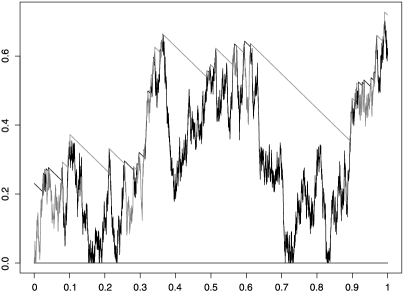
Figure 1: Simulated processes; Black $=X_{1}(\cdot)$, Gray $=X_{2}(\cdot)$.

5 Proof of Proposition 4.1

Given the planar Brownian motion $(V_{1}(\cdot),V_{2}(\cdot))$, we shall apply the idea of the proof of Theorem 1 of Harrison and Reiman [16] to study a system of equations for $(2A(\cdot),\sqrt{2}\Lambda(\cdot))^{\prime}$ equivalent to (54)–(55):

$$2A(t) = \max_{0\leq s\leq t}\bigl{(}{-|y|+\lambda s+\Lambda(s)-V^{\flat}(s)}\bigr{)}^{+},$$

$$\sqrt{2}\Lambda(t) = \max_{0\leq s\leq t}\bigl{(}{-\sqrt{2}r_{2}-\sqrt{2}gs+\sqrt{2}A(s)-\sqrt{2}\sigma V_{2}(s)}\bigr{)}^{+},$$

$$0\leq t<\infty,$$

with $V^{\mathbf{\flat}}(\cdot)=\rho V_{1}(\cdot)-\sigma V_{2}(\cdot)$ as in (33). Schematically, we shall write ${\mathbf{y}}(\cdot)=\bolds{\pi}_{\mathfrak{w}}({\mathbf{y}})(\cdot)$ for this system, with the two-dimensional Skorokhod map $\bolds{\pi}_{\mathfrak{w}}$ introduced in Harrison and Reiman [16]:

$$C_{0}\bigl{(}[0,\infty);\mathbb{R}^{2}\bigr{)}\ni{\mathbf{y}}(\cdot)\mapsto\bolds{\pi}_{\mathfrak{w}}({\mathbf{y}})(\cdot):=\sup_{0\leq s\leq\cdot}\bigl{[}{\mathbf{H}}{\mathbf{y}}(s)-{\mathfrak{w}}(s)\bigr{]}^{+}\in C_{0}\bigl{(}[0,\infty);\mathbb{R}^{2}\bigr{)}.$$ (96)

Here the subscript indicates the pinning ${\mathrm{y}}_{1}(0)={\mathrm{y}}_{2}(0)=0$; the matrix ${\mathbf{H}}$ is defined as

$${\mathbf{H}}=\frac{1}{\sqrt{2}}\pmatrix{0&1\cr 1&0},$$

and the component processes of the vector ${\mathfrak{w}}(\cdot)=({\mathfrak{w}}_{1}(\cdot),{\mathfrak{w}}_{2}(\cdot))^{\prime}$ are

$${\mathfrak{w}}_{1}(t) = |{y}|-\lambda t+V^{\flat}(t)=|{y}|-\lambda t+\rho V_{1}(t)-\sigma V_{2}(t),$$

$${\mathfrak{w}}_{2}(t) = \sqrt{2}r_{2}+\sqrt{2}gt+\sqrt{2}\sigma V_{2}(t),$$

$$0\leq t<\infty.$$

The supremum and the positive part $(\cdot)^{+}:=\max(\cdot,0)$ are taken for each element in the vectors.

The matrix ${\mathbf{H}}$ has spectral radius $1/\sqrt{2}$, so the mapping $\bolds{\pi}_{\mathfrak{w}}$ is a continuous, contraction mapping (Theorem 1 of Harrison and Reiman [16]); in particular, in terms of the sup-norm

$$\|{\mathbf{y}}\|_{T}:=\max_{1\leq i\leq 2}\sup_{0\leq s\leq T}\big{|}\mathrm{y}_{i}(s)\big{|}$$

for every ${\mathbf{y}},{\mathbf{y}}^{\flat}\in C_{0}([0,\infty);\mathbb{R}^{2})$ and $T\in[0,\infty)$ we have the bounds

$$\bigl{|}{\bolds{\pi}_{\mathfrak{w}}({\mathbf{y}})-\bolds{\pi}_{\mathfrak{w}}\bigl{(}{\mathbf{y}}^{\flat}\bigr{)}}\bigr{|}_{T}$$

$$\quad=\max\left[\sup_{0\leq s\leq T}\bigg{|}\sup_{0\leq u\leq s}\biggl{(}-{\mathfrak{w}}_{1}(s)+\frac{1}{\sqrt{2}}\mathrm{y}_{2}(s)\biggr{)}^{+}-\sup_{0\leq u\leq s}\biggl{(}-{\mathfrak{w}}_{1}(s)+\frac{1}{\sqrt{2}}\mathrm{y}_{2}^{\flat}(s)\biggr{)}^{+}\bigg{|},\right.$$

$$\hskip 46.0pt\left.\sup_{0\leq s\leq T}\bigg{|}\sup_{0\leq u\leq s}\biggl{(}-{\mathfrak{w}}_{2}(s)+\frac{1}{\sqrt{2}}\mathrm{y}_{1}(s)\biggr{)}^{+}-\sup_{0\leq u\leq s}\biggl{(}-{\mathfrak{w}}_{2}(s)+\frac{1}{\sqrt{2}}\mathrm{y}_{1}^{\flat}(s)\biggr{)}^{+}\bigg{|}\right]$$

$$\quad\leq\max\left[\sup_{0\leq s\leq T}\bigg{|}{-}\mathfrak{w}_{1}(s)+\frac{1}{\sqrt{2}}\mathrm{y}_{2}(s)-\biggl{(}-{\mathfrak{w}}_{1}(s)+\frac{1}{\sqrt{2}}\mathrm{y}_{2}^{\flat}(s)\biggr{)}\bigg{|},\right.$$

$$\hskip 46.0pt\left.\sup_{0\leq s\leq T}\bigg{|}{-}\mathfrak{w}_{2}(s)+\frac{1}{\sqrt{2}}\mathrm{y}_{1}(s)-\biggl{(}-{\mathfrak{w}}_{2}(s)+\frac{1}{\sqrt{2}}\mathrm{y}_{1}^{\flat}(s)\biggr{)}\bigg{|}\right]$$

$$\quad\leq\frac{1}{\sqrt{2}}\big{\|}{\mathbf{y}}-{\mathbf{y}}^{\flat}\big{\|}_{T}.$$

We have used here the contraction property of the maximum: for two continuous, real-valued functions $\mathrm{y}(\cdot),\mathrm{y}^{\flat}(\cdot)$ we have

$$\Bigl{|}{\sup_{0\leq s\leq T}\mathrm{y}(s)-\sup_{0\leq s\leq T}\mathrm{y}^{\flat}(s)}\Bigr{|} \leq \sup_{0\leq s\leq T}\bigl{|}{\mathrm{y}(s)-\mathrm{y}^{\flat}(s)}\bigr{|},\qquad 0\leq T<\infty,$$

$$\bigl{|}{\bigl{(}\mathrm{y}(s)\bigr{)}^{+}-\bigl{(}\mathrm{y}^{\flat}(s)\bigr{)}^{+}}\bigr{|} \leq \bigl{|}{\mathrm{y}(s)-\mathrm{y}^{\flat}(s)}\bigr{|},\qquad 0\leq s<\infty.$$

It follows from this contraction property that, given ${\mathfrak{w}}(\cdot)$, the solution ${\mathbf{y}}(\cdot)$ to the system of (5) can be obtained as the unique limit of a standard Picard–Lindelöf iteration: starting with ${\mathbf{y}}^{(1)}(\cdot)\equiv 0$, iterating ${\mathbf{y}}^{(n+1)}:=\bolds{\pi}_{\mathfrak{w}}({\mathbf{y}}^{(n)})$ for $n=1,2,\dots,$ we obtain the uniform convergence on compact intervals $\lim_{n\to\infty}\|{\mathbf{y}}-{\mathbf{y}}^{(n)}\|_{T}=0$ for $T\in(0,\infty)$. This concludes the proof of Proposition 4.1.

It might be interesting to investigate possible connections between this construction and the Skorokhod map on an interval, studied by Kruk et al. [24].

6 Proof of Propositions 4.2–4.4

Let us recall from (64), (62) that the process $(N(\cdot),M(\cdot))$ is a reflected planar Brownian motion in the $45$-degree wedge $\mathfrak{M}$ with orthogonal reflection on the faces:

$$N(t) = r_{1}-ht+\rho V_{1}(t)+A(t),\qquad 0\leq t<\infty,$$ (98)

$$M(t) = r_{2}+gt+\sigma V_{2}(t)-A(t)+\Lambda(t),\qquad 0\leq t<\infty.$$ (99)

This process does not hit the corner of the wedge $\mathfrak{M}$, if and only if it does not reach the corner during the time-horizon $[0,T]$ for any $T\in(0,\infty)$. Hence, in the nondegenerate case we can assume that the drift coefficients $g,h$ are equal to zero. Indeed, after a suitable change of probability measure on $\mathfrak{F}(T)$, under the new measure and on the finite time-horizon $[0,T]$ the process $(V_{1}(t)-(h/\rho)t,V_{2}(t)+(g/\sigma)t)_{t\in[0,T]}$ becomes then a two-dimensional standard Brownian motion, that is, a planar Brownian motion without drift.

Thus, in what follows we shall assume $h=g=0$ and apply the transformation $\mathfrak{T}=\operatorname{diag}(1/\rho,1/\sigma)$ to the process $(N(\cdot),M(\cdot))$ as in (98), (99). In matrix form, we can write

$$\mathfrak{T}\left[\matrix{N(t)\cr M(t)}\right]=\mathfrak{T}\left[\matrix{r_{1}\cr r_{2}}\right]+\left[\matrix{V_{1}(t)\cr V_{2}(t)}\right]+\mathfrak{T}\left[\matrix{1&0\cr-1&1}\right]\left[\matrix{A(t)\cr\Lambda(t)}\right];\qquad 0\leq t<\infty.$$ (100)

Then the transformed process is a reflected Brownian motion in the wedge $\mathfrak{W}=\mathfrak{T}(\mathfrak{M})$ with oblique reflection on the faces.

We need to compute the angle $\bolds{\xi}$ of the wedge $\mathfrak{W}$ at the corner, and also the reflection angles $\bolds{\theta}_{i}\in(-\uppi/2,\uppi/2)$ $i=1,2$ measured from the inward normal vector on the boundary, and positive if and only if they direct the process toward the corner; see Figure 2 below. We introduce also the scalar parameter

$$\bolds{\alpha}:=(\bolds{\theta}_{1}+\bolds{\theta}_{2})/\bolds{\xi}.$$ (101)

According to Theorems 2.2 and 3.10 of Varadhan and Williams [33], the reflected Brownian motion in the wedge $\mathfrak{W}$ never hits the corner of the wedge $\mathfrak{W}$, with probability one, if $\bolds{\alpha}\leq 0$; hits the corner with probability one, if $\bolds{\alpha}>0$; and is well-defined by the corresponding submartingale problem for all times, starting at any initial point including the corner, if $\bolds{\alpha}<2$.

Now the faces of the wedge $\mathfrak{W}$ are given by half-lines emanating from the origin and parallel to the vectors $\mathfrak{v}_{1}=\mathfrak{T}(1,0)^{\prime}=(1/\rho,0)^{\prime}$ and $\mathfrak{v}_{2}=\mathfrak{T}(1,1)^{\prime}=(1/\rho,1/\sigma)^{\prime}$, hence

$$\cos(\bolds{\xi})=\frac{\langle{\mathfrak{v}_{1}},{\mathfrak{v}_{2}}\rangle}{\|{\mathfrak{v}_{1}}\|\|{\mathfrak{v}_{2}}\|}=\frac{\rho^{-2}}{\sqrt{\rho^{-2}+\sigma^{-2}}\sqrt{\rho^{-2}}}=\sigma.$$ (102)

The reflection vector on the face of the wedge $\mathfrak{W}$ parallel to $\mathfrak{v}_{2}=(1/\rho,1/\sigma)^{\prime}$ is $\bolds{\nu}_{2}:=(1/\rho,-1/\sigma)^{\prime}$, while the normal vector of this face pointing inward is $\mathbf{n}_{2}=(\rho,-\sigma)^{\prime}$. Then

$$\bolds{\nu}_{2}-\frac{\langle{\bolds{\nu}_{2}},{\mathbf{n}_{2}}\rangle}{\|{\mathbf{n}_{2}}\|^{2}}\mathbf{n}_{2}=\bolds{\nu}_{2}-2\mathbf{n}_{2}=(1/\rho-2\rho,2\sigma-1/\sigma)^{\prime}=\bigl{(}\sigma^{2}-\rho^{2}\bigr{)}\cdot(1/\rho,1/\sigma)^{\prime},$$

so $\bolds{\nu}_{2}$ points towards to the corner exactly when $\sigma^{2}<\rho^{2}$. That is, $\bolds{\theta}_{2}>0$ holds if and only if $\sigma^{2}<1/2$.

The other face of the wedge $\mathfrak{W}$ is parallel to $(1,0)^{\prime}$ and the reflection vector on this face is $(0,1/\sigma)^{\prime}$, which is a normal vector to this face, whence $\bolds{\theta}_{1}=0$.

Proof of Proposition 4.2 If $1>\sigma^{2}\geq 1/2$, then

$$\bolds{\theta}_{1}=0,\qquad\bolds{\theta}_{2}\leq 0,\qquad\bolds{\xi}>0,$$ (103)

so $\bolds{\alpha}\leq 0$. Thus, according to the result of Harrison and Reiman [16] and Varadhan and Williams [33], with probability one the process $(N(\cdot),M(\cdot))$ never hits the corner of the wedge $\mathfrak{M}$. The case $\sigma^{2}=1$ is discussed in Section 6.1.

Proof of Proposition 4.3 In the case $0<\sigma^{2}<1/2$, we obtain $\cos(\bolds{\xi})<1/\sqrt{2}$ from (102) and

$$\bolds{\theta}_{1}=0,\qquad 0<\bolds{\theta}_{2}<\uppi/2,\qquad\bolds{\xi}>\uppi/4,$$

so $0<\bolds{\alpha}<2$. Then the process $(N(\cdot),M(\cdot))$ hits the corner of the wedge $\mathfrak{M}$ almost surely. This gives the result for $g=h=0$.

When $g+h>0$, we can only ascertain that the process $(N(\cdot),M(\cdot))$ hits the corner of the wedge with positive probability, due to the measure change step that we deployed to reduce the general case to the driftless case.

6.1 Nonattainability of the corner in the degenerate case $\rho=0$

In this subsection, we develop the proof of Proposition 4.2 in the degenerate case $\sigma=1,\rho=0$. The equations of (98), (99) for the ranked processes $N(\cdot)\geq M(\cdot)\geq 0$ simplify then to

$$N(t) = r_{1}-ht+A(t),\qquad 0\leq t<\infty,$$ (104)

$$M(t) = r_{2}+gt+V(t)-A(t)+\Lambda(t),\qquad 0\leq t<\infty;$$ (105)

we recall that the “regulating” continuous, increasing and adapted processes $A(\cdot),\Lambda(\cdot)$ of (54), (55) satisfy the $\mathbb{P}$-a.e. requirements

$$\int_{0}^{\infty}\mathbf{1}_{\{N(t)>M(t)\}}\,\mathrm{d}A(t)=0,\qquad\int_{0}^{\infty}\mathbf{1}_{\{M(t)>0\}}\,\mathrm{d}\Lambda(t)=0$$ (106)

as in (60), (63). We introduce the stopping time $\tau=\inf\{{t>0\colon\ N(t)=0}\}$, and shall establish below the property $\mathbb{P}(\tau=\infty)=1$.

For this, it suffices to consider $h>0$; for if $h=0$, the process $N(\cdot)$ is nondecreasing, and there is nothing to prove. Whereas, by the Girsanov theorem, it is enough to deal with the case $g=0$. We shall present two distinct, very different arguments.

$\bullet$ First argument: In the manner of Section 4.2, we consider the unfolded process $(N(\cdot),$ $M^{\dagger}(\cdot))$, where $M(\cdot)=|{M^{\dagger}(\cdot)}|$ and $\mathrm{d}M^{\dagger}(t)=\overline{\operatorname{sgn}}(M^{\dagger}(t))\,\mathrm{d}M(t)$, stopped upon reaching the corner:

$$N(t)=r_{1}-ht+A(t),\qquad M^{\dagger}(t)=r_{2}+V^{\dagger}(t)-\int_{0}^{t}\overline{\operatorname{sgn}}\bigl{(}M^{\dagger}(s)\bigr{)}\,\mathrm{d}A(s)$$

for $0\leq t\leq\tau$; and $M(t)=N(t)=0$ for $t\geq\tau$. Here $V^{\dagger}(\cdot):=\int_{0}^{\cdot}\overline{\operatorname{sgn}}(M^{\dagger}(s))\,\mathrm{d}V(s)=\int_{0}^{\cdot}\operatorname{sgn}(M^{\dagger}(s))\,\mathrm{d}V(s)$ is of course standard Brownian motion; the equality of the two stochastic integrals follows by applying the second property of (2) to the semimartingale $M(\cdot)$ of (105).

The planar process $(N(\cdot),M^{\dagger}(\cdot))$ evolves in the cone $\{{(x,y)\colon\ 0\leq|{y}|\leq x}\}$, with normal reflection on the faces and absorption when the corner of the cone is reached. It is clear that $(N(\cdot),M^{\dagger}(\cdot))$ is a strong Markov process; when started at $(x,y)$, the distribution of this process will be denoted by $\mathbb{P}_{(x,y)}$. We shall show that $\mathbb{P}(\tau=\infty)=1$.

For this purpose, we define a Markov chain $\{(\widetilde{S}_{n},Y_{n})\}_{n\geq 0}$ with

$$\widetilde{S}_{n}:=\log_{(2)}\bigl{(}N(\tau_{n})/r_{1}\bigr{)},\qquad Y_{n}:=M^{\dagger}(\tau_{n})/N(\tau_{n}),$$

where we have set $\tau_{0}:=0$ and recursively $\tau_{n+1}:=\inf\{{t>\tau_{n}\colon\ (N(t)/N(\tau_{n}))\notin[1/2,2]}\}$, and noted that $\tau_{n}$ is a.s. finite, for all $n\in\mathbb{N}_{0}$. The state-space of this Markov chain is $\mathbb{Z}\times[-1,1]$. For $k>0$, we shall denote

$$\widetilde{\rho}_{k}:=\inf\{n\in\mathbb{N}_{0}\colon\ \widetilde{S}_{n}=\widetilde{S}_{0}+k\}.$$

A simple sufficient condition for the nonattainability of the origin by $N(\cdot)$ is that

$$\widetilde{\rho}_{k} k>0$$ is finite almost surely for all . (107)

Indeed, on $\{{\tau<\infty}\}$ the sample path of the process $N(\cdot)$ is bounded, because it is continuous. It is clear from this that $\{{\tau<\infty}\}\subset\bigcup_{k}\{{\widetilde{\rho}_{k}=\infty}\}$, and $\mathbb{P}(\tau<\infty)=0$ follows from (107).

We compare $\widetilde{\mathbf{S}}=\{\widetilde{S}_{n}\}_{n\geq 0}$ with a random walk $\mathbf{S}=\{S_{n}\}_{n\geq 0}$ on $\mathbb{Z}$, which starts at $S_{0}=0$ and is defined by

$$\mathbb{P}({S_{n+1}=S_{n}+1\mid S_{0},\dots,S_{n}})=\mathfrak{p}\bigl{(}r_{1}2^{S_{n}}\bigr{)},\qquad\mathbb{P}({S_{n+1}=S_{n}-1\mid S_{0},\dots,S_{n}})=1-\mathfrak{p}\bigl{(}r_{1}2^{S_{n}}\bigr{)}$$

as its transition probabilities, where

$$\mathfrak{p}(r):=\inf_{y\in[-r,r]}\mathbb{P}_{(r,y)}\bigl{(}{N(\tau_{1})=2r}\bigr{)}.$$

To wit: we start the process $(N(\cdot),M^{\dagger}(\cdot))$ from a point on the vertical line at $x=r$, and denote by $\mathfrak{p}(r)$ the greatest lower bound on the probability that $N(\cdot)$ hits $2r$ before it hits $r/2$. We prove below that

$$\lim_{r\to 0+}\mathfrak{p}(r)=1\quad\mbox{and}\quad\mathfrak{p}(r)>0\qquad\mbox{for all $r>0$}.$$ (108)

On a suitable extension of our probability space there is a coupling between $\widetilde{\mathbf{S}}$ and the random walk $\mathbf{S}$, such that $\widetilde{S}_{n}\geq S_{n}$, $\forall n\in\mathbb{N}_{0}$. Therefore, the sufficient condition (107) will be established as soon as we show that $\rho_{k}=\inf\{{n\geq 0\colon\ S_{n}=k}\}\geq\tilde{\rho}_{k}$ is a.s. finite, for all $k>0$.

Let $\ell_{0}\leq 0$ be such that $\mathfrak{p}(r_{1}2^{\ell})\geq 1/2$ holds for $\ell\leq\ell_{0}$, and consider a simple, symmetric random walk $\widehat{\mathbf{S}}=\{\widehat{S}_{n}\}_{n\geq 0}$ on the state space $\{{\ell\colon\ \ell\leq\ell_{0}}\}$, with $\ell_{0}$ as both reflecting barrier and starting point. Using coupling again, we can assume that $\widehat{S}_{n}\leq S_{n}$ holds for all $n\in\mathbb{N}_{0}$. Fix $k>0$ and recall that $\widehat{\mathbf{S}}$ is recurrent. Thus, if $\mathbf{S}$ does not reach $k$ before reaching $\ell_{0}-1$, it will return to the level $\ell_{0}$ almost surely; and from $\ell_{0}$ it will reach $k$ before reaching $\ell_{0}-1$, with some positive probability. If, on the other hand, $\mathbf{S}$ hits $\ell_{0}-1$ first, then the whole thing starts again and finally $k$ is reached almost surely by $\mathbf{S}$. By a standard renewal argument, this implies that $\mathbf{S}$ reaches $S_{0}+k$ almost surely, and that $\rho_{k}=\inf\{{n\geq 0\colon\ S_{n}=S_{0}+k}\}$ is finite almost surely.

It remains now only to argue (108). Let $r>0$ and observe that, if $N(0)=r$ and $|{M^{\dagger}(0)}|\leq r$, then $N(\tau_{1})=r/2$ implies that $\tau_{1}\geq(r/2h)$ and $|{V^{\dagger}(r/2h)}|<4r$, hence

$$1-\mathfrak{p}(r)=\sup_{y\in[-r,r]}\mathbb{P}_{(r,y)}\bigl{(}N(\tau_{1})=r/2\bigr{)}\leq\mathbb{P}\bigg{(}\biggl{|}{V^{\dagger}\biggl{(}{\frac{r}{2h}}\biggr{)}}\biggr{|}<4r\bigg{)},$$

that is,

$$\mathfrak{p}(r)\geq 1-\mathbb{P}\bigg{(}{\biggl{|}{V^{\dagger}\biggl{(}{\frac{r}{2h}}\biggr{)}}\biggr{|}<4r}\bigg{)}=\mathbb{P}\bigg{(}{\bigl{|}{V^{\dagger}(1)}\bigr{|}>4\sqrt{2hr}}\bigg{)}.$$

This justifies (108) and completes the proof of the nonattainability of the corner in the degenerate case, thus also the proof of Proposition 4.2.

$\bullet$ Second argument: Here follows another argument, due to Dr.E.Robert Fernholz; we shall take $r_{2}=0$ for simplicity. With $B(\cdot)$ a standard Brownian motion, we denote by $\Gamma(\cdot)$ the Skorokhod reflection of the process $r_{1}-ht-B(t),0\leq t<\infty$, and by $\Delta(\cdot)$ the Skorokhod reflection of $r_{1}-ht+B(t),0\leq t<\infty$:

$$\Gamma(t)=r_{1}-ht-B(t)+L^{\Gamma}(t)\geq 0,\qquad\Delta(t)=r_{1}-ht+B(t)+L^{\Delta}(t)\geq 0,$$ (109)

where the continuous, increasing processes

$$L^{\Gamma}(t):=\max_{0\leq s\leq t}\bigl{(}hs+B(s)-r_{1}\bigr{)}^{+},\qquad L^{\Delta}(t):=\max_{0\leq s\leq t}\bigl{(}hs-B(s)-r_{1}\bigr{)}^{+}$$

satisfy the $\mathbb{P}$-a.s. identities $\int_{0}^{\infty}\mathbf{1}_{\{\Gamma(t)>0\}}\,\mathrm{d}L^{\Gamma}(t)=0$, $\int_{0}^{\infty}\mathbf{1}_{\{\Delta(t)>0\}}\,\mathrm{d}L^{\Delta}(t)=0$. We define

$$Y_{2}(t) := B(t)-{\textstyle\frac{1}{2}}L^{\Gamma}(t)+{\textstyle\frac{1}{2}}L^{\Delta}(t),\qquad Y_{1}(t):=Y_{2}(t)+\Gamma(t),$$

$$Y_{3}(t) := Y_{2}(t)-\Delta(t),$$

and note

$$Y_{1}(t)=-Y_{3}(t)=r_{1}-ht+{\textstyle\frac{1}{2}}\bigl{(}L^{\Gamma}(t)+L^{\Delta}(t)\bigr{)}\geq\bigl{|}{Y_{2}(t)}\bigr{|},\qquad 0\leq t<\infty.$$ (111)

We shall show below that, with probability one,

$$\mbox{{the three-dimensional process} }\bigl{(}Y_{1}(\cdot),Y_{2}(\cdot),Y_{3}(\cdot)\bigr{)}\mbox{ {exhibits no triple point}}.$$ (112)

Then the comparisons in (111) imply

$$\mathbb{P}\bigl{(}Y_{1}(t)>0,\forall t\in[0,\infty)\bigr{)}=1.$$ (113)

To prove (112), it suffices to rule out triple points for the process $(\widehat{Y}_{1}(\cdot),\widehat{Y}_{2}(\cdot),\widehat{Y}_{3}(\cdot))$ with components $\widehat{Y}_{j}(\cdot):=Y_{j}(\cdot)+(L^{\Gamma}(\cdot)-L^{\Delta}(\cdot))/2$, $j=1,2,3,$ namely

$$\widehat{Y}_{1}(t)=r_{1}-ht+L^{\Gamma}(t)\geq\widehat{Y}_{2}(t)=B(t)\geq\widehat{Y}_{3}(t)=-r_{1}+ht-L^{\Delta}(t),\qquad 0\leq t<\infty.$$

Consider the set $E$ of all $\omega\in\Omega$ for which $\widehat{Y}_{1}(T)=\widehat{Y}_{2}(T)=\widehat{Y}_{3}(T)=:y$ holds for some $T=T(\omega)\in(0,\infty)$. Then, for each $t\in[0,T)$ we have

$$y+h(T-t) \geq y+h(T-t)-L^{\Gamma}(T)+L^{\Gamma}(t)=\widehat{Y}_{1}(t)\geq\widehat{Y}_{2}(t)=y+B(T)-B(t)$$

$$\geq \widehat{Y}_{3}(t)=y-h(T-t)+L^{\Delta}(T)-L^{\Delta}(t)\geq y-h(T-t)$$

thus also

$$-h\leq{B(T)-B(t)\over T-t}\leq h.$$

In conjunction with the Paley, Wiener and Zygmund theorem (cf. page 110 in Karatzas and Shreve [23]), we conclude that $E$ is included in an event of $\mathbb{P}$-measure zero, so (112) follows. (We are indebted to Dr. Johannes Ruf, for pointing out the relevance of the Paley–Wiener–Zygmund theorem here.)

Let us define now

$$Q_{1}(\cdot):=Y_{1}(\cdot),\qquad Q_{2}(\cdot):=\big{|}Y_{2}(\cdot)\big{|}$$ (114)

and apply the companion Tanaka formula (18) to get $Q_{2}(\cdot)=\int_{0}^{\cdot}\overline{\operatorname{sgn}}(Y_{2}(t))\,\mathrm{d}Y_{2}(t)+L^{Q_{2}}(\cdot)$. In conjunction with (6.1), the fact that $L^{\Gamma}(\cdot)=L^{Y_{1}-Y_{2}}(\cdot)$ is flat off the set $\{t\geq 0\colon\ Y_{2}(t)=Y_{1}(t)>0\}$, and the fact that $L^{\Delta}(\cdot)=L^{Y_{2}-Y_{3}}(\cdot)$ is flat off the set $\{t\geq 0\colon\ Y_{2}(t)=Y_{3}(t)<0\}$, this leads to

$$Q_{2}(\cdot)=\widehat{V}(\cdot)-{\textstyle\frac{1}{2}}\bigl{(}L^{Y_{1}-Y_{2}}(\cdot)+L^{Y_{1}+Y_{2}}(\cdot)\bigr{)}+L^{Q_{2}}(\cdot),$$ (115)

where

$$\widehat{V}(\cdot):=\int_{0}^{\cdot}\overline{\operatorname{sgn}}\bigl{(}Y_{2}(t)\bigr{)}\,\mathrm{d}B(t)=\int_{0}^{\cdot}\operatorname{sgn}\bigl{(}Y_{2}(t)\bigr{)}\,\mathrm{d}B(t)$$

is standard Brownian motion (for this last equality, we have applied the second property of (2) to the semimartingale $Y_{2}(\cdot)$ in (6.1)). From (114), (6.1) and (111), we have then

$$Q_{1}(\cdot) = r_{1}-ht+{\textstyle\frac{1}{2}}\bigl{(}L^{Y_{1}-Y_{2}}(\cdot)+L^{Y_{1}+Y_{2}}(\cdot)\bigr{)},$$ (116)

$$0 \leq Q_{1}(\cdot)-Q_{2}(\cdot)=r_{1}-ht-\widehat{V}(\cdot)-L^{Q_{2}}(\cdot)+\bigl{(}L^{Y_{1}-Y_{2}}(\cdot)+L^{Y_{1}+Y_{2}}(\cdot)\bigr{)}.$$ (117)

But the continuous, increasing process $L^{Y_{1}-Y_{2}}(\cdot)+L^{Y_{1}+Y_{2}}(\cdot)$ is flat away from the set $\{Q_{1}(\cdot)=Q_{2}(\cdot)\}=\{Y_{1}(\cdot)\pm Y_{2}(\cdot)=0\}$, so the theory of the Skorokhod reflection problem gives the $\mathbb{P}$-a.e. identities

$$L^{Y_{1}-Y_{2}}(\cdot)+L^{Y_{1}+Y_{2}}(\cdot)\equiv L^{Q_{1}-Q_{2}}(\cdot),\qquad\int_{0}^{\infty}\mathbf{1}_{\{Q_{1}(t)>Q_{2}(t)\}}\,\mathrm{d}L^{Q_{1}-Q_{2}}(t)=0.$$

With this identification, the system (117), (116) is written equivalently as

$$Q_{1}(t) = r_{1}-ht+{\textstyle\frac{1}{2}}L^{Q_{1}-Q_{2}}(t),$$ (118)

$$Q_{2}(t) = \widehat{V}(t)-{\textstyle\frac{1}{2}}L^{Q_{1}-Q_{2}}(t)+L^{Q_{2}}(t)$$ (119)

with $\int_{0}^{\infty}\mathbf{1}_{\{Q_{2}(t)>0\}}\,\mathrm{d}L^{Q_{2}}(t)=0$, $\int_{0}^{\infty}\mathbf{1}_{\{Q_{1}(t)>Q_{2}(t)\}}\,\mathrm{d}L^{Q_{1}-Q_{2}}(t)=0$; that is, precisely in the form (104)–(106) with $g=0$, $r_{2}=0$. Thus, the pairs $(Q_{1}(\cdot),Q_{2}(\cdot))$ and $(N(\cdot),M(\cdot))$ have the same distribution, so the property $\mathbb{P}(N(t)>0,\forall t\in[0,\infty))=1$ follows now from (113) and (114).

6.2 Proof of Proposition 4.4

In the nondegenerate case $\sigma^{2}<1$, the properties of (68) follow from Theorem 1 in Reiman and Williams [31]; see also Theorem 7.7 in Bhardwaj and Williams [3]. In the degenerate case $\sigma^{2}=1$, they follow from (60), (63) – which give $A(\cdot)=\int_{0}^{\cdot}\mathbf{1}_{\{G(t)=0\}}\,\mathrm{d}A(t)$ and $\Lambda(\cdot)=\int_{0}^{\cdot}\mathbf{1}_{\{M(t)=0\}}\,\mathrm{d}\Lambda(t)$, respectively – and the nonattainability of the corner that we just proved.

7 Questions of uniqueness

Let $\mathcal{B}(\cdot)=(B_{1}(\cdot),B_{2}(\cdot))^{\prime}$ be a planar Brownian motion, and define the matrix- and vector-valued functions $\bolds{\Sigma}\mathchoice{\nobreak\,\colon}{\nobreak\,\colon}{\nobreak\,\colon\;}{\nobreak\,\colon\;}\mathbb{R}^{2}\to\mathbb{R}^{2\times 2}$ and $\bolds{\mu}\mathchoice{\nobreak\,\colon}{\nobreak\,\colon}{\nobreak\,\colon\;}{\nobreak\,\colon\;}\mathbb{R}^{2}\to\mathbb{R}^{2}$ by

$$\bolds{\Sigma}(x) = \mathbf{1}_{\{x_{1}>x_{2}\}}\operatorname{diag}(\rho,\sigma)+\mathbf{1}_{\{x_{1}\leq x_{2}\}}\operatorname{diag}(\sigma,\rho),$$

$$\bolds{\mu}(x) = \mathbf{1}_{\{x_{1}>x_{2}\}}(-h,g)^{\prime}+\mathbf{1}_{\{x_{1}\leq x_{2}\}}(g,-h)^{\prime}$$

for $x=(x_{1},x_{2})\in\mathbb{R}^{2}$. We are interested in questions of uniqueness for the system of stochastic differential equations (2.2) and (2.2), written now a bit more conveniently in the vector form

$$\mathrm{d}\mathcal{X}(t)=\bolds{\mu}\bigl{(}\mathcal{X}(t)\bigr{)}\,\mathrm{d}t+\bolds{\Sigma}\bigl{(}\mathcal{X}(t)\bigr{)}\,\mathrm{d}\mathcal{B}(t)+\mathrm{d}\mathcal{L}^{\mathcal{X}}(t).$$ (120)

Here we have denoted the vector of semimartingale local time processes accumulated at the origin by the components of the planar process $\mathcal{X}(\cdot)=(X_{1}(\cdot),X_{2}(\cdot))^{\prime}$ as

$$\mathcal{L}^{\mathcal{X}}(\cdot):=\bigl{(}L^{X_{1}}(\cdot),L^{X_{2}}(\cdot)\bigr{)}^{\prime};$$ (121)

these local times are responsible for keeping the planar process $\mathcal{X}(\cdot)$ in the nonnegative quadrant.

7.1 Pathwise uniqueness

For any given initial condition $\mathcal{X}(0)$ in the punctured nonnegative quadrant of (7), we have shown that the stochastic differential equation (120) has a solution. We want to show that this solution is pathwise unique, up to the first hitting time of the corner of the quadrant. Under the condition (6), the origin is never hit by the process $\mathcal{X}(\cdot)$, so pathwise uniqueness will hold then for all times. The key step is to define the new planar process

$$\mathcal{Z}(\cdot)=\bigl{(}Z_{1}(\cdot),Z_{2}(\cdot)\bigr{)}^{\prime}\qquad\mbox{with }Z_{i}(\cdot):=X_{i}(\cdot)-L^{X_{i}}(\cdot)\qquad(i=1,2),$$ (122)

and note, from the Skorokhod reflection problem once again, that

$$L^{X_{i}}(t)=Z^{*}_{i}(t):=\max_{0\leq s\leq t}\bigl{(}-Z_{i}(s)\bigr{)}\vee 0,\qquad 0\leq t<\infty.$$ (123)

(In particular, each $X_{i}(\cdot)$, $i=1,2$ is the Skorokhod reflection of the semimartingale $Z_{i}(\cdot)$ in (122).) We observe that $\mathcal{X}(\cdot)$ solves the equation (120), if and only if $\mathcal{Z}(\cdot)$ solves the stochastic differential equation with path-dependent coefficients

$$\mathrm{d}\mathcal{Z}(t)=\bolds{\mu}\bigl{(}\mathcal{Z}(t)+\mathcal{Z}^{*}(t)\bigr{)}\,\mathrm{d}t+\bolds{\Sigma}\bigl{(}\mathcal{Z}(t)+\mathcal{Z}^{*}(t)\bigr{)}\,\mathrm{d}\mathcal{B}(t),\qquad\mathcal{Z}(0)=\mathcal{X}(0)\in\mathfrak{S},$$ (124)

where, with the notation of (123), we have set

$$\mathcal{Z}^{*}(t):=\bigl{(}Z_{1}^{*}(t),Z_{2}^{*}(t)\bigr{)}^{\prime}=\Bigl{(}\max_{0\leq s\leq t}\bigl{(}-Z_{1}(t)\bigr{)}\vee 0,\max_{0\leq s\leq t}\bigl{(}-Z_{2}(t)\bigr{)}\vee 0\Bigr{)}^{\prime}.$$ (125)

Indeed, if $(\mathcal{X}(\cdot),\mathcal{B}(\cdot))$ is a solution of (120) with the vector process $L^{\mathcal{X}}(\cdot)$ given as in (121), and if we define $\mathcal{Z}(\cdot)$ in accordance with (122), then $(\mathcal{Z}(\cdot),\mathcal{B}(\cdot))$ is a solution of (124). And conversely, if $(\mathcal{Z}(\cdot),\mathcal{B}(\cdot))$ is a solution of (124) and we define

$$\mathcal{X}(\cdot):=\mathcal{Z}(\cdot)+\mathcal{Z}^{*}(\cdot)$$ (126)

in the notation of (125), we identify $\mathcal{Z}^{*}(\cdot)$ as the coordinate-wise local time of $\mathcal{X}(\cdot)$, namely $\mathcal{Z}^{*}(\cdot)=\mathcal{L}^{\mathcal{X}}(\cdot)$ as in (121). In particular, pathwise uniqueness for the equation (124) with path-dependent coefficients, implies pathwise uniqueness for the equation (120) with local times.

For the equation (124), this pathwise uniqueness result can be seen by exploiting the fact that the only critical time-points occur when the process $\mathcal{X}(\cdot)$ of (126) hits either the boundary of the quadrant, or its diagonal. Thus, we set $\tau_{0}:=0$, and introduce inductively the stopping times

$$\tau_{2n+1} := \inf\bigl{\{}t>\tau_{2n}\colon\ \bigl{(}Z_{1}(t)+Z^{*}_{1}(t)\bigr{)}\bigl{(}Z_{2}(t)+Z^{*}_{2}(t)\bigr{)}=0\bigr{\}},$$

$$\tau_{2n+2} := \inf\bigl{\{}t>\tau_{2n+1}\colon\ Z_{1}(t)+Z^{*}_{1}(t)=Z_{2}(t)+Z^{*}_{2}(t)\bigr{\}}$$

for $n\in\mathbb{N}_{0}$. It might happen that $\tau_{1}=\tau_{0}=0$ holds with positive probability, if $\mathcal{X}(0)=\mathcal{Z}(0)$ is on one of the faces of the quadrant. Apart from that, we have $\tau_{k+1}>\tau_{k}$ for all $k\geq 1$; and with $\tau:=\sup_{k\in\mathbb{N}}\tau_{k}$, we observe that $\mathcal{X}(\tau)=\mathcal{Z}(\tau)+\mathcal{Z}^{*}(\tau)$ lies on one of the faces of the quadrant and also on its diagonal, hence $\mathcal{X}(\tau)=(0,0)$. Whereas, under the condition (6), we know that $\mathcal{X}(\cdot)$ never reaches the corner of the quadrant, so $\tau$ is almost surely infinite. Then pathwise uniqueness up to $\tau$ can be established by induction; namely, by showing that on each time-interval $[\tau_{k-1},\tau_{k}]$ with $k\geq 1$ the process $\mathcal{Z}(\cdot)$ solves an equation with pathwise unique solution.

Assume first that $k-1$ is odd; then on the time-interval $[\tau_{k-1},\tau_{k}]$ the drift and diffusion coefficients are constant, so pathwise uniqueness follows immediately. If $k-1$ is even, then $\mathcal{Z}^{*}(\cdot)$ is constant on the interval $[\tau_{k-1},\tau_{k}]$, and the process $\mathcal{X}(\cdot)=\mathcal{Z}(\cdot)+\mathcal{Z}^{*}(\cdot)$ solves on $[\tau_{k-1},\tau_{k}]$ the equation studied in Fernholz et al. [13], Theorem 5.1, where it was shown that the solution of this equation is pathwise unique. This completes the induction argument.

Invoking the Yamada–Watanabe theory (e.g., Karatzas and Shreve [23], pages 308–311), we obtain from all this the following result.

Proposition 7.1

For the system of equations (2.2) and (2.2), pathwise uniqueness holds up until the first hitting time $\tau$ of (8).

Under the condition $1/2\leq\sigma^{2}<1$ of (6) pathwise uniqueness, thus also uniqueness in distribution, hold for all times, so the solution of (2.2) and (2.2) is then strong; that is, for all $0\leq t<\infty$ we have

$$\mathfrak{F}^{(X_{1},X_{2})}(t)\subseteq\mathfrak{F}^{(B_{1},B_{2})}(t).$$ (127)

This completes the proof of Theorems 1.1 and 1.3. It is an open question to settle, whether such pathwise uniqueness and strength hold also past the first hitting time of the corner, or not.

7.2 Uniqueness in distribution

This section will be devoted to the proof of Theorem 1.2 on uniqueness in distribution. In the light of Proposition 7.1 and Theorem 1.3, this needs elaboration only when $0<\sigma^{2}<1/2$ as in (67). In this case, the state process $\mathcal{X}(\cdot)=(X_{1}(\cdot),X_{2}(\cdot))^{\prime}$ of (120) can reach the corner of the quadrant $[0,\infty)^{2}$ in finite time, and the question is whether it can be continued beyond that time in a well-defined and unique-in-distribution manner.

Proof of Theorem 1.2 It is quite straightforward to see that the weak solution construction of Section 4, culminating with the continuous, nonnegative processes $X_{1}(\cdot),X_{2}(\cdot)$ defined in Section 4.4, makes perfectly good sense also for an initial condition $(X_{1}(0),X_{2}(0))=(x_{1},x_{2})=(0,0)$ at the corner of the quadrant. Together with the independent Brownian motions $B_{1}(\cdot),B_{2}(\cdot)$ of (72), (73), these processes $X_{1}(\cdot),X_{2}(\cdot)$ are constituents of a weak solution for the system (120), and from (121)–(123) we have the representations

$$X_{i}(\cdot)=Z_{i}(\cdot)+\max_{0\leq s\leq\cdot}\bigl{(}-Z_{i}(s)\bigr{)},\qquad i=1,2.$$

Now, on an extension of the filtered probability space on which $(B_{1}(\cdot),B_{2}(\cdot))$ is still planar Brownian motion, we unfold these continuous, nonnegative semimartingales as

$$X_{i}(\cdot)=\big{|}Z_{i}^{\flat}(\cdot)\big{|},\qquad\mbox{where }Z_{i}^{\flat}(\cdot)=\int^{\cdot}_{0}\overline{\operatorname{sgn}}\bigl{(}Z_{i}^{\flat}(s)\bigr{)}\,\mathrm{d}Z_{i}(s).$$

This is done using the Prokaj [29] construction of Section 4.2 once again. It follows that the process $\mathcal{Z}^{\flat}(\cdot):=(Z_{1}^{\flat}(\cdot),Z_{2}^{\flat}(\cdot))^{\prime}$ with component-wise absolute values $|\mathcal{Z}^{\flat}(\cdot)|:=(|Z_{1}^{\flat}(\cdot)|,|Z_{2}^{\flat}(\cdot)|)^{\prime}$ $=\mathcal{X}(\cdot)$ satisfies the vector stochastic differential equation

$$\mathrm{d}\mathcal{Z}^{\flat}(\cdot) = \mathbf{I}\bigl{(}\mathcal{Z}^{\flat}(t)\bigr{)}\bigl{(}\bolds{\mu}\bigl{(}\mathcal{X}(t)\bigr{)}\,\mathrm{d}t+\bolds{\Sigma}\bigl{(}\mathcal{X}(t)\bigr{)}\,\mathrm{d}\mathcal{B}(t)\bigr{)}$$

$$= \mathbf{I}\bigl{(}\mathcal{Z}^{\flat}(t)\bigr{)}\bolds{\mu}\bigl{(}\big{|}\mathcal{Z}^{\flat}(t)\big{|}\bigr{)}\,\mathrm{d}t+\mathbf{I}\bigl{(}\mathcal{Z}^{\flat}(t)\bigr{)}\bolds{\Sigma}\bigl{(}\big{|}\mathcal{Z}^{\flat}(t)\big{|}\bigr{)}\,\mathrm{d}\mathcal{B}(t),\qquad 0\leq t<\infty,$$

with the initial condition $\mathcal{Z}^{\flat}(0)=0$, the indicator matrix function

$$\mathbf{I}(z):=\operatorname{diag}\bigl{(}\overline{\operatorname{sgn}}(z_{1}),\overline{\operatorname{sgn}}(z_{2})\bigr{)}\qquad\mbox{and the notation }z=(z_{1},z_{2})^{\prime}\in\mathbb{R}^{2},|z|:=\bigl{(}|z_{1}|,|z_{2}|\bigr{)}^{\prime}.$$

The functions $\mathbf{I}(\cdot)\bolds{\mu}(|\cdot|)$ and $\mathbf{I}(\cdot)\bolds{\Sigma}(|\cdot|)$ are piecewise constant in the interior of each one of the eight wedges

$$\bigl{\{}(z_{1},z_{2})\colon\ z_{1}\geq 0,z_{2}\geq 0,z_{1}>z_{2}\bigr{\}},\qquad\bigl{\{}(z_{1},z_{2})\colon\ z_{1}\geq 0,z_{2}\geq 0,z_{1}\leq z_{2}\bigr{\}},$$

$$\bigl{\{}(z_{1},z_{2})\colon\ z_{1}<0,z_{2}\geq 0,z_{1}\geq z_{2}\bigr{\}},\qquad\bigl{\{}(z_{1},z_{2})\colon\ z_{1}<0,z_{2}\geq 0,z_{1}\leq z_{2}\bigr{\}},$$

$$\bigl{\{}(z_{1},z_{2})\colon\ z_{1}\geq 0,z_{2}<0,z_{1}>z_{2}\bigr{\}},\qquad\bigl{\{}(z_{1},z_{2})\colon\ z_{1}\geq 0,z_{2}<0,z_{1}\leq z_{2}\bigr{\}},$$

$$\bigl{\{}(z_{1},z_{2})\colon\ z_{1}<0,z_{2}<0,z_{1}>z_{2}\bigr{\}},\qquad\bigl{\{}(z_{1},z_{2})\colon\ z_{1}<0,z_{2}<0,z_{1}\leq z_{2}\bigr{\}}.$$

Theorem 2.1 of Bass and Pardoux [2] (see also Theorem 5.5 in Krylov [25], as well as Exercise 7.3.4, pages 193–194 in Stroock and Varadhan [32]) guarantees that uniqueness in distribution holds for the system of equations (7.2) with piecewise constant coefficients. (For the applicability of this result, the nondegeneracy condition $\rho\sigma>0$ is crucial.) Whereas, because the distribution of $\mathcal{Z}^{\flat}(\cdot)$ is uniquely determined from (7.2), it is checked fairly easily that the distribution of $\mathcal{X}(\cdot)=|\mathcal{Z}^{\flat}(\cdot)|$ is uniquely determined from (120).

The proofs of all three Theorems 1.1–1.3 are now complete. We have shown in particular that, under the condition $0<\sigma^{2}<1/2$ as in (67), the planar process $\mathcal{X}(\cdot)$ can hit the corner of the quadrant but then “finds a way to extricate itself” in such a manner that uniqueness in distribution holds. This aspect of the diffusion is reminiscent of Section 3 of Bass and Pardoux [2]; we will see in the Appendix that these features hold also in the other degenerate case $\sigma=0$, $\rho=1$.

8 Alternative systems and filtration identities

Throughout this section, we shall place ourselves under the condition

$$1/2\leq\sigma^{2}<1$$

for simplicity. We disentangle the pair $(B_{1}(\cdot),B_{2}(\cdot))$ from $(W_{1}(\cdot),W_{2}(\cdot))$ in (28) and (29), and rewrite (4.4), (4.4) in the form of a system of equations driven by the planar Brownian motion $\mathcal{W}(\cdot)=(W_{1}(\cdot),W_{2}(\cdot))^{\prime}$, namely

$$X_{1}(t) = x_{1}+\int_{0}^{t}(g\mathbf{1}_{\{X_{1}(s)\leq X_{2}(s)\}}-h\mathbf{1}_{\{X_{1}(s)>X_{2}(s)\}})\,\mathrm{d}s+\rho\int_{0}^{t}\mathbf{1}_{\{X_{1}(s)>X_{2}(s)\}}\,\mathrm{d}W_{1}(s)\qquad$$

$${}+\int_{0}^{t}\mathbf{1}_{\{X_{1}(s)\leq X_{2}(s)\}}\bigl{(}\sigma\,\mathrm{d}W_{2}(s)+\mathrm{d}L^{X_{1}\wedge X_{2}}(s)\bigr{)},\qquad 0\leq t<\infty,$$

$$X_{2}(t) = x_{2}+\int_{0}^{t}(g\mathbf{1}_{\{X_{1}(s)>X_{2}(s)\}}-h\mathbf{1}_{\{X_{1}(s)\leq X_{2}(s)\}})\,\mathrm{d}s-\rho\int_{0}^{t}\mathbf{1}_{\{X_{1}(s)\leq X_{2}(s)\}}\,\mathrm{d}W_{1}(s)$$

$${}+\int_{0}^{t}\mathbf{1}_{\{X_{1}(s)>X_{2}(s)\}}\bigl{(}-\sigma\,\mathrm{d}W_{2}(s)+\mathrm{d}L^{X_{1}\wedge X_{2}}(s)\bigr{)},\qquad 0\leq t<\infty.$$

Repeating the argument of Proposition 7.1 and using once again pathwise uniqueness results from Theorem 4.2 in Fernholz et al. [13], one can show the pathwise uniqueness and strong solvability of the system (8) and (8), under the condition (6). In particular, we have

$$\mathfrak{F}^{(X_{1},X_{2})}(t)\subseteq\mathfrak{F}^{(W_{1},W_{2})}(t)\qquad\forall 0\leq t<\infty.$$ (131)

$\bullet$ In a similar manner, recalling the expressions for $(B_{1}(\cdot),B_{2}(\cdot))$ in terms of $(V_{1}(\cdot),V_{2}(\cdot))$ in (72), (73) and disentangling the former from the latter, we can rewrite the system of equations (4.4), (4.4) in the form

$$X_{1}(t) = x_{1}+\int_{0}^{t}(g\mathbf{1}_{\{X_{1}(s)\leq X_{2}(s)\}}-h\mathbf{1}_{\{X_{1}(s)>X_{2}(s)\}})\,\mathrm{d}s+\rho\int_{0}^{t}\mathbf{1}_{\{X_{1}(s)>X_{2}(s)\}}\,\mathrm{d}V_{1}(s)\qquad$$

$${}+\int_{0}^{t}\mathbf{1}_{\{X_{1}(s)\leq X_{2}(s)\}}\bigl{(}\sigma\,\mathrm{d}V_{2}(s)+\mathrm{d}L^{X_{1}\wedge X_{2}}(s)\bigr{)},\qquad 0\leq t<\infty,$$

$$X_{2}(t) = x_{2}+\int_{0}^{t}(g\mathbf{1}_{\{X_{1}(s)>X_{2}(s)\}}-h\mathbf{1}_{\{X_{1}(s)\leq X_{2}(s)\}})\,\mathrm{d}s+\rho\int_{0}^{t}\mathbf{1}_{\{X_{1}(s)\leq X_{2}(s)\}}\,\mathrm{d}V_{1}(s)$$

$${}+\int_{0}^{t}\mathbf{1}_{\{X_{1}(s)>X_{2}(s)\}}\bigl{(}\sigma\,\mathrm{d}V_{2}(s)+\mathrm{d}L^{X_{1}\wedge X_{2}}(s)\bigr{)},\qquad 0\leq t<\infty.$$

This system admits a unique-in-distribution weak solution (recall Remark 3), but not a strong one. Indeed, pathwise uniqueness cannot hold for (8) and (8) if the process $\mathcal{X}(\cdot)$ hits the diagonal of the quadrant; but the diagonal is hit with positive probability during any time-interval $(0,t)$ with $0<t<\infty$, so in conjunction with Remark 4 we have (with strict inclusion)

$$\mathfrak{F}^{(V_{1},V_{2})}(t)=\mathfrak{F}^{(R_{1},R_{2})}(t)\subsetneqq\mathfrak{F}^{(X_{1},X_{2})}(t).$$ (134)

8.1 Filtration identities

Let us recall the equations of (72) and (73), written now a bit more conspicuously in the form

$$B_{1}(t) = \int_{0}^{t}\mathbf{1}_{\{X_{1}(s)>X_{2}(s)\}}\,\mathrm{d}V_{1}(s)+\int_{0}^{t}\mathbf{1}_{\{X_{1}(s)\leq X_{2}(s)\}}\,\mathrm{d}V_{2}(s),$$

$$B_{2}(t) = \int_{0}^{t}\mathbf{1}_{\{X_{1}(s)\leq X_{2}(s)\}}\,\mathrm{d}V_{1}(s)+\int_{0}^{t}\mathbf{1}_{\{X_{1}(s)>X_{2}(s)\}}\,\mathrm{d}V_{2}(s).$$

From these equations and the filtration inclusion $\mathfrak{F}^{(V_{1},V_{2})}(t)\subseteq\mathfrak{F}^{(X_{1},X_{2})}(t)$ of (134), we conclude that the reverse inclusion $\mathfrak{F}^{(B_{1},B_{2})}(t)\subseteq\mathfrak{F}^{(X_{1},X_{2})}(t)$ of (127) also holds. We have thus argued, for all $0\leq t<\infty$, the filtration identity

$$\mathfrak{F}^{(X_{1},X_{2})}(t)=\mathfrak{F}^{(B_{1},B_{2})}(t).$$ (135)

Similar reasoning, applied to the equations

$$W_{1}(t)=\int_{0}^{t}\operatorname{sgn}\bigl{(}X_{1}(s)-X_{2}(s)\bigr{)}\,\mathrm{d}V_{1}(s)\quad\mathrm{and}\quad W_{2}(t)=-\int_{0}^{t}\operatorname{sgn}\bigl{(}X_{1}(s)-X_{2}(s)\bigr{)}\,\mathrm{d}V_{2}(s)$$

from (74), (75), leads in conjunction with (131) to the filtration identity

$$\mathfrak{F}^{(X_{1},X_{2})}(t)=\mathfrak{F}^{(W_{1},W_{2})}(t),\qquad 0\leq t<\infty.$$ (136)

$\bullet$ We conclude from these two identities and (134) that, under the condition (6), both of the planar Brownian motions $(B_{1}(\cdot),B_{2}(\cdot))$ and $(W_{1}(\cdot),W_{2}(\cdot))$ generate the same filtration as the state-process $(X_{1}(\cdot),X_{2}(\cdot))$; whereas the planar Brownian motion $(V_{1}(\cdot),V_{2}(\cdot))$ generates a strictly smaller filtration, that of the ranked processes $(R_{1}(\cdot),R_{2}(\cdot))$ in (39).

9 Questions of recurrence and transience

Hobson and Rogers [19] (see also Dupuis and Williams [9] and Chen [6]) study a reflecting Brownian motion $Z(t):=(X(t),Y(t))$, $0\leq t<\infty$ where the coördinate processes satisfy the equations

$$X(t) = x+B(t)+\mu t+\alpha L^{Y}(t)+L^{X}(t),$$ (137)

$$Y(t) = y+W(t)+\nu t+\beta L^{X}(t)+L^{Y}(t).$$ (138)

Here $\alpha,\beta,\mu,\nu$ are fixed real numbers with $(\mu,\nu)\neq(0,0)$; the process $(B(\cdot),W(\cdot))$ is a planar Brownian motion with nonsingular covariance; and $L^{X}(\cdot)$ (resp., $L^{Y}(\cdot)$) is the local time process at the origin of $X(\cdot)$ (resp., $Y(\cdot)$).

Consider a bounded neighborhood $\mathcal{N}$ of the origin in $[0,\infty)^{2}$, and let $\mathbf{T}:=\inf\{s\geq 0\colon\ (X(s),Y(s))\in{\mathcal{N}}\}$ be the first entry time in $\mathcal{N}$. Theorem 1.1 in Hobson and Rogers [19] provides a classification of recurrence and transience for the reflecting Brownian motion:

1. [2.]

2. For every initial point $Z(0)=z\in[0,\infty)^{2}$, we have

   $$\mu+\alpha\nu^{-}\leq 0,\qquad\nu+\beta\mu^{-}\leq 0\quad\Longleftrightarrow\quad\mathbb{P}^{z}(\mathbf{T}<\infty)=1.$$

3. For every initial point $Z(0)=z\in[0,\infty)^{2}$ and for some constant $C>0$, we have

   $$\mathbb{E}^{z}(\mathbf{T})<\infty\quad\Longleftrightarrow\quad\mu+\alpha\nu^{-}<0,\qquad\nu+\beta\mu^{-}<0\quad\Longrightarrow\quad\mathbb{E}^{z}(\mathbf{T})\leq C\bigl{(}1+\|z\|\bigr{)}.$$

Here the dichotomies are determined by the effective drift rates $\mu+\alpha\nu^{-}$ and $\nu+\beta\mu^{-}$, rather than the pure drift rates $\mu$ and $\nu$. This is because the local time $L^{X}(t)$ grows like $\mu^{-}t$, so the effective drift rate of the process $Y(\cdot)$ is $\nu+\beta\mu^{-}$; similarly, the local time $L^{Y}(t)$ grows like $\nu^{-}t$, so the effective drift rate of the process $X(\cdot)$ is $\mu+\alpha\nu^{-}$.

$\bullet$ Let us apply this result to the system of (86) and (87) for the ranks $R_{1}(\cdot)=X_{1}(\cdot)\vee X_{2}(\cdot)$, $R_{2}(\cdot)=X_{1}(\cdot)\wedge X_{2}(\cdot)$ of the processes $X_{1}(\cdot),X_{2}(\cdot)$ constructed in (4.4) and (4.4), assuming

$$\lambda>0\quad\mbox{and}\quad 0<\sigma<1$$

in (1). Comparing (137)–(138) with

$$R_{1}(t)-R_{2}(t) = (r_{1}-r_{2})-\lambda t+\rho V_{1}(t)-\sigma V_{2}(t)+L^{R_{1}-R_{2}}(t)-L^{R_{2}}(t),$$ (139)

$$R_{2}(t) = r_{2}+gt+\sigma V_{2}(t)-\bigl{(}L^{R_{1}-R_{2}}(t)/2\bigr{)}+L^{R_{2}}(t),$$ (140)

an equivalent form in which the system of (46)–(47) can be cast, we make the identifications

$$\mu=-\lambda=-(g+h)<0,\qquad\nu=g>0,\qquad\alpha=-1,\qquad\beta=(-1/2).$$

The first passage time takes the form $\mathbf{T}:=\inf\{s\geq 0\colon\ (R_{1}(s)-R_{2}(s),R_{2}(s))\in{\mathcal{N}}\}$, and the effective drift rates become

$$-(g+h)+(-1)\cdot 0=-(g+h)<0,\qquad g+(-1/2)(g+h)=(g-h)/2.$$

Thus, from Hobson and Rogers [19], for every initial point $(r_{1}-r_{2},r_{2})\in(0,\infty)^{2}$ we have:

1. []

2. $\mathbb{P}(\mathbf{T}<\infty)<1$, if $g>h$;

3. $\mathbb{P}(\mathbf{T}<\infty)=1$, if $g\leq h$; and

4. $\mathbb{E}(\mathbf{T})<\infty$, if $g<h$.

We translate this observation to the following claims for $(X_{1}(\cdot),X_{2}(\cdot))$:

• [$\bullet$]

• If $g>h$, we have $\mathbb{P}(\inf_{0\leq t<\infty}R_{1}(t)=0)<1$;

• If $g\leq h$, we have $\mathbb{P}(\inf_{0\leq t<\infty}R_{1}(t)=0)=1$. Furthermore, the condition $g<h$ is necessary and sufficient for positive recurrence, that is, for the hitting time of any given Borel set with positive Lebesgue measure by the vector process $(X_{1}(\cdot),X_{2}(\cdot))$ to have finite expectation for all starting points $z\in[0,\infty)^{2}$.

The reflection and covariance matrices in (139)–(140) do not satisfy in general the so-called “skew-symmetry condition” of Harrison and Williams [18], Williams [34]. Hence, the unique invariant distribution is not of “exponential form” in general. It is an open problem to identify the general form of the invariant distribution for the process $(R_{1}(\cdot)-R_{2}(\cdot),R_{2}(\cdot))$; but we describe this invariant distribution in a special case in the subsection that follows, based on results of Dieker and Moriarty [8].

9.1 Densities of sum-of-exponentials type

In this subsection, we shall study a special type of invariant densities for the ranks $(R_{1}(\cdot),R_{2}(\cdot))$, applying Theorem 1 of Dieker and Moriarty [8]. This result provides, in certain cases, a formula for the invariant probability density of a reflected Brownian motion with drift, in a wedge with oblique constant reflection on its faces. If $\bolds{\alpha}=(\bolds{\theta}_{1}+\bolds{\theta}_{2})/\bolds{\xi}=-\ell$ for some integer $\ell\geq 0$, then the invariant probability density $\mathfrak{p}(\cdot,\cdot)$ is of the sum-of-exponentials type, that is, proportional to

$$\pi(x)=\sum_{k=0}^{\ell}c_{k}\bigl{[}{\bigl{\langle}\bolds{\mu},{(\mathbf{I}_{2}-\mathrm{Rot}_{k})\bolds{\nu}_{1}}\bigr{\rangle}\mathrm{e}^{-\langle\bolds{\mu},{(\mathbf{I}_{2}-\mathrm{Rot}_{k})x}\rangle}-\bigl{\langle}\bolds{\mu},{(\mathbf{I}_{2}-\mathrm{Ref}_{k})\bolds{\nu}_{1}}\bigr{\rangle}\mathrm{e}^{-\langle{\bolds{\mu}},{(\mathbf{I}_{2}-\mathrm{Ref}_{k})x}\rangle}}\bigr{]}$$ (141)

for $x\in\{(x_{1},x_{2})\in(0,\infty)^{2}:0<x_{2}<x_{1}\tan(\bolds{\xi})\}$. Here $\mathrm{Rot}_{k}$ and $\mathrm{Ref}_{k}$ are rotation and reflection matrices, respectively,

$$\mathrm{Rot}_{k} := -\pmatrix{\cos(2\bolds{\theta}_{1}+2k\bolds{\xi})&-\sin(2\bolds{\theta}_{1}+2k{\bolds{\xi}})\cr\sin(2\bolds{\theta}_{1}+2k\bolds{\xi})&\cos(2\bolds{\theta}_{1}+2k\bolds{\xi})},\qquad k=0,1,\ldots,\ell,$$

$$\mathrm{Ref}_{k} := \mathrm{Rot}_{k}\mbox{J},$$

$$\mathrm{J} := \operatorname{diag}(1,-1)$$

and

$$c_{k}:=(-1)^{k}\cdot\frac{\prod_{0\leq i<j\leq\ell,i,j\neq k}\langle\bolds{\mu},{(\mathrm{Rot}_{i}-\mathrm{Rot}_{j})\mathbf{e}_{1}}\rangle}{\langle\bolds{\mu},{(\mathrm{Ref}_{k}-\mathrm{Rot}_{k})\bolds{\nu}_{1}}\rangle},\qquad k=0,1,\ldots,\ell.$$

In formula (141) and in the definition of $c_{k}$, the vector $\bolds{\nu}_{i}$ denotes the reflection vector on the $i$th face; see Figure 2. This vector is usually normalized so that $\langle{\bolds{\nu}_{i}},{\mathbf{n}_{i}}\rangle=1$. Note, however, that this normalization is made just for convenience; it does not affect either the reflected process itself, or even the formula (141) (as its effect cancels out). Thus, we can safely apply the result with unnormalized reflection vectors that we have already computed in Section 6.

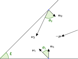
Figure 2: The wedge with the reflection parameters and the drift.

To apply Theorem 1 of Dieker and Moriarty [8], first we transform (41) and (42) into $\overline{R}_{1}(\cdot)=R_{1}(\cdot)/\rho$, $\overline{R}_{2}(\cdot)=R_{2}(\cdot)/\sigma$. The resulting process $(\overline{R}_{1}(\cdot),\overline{R}_{2}(\cdot))$ takes values in

$$\bigl{\{}{(x,y)\in\mathbb{R}^{2}\colon\ 0\leq y\leq\tan(\bolds{\xi})x}\bigr{\}},$$

where we use the notation $\cos(\bolds{\xi})=\sigma$ from (102). The data of the reflection problem become

$$\bolds{\mu} = (h/\rho,-g/\sigma)^{\prime},\qquad\mathbf{n}_{1}=\bolds{\nu}_{1}=(0,1)^{\prime},\qquad\mathbf{n}_{2}=(\rho,-\sigma)^{\prime},\qquad\bolds{\nu}_{2}=(1/\rho,-1/\sigma)^{\prime},$$

$${\bolds{\theta}}_{1} = 0,\qquad{\bolds{\theta}}_{2}=2\bolds{\xi}-\frac{\uppi}{2},\qquad\bolds{\alpha}=\frac{{\bolds{\theta}}_{1}+{\bolds{\theta}}_{2}}{\bolds{\xi}}=2-\frac{\uppi}{2\bolds{\xi}}.$$

The result of Dieker and Moriarty can be applied if $\bm{\alpha}$ is a nonpositive integer $-\ell$, and this amounts to $\bolds{\xi}=\frac{\uppi}{2(\ell+2)}$, that is, $\sigma=\cos(\bolds{\xi})=\cos(\frac{\uppi}{2(\ell+2)})$. In particular,

1. $\bolds{\alpha}=0$, if $\sigma^{2}=1/2$;

2. $\bolds{\alpha}=-1$, if $\sigma^{2}=3/4$; … and

3. $\bolds{\xi}\downarrow 0$, $\bolds{\theta}_{2}\downarrow-\uppi/2$, $\bolds{\alpha}\downarrow-\infty$, as $\sigma^{2}\uparrow 1$ in the limit.

Note that the way of measuring the reflection angles in their paper is to add $\uppi/2$ to the angles $(\bolds{\theta}_{1},\bolds{\theta}_{2})$ of Varadhan and Williams [33] but the parameter $\bolds{\alpha}$ is the same in both papers. Harrison [15], Foschini [14] and Dai and Harrison [7] also studied the stationary distribution of the semimartingale reflected Brownian motion.

$\bullet$ In the case $h>g>0$, $\sigma^{2}=\rho^{2}=1/2$ with $\bolds{\alpha}=0=\ell$, $\bolds{\theta}_{1}=0=\bolds{\theta}_{2}$, we may compute the invariant distribution of the ranks explicitly. From (141), the stationary density function $\mathfrak{p}(\xi_{1},\xi_{2})$ of $(R_{1}(\cdot),R_{2}(\cdot))$ is given by

$$\mathfrak{p}(\xi_{1},\xi_{2})=16h(h-g)\exp\bigl{(}-4(h\xi_{1}-g\xi_{2})\bigr{)},\qquad 0<\xi_{2}<\xi_{1}<\infty.$$ (142)

In fact, by direct computation the second term of (141) is zero. The first term of (141) is proportional to the exponential form $\exp(-2\langle\bolds{\mu},\mathbf{x}\rangle)$. We obtain (142) by observing that $\mathbf{x}=\sqrt{2}(\xi_{1},\xi_{2})^{\prime}$ and $\bm{\mu}=\sqrt{2}(h,-g)^{\prime}$. The value of the normalizing constant comes from the fact that the invariant density of $(R_{1}(\cdot)-R_{2}(\cdot),R_{2}(\cdot))$ is the product of exponentials with parameters $(4h,4(h-g))$.

Remark 9.0.

The skew-symmetry condition of Harrison and Williams [18] holds for the process $(\sqrt{2}R_{1}(\cdot),\sqrt{2}R_{2}(\cdot))$ in the case of equal variances. Under this skew-symmetry condition, the invariant density has the form of a product of exponentials.

These parameters may be derived from the following heuristics. By (3.1) and (41) and the strong law of large numbers for Brownian motion, the local time grows linearly with

$$\lim_{t\to\infty}\bigl{(}L^{R_{2}}(t)/t\bigr{)} = \lim_{t\to\infty}\bigl{(}R_{1}(t)+R_{2}(t)-\xi-\nu t-V(t)\bigr{)}/t=h-g,$$

$$\lim_{t\to\infty}\bigl{(}L^{Y}(t)/t\bigr{)} = h,\qquad\mbox{a.s.}$$

Thus, with these growth rates of the local times, the effective drift rate of $R_{1}(\cdot)-R_{2}(\cdot)$ in (3.1) is heuristically $-\lambda t-\Lambda^{R_{2}}(t)\approx-(g+h)t-(h-g)t=-2ht$ for the large $t>0$. Similarly, from (41) the effective drift rate for $R_{2}(\cdot)$ is $(g-h)/(1/2)=-2(h-g)$, where we divide $(g-h)$ by $1/2$ because the quadratic variation of $\sigma V_{2}(\cdot)$ is a half of that of the standard Brownian motion. Since the invariant density of Brownian motion in $\mathbb{R}_{+}$ with drift rate $-\lambda<0$ reflected at the origin is known to be exponential $(2\lambda)$, we derive the parameters $(4h,4(h-g))$ for $(R_{1}(\cdot)-R_{2}(\cdot),R_{2}(\cdot))$; this is consistent with the consequence of (142) mentioned in the first paragraph of this Remark.

$\bullet$ Similarly, in each case of $\bolds{\alpha}=-\ell$, $\ell\in\mathbb{N}$ we may compute the invariant density of $(R_{1}(\cdot),R_{2}(\cdot))$ from (141). For example, in the case $h>g>0$, $\rho^{2}=1/4$, $\sigma^{2}=3/4$ with

$$\bolds{\alpha}=-1=-\ell,\qquad\bolds{\theta}_{1}=0,\qquad\bolds{\theta}_{2}=-\uppi/6,\qquad\bolds{\xi}=\uppi/6,$$

substituting $\mathbf{x}^{\prime}=(x_{1},x_{2})=(2\xi_{1},2\xi_{2}/\sqrt{3})$ and $\bolds{\mu}^{\prime}=(2h,-2g/\sqrt{3})$ into (141), we obtain for $0<\xi_{2}<\xi_{1}<\infty$ the invariant density $\mathfrak{p}(\xi_{1},\xi_{2})$ of $(R_{1}(\cdot),R_{2}(\cdot))$ as a linear combination of

$$\pi_{0}(\mathbf{x}) \propto \exp\bigl{\{}{-8[{h\xi_{1}-g\xi_{2}/3}]}\bigr{\}},$$

$$\exp\biggl{\{}{-\bolds{\mu}^{\prime}\pmatrix{\frac{3}{2}&-\frac{\sqrt{3}}{2}\cr\frac{\sqrt{3}}{2}&\frac{3}{2}}\mathbf{x}}\biggr{\}} = \exp\bigl{\{}{-\bigl{[}{(6h-2g)\xi_{1}-2(g+h)\xi_{2}}\bigr{]}}\bigr{\}}\quad\mbox{and }$$

$$\exp\biggl{\{}{-\bolds{\mu}^{\prime}\pmatrix{\frac{3}{2}&\frac{\sqrt{3}}{2}\cr\frac{\sqrt{3}}{2}&\frac{1}{2}}\mathbf{x}}\biggr{\}} = \exp\bigl{\{}{-\bigl{[}{(6h-2g)\xi_{1}+(2h-2g/3)\xi_{2}}\bigr{]}}\bigr{\}}.$$

Since $\lim_{\sigma\uparrow 1}\bolds{\alpha}=-\infty$, the invariant distribution of $(R_{1}(\cdot),R_{2}(\cdot))$ in (46), (47) with $\sigma=1$ is conjectured to be proportional to the infinite sum of exponentials as the limit of (141). It is an interesting open problem to determine the invariant distribution for the degenerate case $\sigma^{2}=1$, as well as for general values of $\sigma^{2}$ that correspond to noninteger scalars $\bolds{\alpha}=(\bolds{\theta}_{1}+\bolds{\theta}_{2})/\bolds{\xi}=-\ell$.

Appendix: The other degenerate case, $\sigma=0$

We have assumed throughout this work that the variance of the laggard is positive. In this Appendix, we shall discuss briefly what happens when the laggard undergoes a “ballistic motion” with positive drift $g>0$, and the leader has unit variance, that is $\rho=1$ and $\sigma=0$.

Let us assume then that we have, on some filtered probability space $(\Omega,\mathfrak{F},\mathbb{P}),\mathbf{F}=\{\mathfrak{F}(t)\}_{0\leq t<\infty}$, two continuous, nonnegative and adapted processes $X_{1}(\cdot)$, $X_{2}(\cdot)$ that satisfy

$$\mathrm{d}X_{1}(t) = (g\mathbf{1}_{\{X_{1}(t)\leq X_{2}(t)\}}-h\mathbf{1}_{\{X_{1}(t)>X_{2}(t)\}})\,\mathrm{d}t+\mathbf{1}_{\{X_{1}(t)>X_{2}(t)\}}\,\mathrm{d}V(t),$$ (A.1)

$$\mathrm{d}X_{2}(t) = (g\mathbf{1}_{\{X_{1}(t)>X_{2}(t)\}}-h\mathbf{1}_{\{X_{1}(t)\leq X_{2}(t)\}})\,\mathrm{d}t+\mathbf{1}_{\{X_{1}(t)\leq X_{2}(t)\}}\,\mathrm{d}V(t)+\mathrm{d}\Lambda(t)$$ (A.2)

for $0\leq t<\infty$; here $V(\cdot)$ is standard Brownian motion, and $\Lambda(\cdot)$ is a continuous, adapted and nondecreasing process with $\Lambda(0)=0$ and

$$\int_{0}^{\infty}\mathbf{1}_{\{X_{2}(t)>0\}}\,\mathrm{d}\Lambda(t)=0,\qquad\mbox{a.e.}$$ (A.3)

The system of (A.1), (A.2) corresponds formally to that of (8), (8), in light of the notation (32). No increasing component (such as $\Lambda(\cdot)$ of (A.2)) is needed in (A.1) because, when the process $X_{1}(\cdot)$ finds itself at the origin, the positivity of its drift $g>0$ and the fact that its motion is purely ballistic at that point are sufficient to ensure that $X_{1}(\cdot)$ stays nonnegative.

With the notation of (1), (26) it is fairly clear that the difference $Y(\cdot)=X_{1}(\cdot)-X_{2}(\cdot)$ satisfies the equation

$$\mathrm{d}Y(t)=\operatorname{sgn}\bigl{(}Y(t)\bigr{)}\bigl{(}-\lambda\,\mathrm{d}t+\mathrm{d}V(t)\bigr{)}-\mathrm{d}\Lambda(t);$$ (A.4)

we recall also the Tanaka formulae $\mathrm{d}Y^{+}(t)=\mathbf{1}_{\{Y(t)>0\}}\,\mathrm{d}Y(t)+\mathrm{d}L^{Y}(t)$ and (16), the latter written now in the form

$$\mathrm{d}\big{|}Y(t)\big{|}=-\lambda\,\mathrm{d}t+\mathrm{d}V(t)-\operatorname{sgn}\bigl{(}Y(t)\bigr{)}\,\mathrm{d}\Lambda(t)+2\,\mathrm{d}L^{Y}(t).$$ (A.5)

With their help, we express the rankings of (39) as

$$R_{1}(t) = X_{2}(t)+Y^{+}(t)=r_{1}-ht+V(t)+\int_{0}^{t}\mathbf{1}_{\{X_{1}(s)\leq X_{2}(s)\}}\,\mathrm{d}\Lambda(s)+L^{Y}(t),$$ (A.6)

$$R_{2}(t) = X_{1}(t)-Y^{+}(t)=r_{2}+gt+\int_{0}^{t}\mathbf{1}_{\{X_{1}(s)>X_{2}(s)\}}\,\mathrm{d}\Lambda(s)-L^{Y}(t).$$ (A.7)

We claim that we have the $\mathbb{P}$-a.e. identities

$$\int_{0}^{\infty}\mathbf{1}_{\{X_{1}(t)=X_{2}(t)\}}\,\mathrm{d}t=0,\qquad\int_{0}^{\infty}\mathbf{1}_{\{X_{1}(t)\neq X_{2}(t)\}}\,\mathrm{d}\Lambda(t)=0.$$ (A.8)

Indeed, the first identity is a direct consequence of (2) and (A.5). As for the second, we observe that for any point $t$ at which $\mathbf{1}_{\{X_{1}(\cdot)>X_{2}(\cdot)\}}\,\mathrm{d}\Lambda(\cdot)$ increases, we have $X_{2}(t)=0$, thus $R_{2}(t)=0$; but since $g>0$, we see from (A.7) that $t$ must then be also a point of increase for $L^{Y}(\cdot)$, therefore $X_{1}(t)-X_{2}(t)=Y(t)=0$. We conclude $\int_{0}^{\infty}\mathbf{1}_{\{X_{1}(t)>X_{2}(t)\}}\,\mathrm{d}\Lambda(t)\equiv 0$, thus

$$\Lambda(\cdot)=\int_{0}^{\cdot}\mathbf{1}_{\{X_{1}(t)\leq X_{2}(t)=0\}}\,\mathrm{d}\Lambda(t)=\int_{0}^{\cdot}\mathbf{1}_{\{R_{1}(t)=0\}}\,\mathrm{d}\Lambda(t)$$

in conjunction with (A.3), and so

$$\mathrm{d}(R_{1}-R_{2})(t)=-\lambda\,\mathrm{d}t+\mathrm{d}V(t)-\mathbf{1}_{\{R_{1}(t)=0\}}\,\mathrm{d}\Lambda(t)+2\,\mathrm{d}L^{Y}(t);$$

a comparison with (A.5) gives now the second identity of (A.8). In particular, we have shown that the process $\Lambda(\cdot)$ is supported on the set of visits by the process $(X_{1}(\cdot),X_{2}(\cdot))$ to the corner of the quadrant:

$$\operatorname{supp}\bigl{(}\Lambda(\cdot)\bigr{)}\subseteq\bigl{\{}t\geq 0\colon\ R_{1}(t)=0\bigr{\}}\subseteq\bigl{\{}t\geq 0\colon\ R_{2}(t)=0\bigr{\}}.$$ (A.9)

After all this, the equations of (A.6), (A.7) take the particularly simple form

$$R_{1}(t)=r_{1}-ht+V(t)+\Lambda(t)+L^{Y}(t),\qquad R_{2}(t)=r_{2}+gt-L^{Y}(t),$$ (A.10)

and give

$$X_{1}(t)+X_{2}(t) = R_{1}(t)+R_{2}(t)=\xi+\nu t+V(t)+\Lambda(t),$$ (A.11)

$$R_{1}(t)-R_{2}(t) = |y|-\lambda t+V(t)+\Lambda(t)+2L^{Y}(t).$$ (A.12)

$\bullet$ We observe from (A.9), (2) that $\operatorname{supp}(\Lambda(\cdot)+2L^{Y}(\cdot))\subseteq\{t\geq 0\colon\ R_{1}(t)-R_{2}(t)=0\}$, so it follows from (A.12) that the process $R_{1}(\cdot)-R_{2}(\cdot)\geq 0$ is the Skorokhod reflection at the origin of the Brownian motion with negative drift

$$Z(t)=|y|-\lambda t+V(t),\qquad 0\leq t<\infty,$$ (A.13)

namely

$$\Lambda(t)+2L^{Y}(t)=\max_{0\leq s\leq t}\bigl{(}-Z(s)\bigr{)}^{+}=\max_{0\leq s\leq t}\bigl{(}-|y|+\lambda s-V(s)\bigr{)}^{+},\qquad 0\leq t<\infty.$$ (A.14)

$\bullet$ On the other hand, we observe from (A.10) that

$$0\leq 2R_{2}(t)=2r_{2}+2gt-\bigl{(}\Lambda(t)+2L^{Y}(t)\bigr{)}+\Lambda(t),\qquad 0\leq t<\infty,$$

so in light of (A.9) and the theory of the Skorokhod reflection problem once again, we obtain

$$\Lambda(t)=\max_{0\leq s\leq t}\bigl{(}-2r_{2}-2gs+\Lambda(s)+2L^{Y}(s)\bigr{)}^{+},\qquad 0\leq t<\infty.$$ (A.15)

Remark A.0.

Likewise, from (A.9) the support of $\Lambda(\cdot)$ is included in the zero-set of the process $R_{1}(\cdot)+R_{2}(\cdot)\geq 0$; then (A.11) and the theory of the Skorokhod reflection problem give

$$\Lambda(t)=\max_{0\leq s\leq t}\bigl{(}-\xi-\nu s-V(s)\bigr{)}^{+},\qquad 0\leq t<\infty.$$ (A.16)

In other words, the sum $X_{1}(\cdot)+X_{2}(\cdot)=R_{1}(\cdot)+R_{2}(\cdot)$ is Brownian motion with drift $\nu=g-h$ and reflection at the origin; we are indebted to Dr. Phillip Whitman for this observation.

Consequently, if $h\geq g$, the process $(X_{1}(\cdot),X_{2}(\cdot))$ visits the corner of the nonnegative quadrant with probability one; whereas, if $h<g$, we have

$$\mathbb{P}\bigl{(}X_{1}(t)=X_{2}(t)=0,\mbox{for some }t\geq 0\bigr{)}=\mathrm{e}^{-2(g-h)\xi}.$$

Remark A.0.

Applying the Tanaka formula (16) to the continuous, nonnegative semimartingales $X_{1}(\cdot)+X_{2}(\cdot)$ in (A.11) and $R_{1}(\cdot)-R_{2}(\cdot)$ in (A.12), we obtain the identifications

$$\Lambda(\cdot)=L^{X_{1}+X_{2}}(\cdot),\qquad\Lambda(\cdot)+2L^{Y}(\cdot)=L^{R_{1}-R_{2}}(\cdot),$$ (A.17)

thus also

$$L^{|X_{1}-X_{2}|}(\cdot)-2L^{X_{1}-X_{2}}(\cdot)=L^{X_{1}+X_{2}}(\cdot).$$

On the other hand, we have the $\mathbb{P}$-a.e. properties $\int_{0}^{\infty}\mathbf{1}_{\{R_{1}(t)=0\}}\,\mathrm{d}t=0$, $\int_{0}^{\infty}\mathbf{1}_{\{R_{1}(t)=R_{2}(t)\}}\,\mathrm{d}t=0$ from (A.10), (A.12) and (2). In conjunction with (12) and (10) – in particular, the fact that $L^{X}(\cdot)\equiv 0$ holds for a continuous semimartingale $X(\cdot)$ of finite variation – we obtain from these equations and (A.9) the identifications

$$L^{R_{1}}(\cdot) = \int_{0}^{\cdot}\mathbf{1}_{\{R_{1}(t)=0\}}\,\mathrm{d}R_{1}(t)=\Lambda(\cdot)+\int_{0}^{\cdot}\mathbf{1}_{\{R_{1}(t)=0\}}\,\mathrm{d}L^{Y}(t),$$

$$0=L^{R_{2}}(\cdot) = \int_{0}^{\cdot}\mathbf{1}_{\{R_{2}(t)=0\}}\,\mathrm{d}R_{2}(t)=g\int_{0}^{\cdot}\mathbf{1}_{\{R_{2}(t)=0\}}\,\mathrm{d}t-\int_{0}^{\cdot}\mathbf{1}_{\{R_{2}(t)=0\}}\,\mathrm{d}L^{Y}(t),$$

thus also

$$\int_{0}^{\cdot}\mathbf{1}_{\{R_{1}(t)=0\}}\,\mathrm{d}L^{Y}(t)=g\int_{0}^{\cdot}\mathbf{1}_{\{R_{1}(t)=0\}}\,\mathrm{d}t=0,\qquad\Lambda(\cdot)=L^{X_{1}\vee X_{2}}(\cdot).$$ (A.18)

It is rather interesting that the same process $\Lambda(\cdot)$ should do “triple duty”, as the local time of both the sum $X_{1}(\cdot)+X_{2}(\cdot)$ and the maximum $X_{1}(\cdot)\vee X_{2}(\cdot)$, and as the increasing process in the Skorokhod reflection for the minimum $X_{1}(\cdot)\wedge X_{2}(\cdot)$.

Synthesis: Now we can reverse the above steps. Starting with a standard Brownian motion $V(\cdot)$, we define $Z(\cdot)$, $\Lambda(\cdot)$ and $L^{Y}(\cdot)$ via (A.13)–(A.15); then $R_{1}(\cdot)$, $R_{2}(\cdot)$ via (A.10), and

$$G(\cdot):=R_{1}(\cdot)-R_{2}(\cdot)=Z(\cdot)+\Lambda(\cdot)+2L^{Y}(\cdot)$$ (A.19)

as in (A.12). It is clear from (A.14) that this process $G(\cdot)$ is the Skorokhod reflection at the origin of the Brownian motion with negative drift $Z(\cdot)$ in (A.15), thus nonnegative. It is also clear that the process $\Lambda(\cdot)$ satisfies (A.9), as well as (A.16)–(A.18).

On a suitable extension of the probability space we need to find now a continuous semimartingale $Y(\cdot)$ of the form (A.4), with the help of which we can “unfold” the process $G(\cdot)$ of (A.19) in the form $G(\cdot)=|Y(\cdot)|$. Once this has been done we can define

$$X_{1}(\cdot):=R_{2}(\cdot)+Y^{+}(\cdot),\qquad X_{2}(\cdot):=R_{1}(\cdot)-Y^{+}(\cdot)$$

and verify the equations (A.1), (A.2) in a straightforward manner. In order to carry out this unfolding, the method outlined in Section 4.2 is inadequate; it has to be modified as follows.

We enumerate the excursions of $G(\cdot)$ away from the origin, just as before, but now distinguish between those that originate at the corner of the quadrant ($R_{1}=0$), and the rest ($R_{1}>0$). Excursions of the first type are always marked $\Phi=-1$; while excursions of the second type are assigned marks $\Phi=\pm 1$ independently of each other, and with equal probabilities ($1/2$), just as in Section 4.2. The resulting process $Y(\cdot)=\Phi(\cdot)G(\cdot)$ satisfies $G(\cdot)=|Y(\cdot)|$ and

$$\mathrm{d}Y(t) = \overline{\operatorname{sgn}}\bigl{(}Y(t)\bigr{)}\mathbf{1}_{\{R_{1}(t)>0\}}\,\mathrm{d}G(t)-\mathbf{1}_{\{R_{1}(t)=0\}}\,\mathrm{d}G(t)$$

$$= \overline{\operatorname{sgn}}\bigl{(}Y(t)\bigr{)}\mathbf{1}_{\{R_{1}(t)>0\}}\cdot\mathbf{1}_{\{G(t)>0\}}\,\mathrm{d}G(t)-\mathbf{1}_{\{R_{1}(t)=0\}}\cdot\mathbf{1}_{\{R_{1}(t)=R_{2}(t)\}}\,\mathrm{d}(R_{1}-R_{2})(t)$$

$$= \overline{\operatorname{sgn}}\bigl{(}Y(t)\bigr{)}\mathbf{1}_{\{R_{1}(t)>0\}}\cdot\mathbf{1}_{\{G(t)>0\}}\,\mathrm{d}Z(t)-\mathbf{1}_{\{R_{1}(t)=0\}}\,\mathrm{d}L^{R_{1}-R_{2}}(t)$$

$$= \overline{\operatorname{sgn}}\bigl{(}Y(t)\bigr{)}\mathbf{1}_{\{G(t)>0\}}\,\mathrm{d}Z(t)-\mathbf{1}_{\{R_{1}(t)=0\}}\,\mathrm{d}L^{R_{1}-R_{2}}(t)$$

$$= \overline{\operatorname{sgn}}\bigl{(}Y(t)\bigr{)}\bigl{(}-\lambda\,\mathrm{d}t+\mathrm{d}V(t)\bigr{)}-\mathbf{1}_{\{R_{1}(t)=0\}}\bigl{(}\mathrm{d}\Lambda(t)+2\,\mathrm{d}L^{Y}(t)\bigr{)}$$

$$= \operatorname{sgn}\bigl{(}Y(t)\bigr{)}\bigl{(}-\lambda\,\mathrm{d}t+\mathrm{d}V(t)\bigr{)}-\mathrm{d}\Lambda(t),$$

that is, the equation of (A.4), as promised. We have used (12), (A.9), (A.17), (A.18) as well as the $\mathbb{P}$-a.e. properties $\int_{0}^{\infty}\mathbf{1}_{\{G(t)=0\}}\,\mathrm{d}t=0$, $\int_{0}^{\infty}\mathbf{1}_{\{G(t)>0\}}\,\mathrm{d}(G-Z)(t)=0$; the first of these is a consequence of (2), and the second of Skorokhod reflection.

References

- [1] {barticle}[mr] \bauthor\bsnmBanner, \bfnmAdrian D.\binitsA.D., \bauthor\bsnmFernholz, \bfnmRobert\binitsR. &\bauthor\bsnmKaratzas, \bfnmIoannis\binitsI. (\byear2005). \btitleAtlas models of equity markets. \bjournalAnn. Appl. Probab. \bvolume15 \bpages2296–2330. \biddoi=10.1214/105051605000000449, issn=1050-5164, mr=2187296 \bptokimsref \endbibitem
- [2] {barticle}[mr] \bauthor\bsnmBass, \bfnmR. F.\binitsR.F. &\bauthor\bsnmPardoux, \bfnmÉ.\binitsÉ. (\byear1987). \btitleUniqueness for diffusions with piecewise constant coefficients. \bjournalProbab. Theory Related Fields \bvolume76 \bpages557–572. \biddoi=10.1007/BF00960074, issn=0178-8051, mr=0917679 \bptokimsref \endbibitem
- [3] {barticle}[mr] \bauthor\bsnmBhardwaj, \bfnmS.\binitsS. &\bauthor\bsnmWilliams, \bfnmR. J.\binitsR.J. (\byear2009). \btitleDiffusion approximation for a heavily loaded multi-user wireless communication system with cooperation. \bjournalQueueing Syst. \bvolume62 \bpages345–382. \biddoi=10.1007/s11134-009-9119-8, issn=0257-0130, mr=2546421 \bptokimsref \endbibitem
- [4] {bincollection}[mr] \bauthor\bsnmBurdzy, \bfnmKrzysztof\binitsK. &\bauthor\bsnmMarshall, \bfnmDonald\binitsD. (\byear1992). \btitleHitting a boundary point with reflected Brownian motion. In \bbooktitleSéminaire de Probabilités, XXVI. \bseriesLecture Notes in Math. \bvolume1526 \bpages81–94. \baddressBerlin: \bpublisherSpringer. \biddoi=10.1007/BFb0084312, mr=1231985 \bptokimsref \endbibitem
- [5] {barticle}[mr] \bauthor\bsnmBurdzy, \bfnmKrzysztof\binitsK. &\bauthor\bsnmMarshall, \bfnmDonald E.\binitsD.E. (\byear1993). \btitleNonpolar points for reflected Brownian motion. \bjournalAnn. Inst. Henri Poincaré Probab. Stat. \bvolume29 \bpages199–228. \bidissn=0246-0203, mr=1227417 \bptokimsref \endbibitem
- [6] {barticle}[mr] \bauthor\bsnmChen, \bfnmHong\binitsH. (\byear1996). \btitleA sufficient condition for the positive recurrence of a semimartingale reflecting Brownian motion in an orthant. \bjournalAnn. Appl. Probab. \bvolume6 \bpages758–765. \biddoi=10.1214/aoap/1034968226, issn=1050-5164, mr=1410114 \bptokimsref \endbibitem
- [7] {barticle}[mr] \bauthor\bsnmDai, \bfnmJ. G.\binitsJ.G. &\bauthor\bsnmHarrison, \bfnmJ. M.\binitsJ.M. (\byear1992). \btitleReflected Brownian motion in an orthant: Numerical methods for steady-state analysis. \bjournalAnn. Appl. Probab. \bvolume2 \bpages65–86. \bidissn=1050-5164, mr=1143393 \bptokimsref \endbibitem
- [8] {barticle}[mr] \bauthor\bsnmDieker, \bfnmA. B.\binitsA.B. &\bauthor\bsnmMoriarty, \bfnmJ.\binitsJ. (\byear2009). \btitleReflected Brownian motion in a wedge: Sum-of-exponential stationary densities. \bjournalElectron. Commun. Probab. \bvolume14 \bpages1–16. \biddoi=10.1214/ECP.v14-1437, issn=1083-589X, mr=2472171 \bptokimsref \endbibitem
- [9] {barticle}[mr] \bauthor\bsnmDupuis, \bfnmPaul\binitsP. &\bauthor\bsnmWilliams, \bfnmRuth J.\binitsR.J. (\byear1994). \btitleLyapunov functions for semimartingale reflecting Brownian motions. \bjournalAnn. Probab. \bvolume22 \bpages680–702. \bidissn=0091-1798, mr=1288127 \bptokimsref \endbibitem
- [10] {bbook}[mr] \bauthor\bsnmFernholz, \bfnmE. Robert\binitsE.R. (\byear2002). \btitleStochastic Portfolio Theory: Stochastic Modelling and Applied Probability. \bseriesApplications of Mathematics (New York) \bvolume48. \baddressNew York: \bpublisherSpringer. \bidmr=1894767 \bptokimsref \endbibitem
- [11] {btechreport}[author] \bauthor\bsnmFernholz, \bfnmE. R.\binitsE.R. (\byear2011). \btitleTime reversal in an intermediate model. \btypeTechnical report, \binstitutionINTECH Investment Management LLC, Princeton, NJ. \bptokimsref \endbibitem
- [12] {barticle}[author] \bauthor\bsnmFernholz, \bfnmRobert\binitsR., \bauthor\bsnmIchiba, \bfnmTomoyuki\binitsT. &\bauthor\bsnmKaratzas, \bfnmIoannis\binitsI. (\byear2013). \btitleA second-order stock market model. \bjournalAnnals of Finance \bvolume9 \bpages439–454. \biddoi=10.1007/s10436-012-0193-2 \bptokimsref \endbibitem
- [13] {barticle}[author] \bauthor\bsnmFernholz, \bfnmE. R.\binitsE.R., \bauthor\bsnmIchiba, \bfnmT.\binitsT., \bauthor\bsnmKaratzas, \bfnmI.\binitsI. &\bauthor\bsnmProkaj, \bfnmV.\binitsV. (\byear2013). \btitlePlanar diffusions with rank-based characteristics and perturbed Tanaka equations. \bjournalProbab. Theory Related Fields \bvolume156 \bpages343–374. \bidmr=3055262 \bptokimsref \endbibitem
- [14] {barticle}[mr] \bauthor\bsnmFoschini, \bfnmGerard J.\binitsG.J. (\byear1982). \btitleEquilibria for diffusion models of pairs of communicating computers—symmetric case. \bjournalIEEE Trans. Inform. Theory \bvolume28 \bpages273–284. \biddoi=10.1109/TIT.1982.1056473, issn=0018-9448, mr=0651627 \bptokimsref \endbibitem
- [15] {barticle}[mr] \bauthor\bsnmHarrison, \bfnmJ. Michael\binitsJ.M. (\byear1978). \btitleThe diffusion approximation for tandem queues in heavy traffic. \bjournalAdv. in Appl. Probab. \bvolume10 \bpages886–905. \biddoi=10.2307/1426665, issn=0001-8678, mr=0509222 \bptokimsref \endbibitem
- [16] {barticle}[mr] \bauthor\bsnmHarrison, \bfnmJ. Michael\binitsJ.M. &\bauthor\bsnmReiman, \bfnmMartin I.\binitsM.I. (\byear1981). \btitleReflected Brownian motion on an orthant. \bjournalAnn. Probab. \bvolume9 \bpages302–308. \bidissn=0091-1798, mr=0606992 \bptokimsref \endbibitem
- [17] {barticle}[mr] \bauthor\bsnmHarrison, \bfnmJ. M.\binitsJ.M. &\bauthor\bsnmWilliams, \bfnmR. J.\binitsR.J. (\byear1987). \btitleBrownian models of open queueing networks with homogeneous customer populations. \bjournalStochastics \bvolume22 \bpages77–115. \biddoi=10.1080/17442508708833469, issn=0090-9491, mr=0912049 \bptokimsref \endbibitem
- [18] {barticle}[mr] \bauthor\bsnmHarrison, \bfnmJ. M.\binitsJ.M. &\bauthor\bsnmWilliams, \bfnmR. J.\binitsR.J. (\byear1987). \btitleMultidimensional reflected Brownian motions having exponential stationary distributions. \bjournalAnn. Probab. \bvolume15 \bpages115–137. \bidissn=0091-1798, mr=0877593 \bptokimsref \endbibitem
- [19] {barticle}[mr] \bauthor\bsnmHobson, \bfnmD. G.\binitsD.G. &\bauthor\bsnmRogers, \bfnmL. C. G.\binitsL.C.G. (\byear1993). \btitleRecurrence and transience of reflecting Brownian motion in the quadrant. \bjournalMath. Proc. Cambridge Philos. Soc. \bvolume113 \bpages387–399. \biddoi=10.1017/S0305004100076040, issn=0305-0041, mr=1198420 \bptokimsref \endbibitem
- [20] {barticle}[mr] \bauthor\bsnmIchiba, \bfnmTomoyuki\binitsT. &\bauthor\bsnmKaratzas, \bfnmIoannis\binitsI. (\byear2010). \btitleOn collisions of Brownian particles. \bjournalAnn. Appl. Probab. \bvolume20 \bpages951–977. \biddoi=10.1214/09-AAP641, issn=1050-5164, mr=2680554 \bptokimsref \endbibitem
- [21] {barticle}[author] \bauthor\bsnmIchiba, \bfnmT.\binitsT., \bauthor\bsnmKaratzas, \bfnmI.\binitsI. &\bauthor\bsnmShkolnikov, \bfnmM.\binitsM. (\byear2011). \btitleStrong solutions of stochastic equations with rank-based coefficients. \bjournalProbab. Theory Related Fields \bvolume156 \bpages229–248. \bidmr=3055258 \bptokimsref \endbibitem
- [22] {barticle}[mr] \bauthor\bsnmIchiba, \bfnmTomoyuki\binitsT., \bauthor\bsnmPapathanakos, \bfnmVassilios\binitsV., \bauthor\bsnmBanner, \bfnmAdrian\binitsA., \bauthor\bsnmKaratzas, \bfnmIoannis\binitsI. &\bauthor\bsnmFernholz, \bfnmRobert\binitsR. (\byear2011). \btitleHybrid atlas models. \bjournalAnn. Appl. Probab. \bvolume21 \bpages609–644. \biddoi=10.1214/10-AAP706, issn=1050-5164, mr=2807968 \bptokimsref \endbibitem
- [23] {bbook}[mr] \bauthor\bsnmKaratzas, \bfnmIoannis\binitsI. &\bauthor\bsnmShreve, \bfnmSteven E.\binitsS.E. (\byear1991). \btitleBrownian Motion and Stochastic Calculus, \bedition2nd ed. \bseriesGraduate Texts in Mathematics \bvolume113. \baddressNew York: \bpublisherSpringer. \biddoi=10.1007/978-1-4612-0949-2, mr=1121940 \bptokimsref \endbibitem
- [24] {barticle}[mr] \bauthor\bsnmKruk, \bfnmLukasz\binitsL., \bauthor\bsnmLehoczky, \bfnmJohn\binitsJ., \bauthor\bsnmRamanan, \bfnmKavita\binitsK. &\bauthor\bsnmShreve, \bfnmSteven\binitsS. (\byear2007). \btitleAn explicit formula for the Skorokhod map on . \bjournalAnn. Probab. \bvolume35 \bpages1740–1768. \biddoi=10.1214/009117906000000890, issn=0091-1798, mr=2349573 \bptokimsref \endbibitem
- [25] {barticle}[mr] \bauthor\bsnmKrylov, \bfnmN. V.\binitsN.V. (\byear2004). \btitleOn weak uniqueness for some diffusions with discontinuous coefficients. \bjournalStochastic Process. Appl. \bvolume113 \bpages37–64. \biddoi=10.1016/j.spa.2004.03.012, issn=0304-4149, mr=2078536 \bptokimsref \endbibitem
- [26] {barticle}[mr] \bauthor\bsnmManabe, \bfnmShojiro\binitsS. &\bauthor\bsnmShiga, \bfnmTokuzo\binitsT. (\byear1973). \btitleOn one-dimensional stochastic differential equations with non-sticky boundary conditions. \bjournalJ. Math. Kyoto Univ. \bvolume13 \bpages595–603. \bidissn=0023-608X, mr=0346907 \bptokimsref \endbibitem
- [27] {bincollection}[mr] \bauthor\bsnmOuknine, \bfnmY.\binitsY. (\byear1990). \btitleTemps local du produit et du sup de deux semimartingales. In \bbooktitleSéminaire de Probabilités, XXIV, 1988/89. \bseriesLecture Notes in Math. \bvolume1426 \bpages477–479. \baddressBerlin: \bpublisherSpringer. \biddoi=10.1007/BFb0083790, mr=1071565 \bptokimsref \endbibitem
- [28] {barticle}[mr] \bauthor\bsnmOuknine, \bfnmYoussef\binitsY. &\bauthor\bsnmRutkowski, \bfnmMarek\binitsM. (\byear1995). \btitleLocal times of functions of continuous semimartingales. \bjournalStochastic Anal. Appl. \bvolume13 \bpages211–231. \biddoi=10.1080/07362999508809392, issn=0736-2994, mr=1324099 \bptokimsref \endbibitem
- [29] {barticle}[mr] \bauthor\bsnmProkaj, \bfnmVilmos\binitsV. (\byear2009). \btitleUnfolding the Skorohod reflection of a semimartingale. \bjournalStatist. Probab. Lett. \bvolume79 \bpages534–536. \biddoi=10.1016/j.spl.2008.09.029, issn=0167-7152, mr=2494646 \bptokimsref \endbibitem
- [30] {barticle}[mr] \bauthor\bsnmReiman, \bfnmMartin I.\binitsM.I. (\byear1984). \btitleOpen queueing networks in heavy traffic. \bjournalMath. Oper. Res. \bvolume9 \bpages441–458. \biddoi=10.1287/moor.9.3.441, issn=0364-765X, mr=0757317 \bptokimsref \endbibitem
- [31] {barticle}[mr] \bauthor\bsnmReiman, \bfnmM. I.\binitsM.I. &\bauthor\bsnmWilliams, \bfnmR. J.\binitsR.J. (\byear1988). \btitleA boundary property of semimartingale reflecting Brownian motions. \bjournalProbab. Theory Related Fields \bvolume77 \bpages87–97. \biddoi=10.1007/BF01848132, issn=0178-8051, mr=0921820 \bptokimsref \endbibitem
- [32] {bbook}[mr] \bauthor\bsnmStroock, \bfnmDaniel W.\binitsD.W. &\bauthor\bsnmVaradhan, \bfnmS. R. Srinivasa\binitsS.R.S. (\byear1979). \btitleMultidimensional Diffusion Processes. \bseriesGrundlehren der Mathematischen Wissenschaften [Fundamental Principles of Mathematical Sciences] \bvolume233. \baddressBerlin: \bpublisherSpringer. \bidmr=0532498 \bptokimsref \endbibitem
- [33] {barticle}[mr] \bauthor\bsnmVaradhan, \bfnmS. R. S.\binitsS.R.S. &\bauthor\bsnmWilliams, \bfnmR. J.\binitsR.J. (\byear1985). \btitleBrownian motion in a wedge with oblique reflection. \bjournalComm. Pure Appl. Math. \bvolume38 \bpages405–443. \biddoi=10.1002/cpa.3160380405, issn=0010-3640, mr=0792398 \bptokimsref \endbibitem
- [34] {barticle}[mr] \bauthor\bsnmWilliams, \bfnmR. J.\binitsR.J. (\byear1987). \btitleReflected Brownian motion with skew symmetric data in a polyhedral domain. \bjournalProbab. Theory Related Fields \bvolume75 \bpages459–485. \biddoi=10.1007/BF00320328, issn=0178-8051, mr=0894900 \bptokimsref \endbibitem
- [35] {barticle}[mr] \bauthor\bsnmYan, \bfnmJia An\binitsJ.A. (\byear1980). \btitleSome formulas for the local time of semimartingales. \bjournalChinese Ann. Math. \bvolume1 \bpages545–551. \bidmr=0619601 \bptokimsref \endbibitem
- [36] {barticle}[mr] \bauthor\bsnmYan, \bfnmJia An\binitsJ.A. (\byear1985). \btitleA formula for local times of semimartingales. \bjournalNortheast. Math. J. \bvolume1 \bpages138–140. \bidissn=1000-1778, mr=0834059 \bptokimsref \endbibitem