Schrödinger equations with indefinite effective mass

Miloslav Znojil

Nuclear Physics Institute of Academy of Sciences of the Czech Republic, 250 68 Řež, Czech Republic,

email: znojil @ ujf.cas.cz

phone: 00420 266173286

and

Géza Lévai

Institute of Nuclear Research of the Hungarian Academy of Sciences (ATOMKI),

PO Box 51, H-4001 Debrecen, Hungary

email: levai @ namafia.atomki.hu

Abstract

The consistency of the concept of quantum (quasi)particles possessing effective mass which is both position- and excitation-dependent is analyzed via simplified models. It is shown that the system may be stable even when the effective mass $m=m(x,E)$ itself acquires negative values in a limited range of coordinates $x$ and energies $E$.

1 Introduction

Non-relativistic quantum dynamics of point particles is most often studied via ordinary differential Schrödinger equation

$$-\frac{\ \hbar^{2}}{2m}\frac{d^{2}}{d{x}^{2}}\,\Psi(x)+V(x)\,\Psi(x)=E\,\Psi(x)\,,\ \ \ \ \ \ \ \Psi(x)\in L^{2}(\mathbb{R})$$ (1)

where the real function $V(x)$ characterizes an external local potential while the particle mass $m>0$ is just a given constant. Various generalized forms of this equation were introduced due to the practical needs of the description of motion of a particle or quasiparticle inside a medium. The medium may make the mass position-dependent [1]. The phenomenological appeal of the spatial variability of the effective mass is accompanied by some additional formal merits of the generalization, say, in the context of supersymmetric quantum mechanics [2].

In the majority of papers which studied the models with $m=m(x)$ the authors assumed that $m(x)>0$ [3]. The more we were surprised when we found [4] that in the so called ${\cal PT}-$symmetric version of the quantum Coulomb problem the stability of the system required an anomalous, asymptotically negative choice of the coordinate-dependent effective mass. This observation re-attracted our attention to quantum models with $m=m(x)$ and, in particular, to their subset in which one encounters the anomalous $m(x)<0$, in some nonempty interval of coordinates at least.

In what follows we intend to describe some results of our analysis. Firstly, in section 2 we introduce an elementary solvable Schrödinger equation with a piecewise constant mass such that $m=m(x)<0$ for $x\in(-1,1)$. We shall demonstrate that the bound-state spectrum of energies of such a model is unbounded from below so that the model cannot be interpreted as realistic due to its immanent instability. This result supports our expectations that for the models with indefinite mass $m(x)$ such an instability will be generic.

One of the possible methods of elimination of similar pathologies is then proposed in section 3. We recall the general Feshbach’s definition of the effective quantities in quantum theory (cf. ref. [5]) and conjecture that the apparent anomalies in the behavior of the benchmark square-well model of section 2 are not realistic. We argue that their emergence should be attributed to our unfounded complete suppression of the necessary variability of the effective mass with the energy. On this basis we propose and describe our first exactly solvable model with $m=m(x,E)$ in section 3 and its alternative version in section 4.

Our main result is that both of these amended benchmark models may remain stable (and, hence, acceptable for phenomenological purposes), provided only that the mass $m(x,E)$ stays merely anomalous (i.e., negative) in a restricted range of its arguments (i.e., in finite intervals of coordinates $x$ and energies $E$).

A few formal aspects and possible consequences of the reinstalled mathematical consistency and acceptability of Schrödinger equations with sign-changing effective masses $m(x,E)$ will be finally mentioned in section 5. We shall re-emphasize there the phenomenological as well as purely theoretical appeal of the use of effective masses $m(x,E)$ which change their sign. Whenever it happens just locally in both $x$ and $E$, one may encounter no contradiction with expectations and/or with the general principles of quantum mechanics.

2 The instability of quantum systems with a locally negative effective mass $m=m(x)$

In the majority of applications one accepts the requirement of the positivity of the mass $m(x)>0$ as natural. In the light of Ref. [4], such a rule might have its exceptions. We should admit that in the latter paper the weird-looking asymptotic negativity of the effective mass can in fact be attributed to our rather technical postulate of the loss of the observability of the coordinate $x$ in the asymptotic region [6]. Vice versa, we believe that the effective mass $m(x)$ should remain asymptotically positive whenever the asymptotic coordinates $x$ remain real. In this context, our present letter may be read as motivated by the question of possible existence of some physically consistent scenarios admitting a negative effective mass $m(x)<0$, say, in some not too large finite interval of coordinate $x\in\mathbb{R}$.

For the sake of definiteness let us simplify the mathematics of such a conceptual problem by considering just the toy model in which the energy spectrum is discrete and in which one works with the deep square-well potential

$$V(x)=\left\{\begin{array}[]{cc}+\infty,&\ \ \ |x|>L>1\,,\\ 0,&\ \ \ |x|<L\,.\end{array}\right.$$ (2)

Moreover, in our models the mass will be piecewise constant, say, as follows,

$$m(x)=\left\{\begin{array}[]{cc}1,&\ \ \ |x|\in(1,L)\,,\\ m_{0},&\ \ \ |x|<1\,.\end{array}\right.$$ (3)

Unfortunately, whenever $m_{0}$ is negative, the spectrum of the bound-state energies of such a model becomes unbounded from below. This makes the whole system unstable with respect to perturbations so that its physical meaning becomes highly questionable. Still, it makes good sense to understand this counterintuitive and apparently discouraging fact in a more quantitative detail.

Let us consider the toy-model Schrödinger equation

$$-\frac{\ \hbar^{2}}{2m(x)}\frac{d^{2}}{d{x}^{2}}\,\Psi(x)+V(x)\,\Psi(x)=E\,\Psi(x)\,$$ (4)

with potential (2) and mass (3) where, say, $m_{0}=-1$. Let us also restrict our attention, for the sake of brevity, to the mere even-parity bound-state solutions $\Psi(x)=\Psi(-x)$ such that $\Psi(-L)=\Psi(L)=0$.

In units $\hbar^{2}/2=1$ and in the first step of analysis we shall assume that $E=k^{2}$ is non-negative. This means that we have to solve two differential equations,

$$\begin{array}[]{cc}-\frac{d^{2}}{d{x}^{2}}\,\Psi(x)=k^{2}\,\Psi(x)&\ \ x\in(-L,-1)\,,\\ -\frac{d^{2}}{d{x}^{2}}\,\Psi(x)=-k^{2}\,\Psi(x)&\ \ x\in(-1,0)\,,\end{array}$$ (5)

with the respective explicit solutions

$$\begin{array}[]{cc}\Psi(x)=\sin k(x+L)&\ \ x\in(-L,-1)\,,\\ \Psi(x)=D\,{\rm cosh}\,kx&\ \ x\in(-1,0)\end{array}$$ (6)

which satisfy the usual physical boundary conditions. In addition, these solutions must also satisfy the usual mathematical matching conditions at $x=-1$,

$$\begin{array}[]{c}D\,{\rm cosh}\,k=\sin k(L-1)\,,\\ -D\,{\rm sinh}\,k=\cos k(L-1)\,.\end{array}$$ (7)

This determines the eigenvalues $E_{n}=k^{2}_{n}$ via an elementary transcendental equation

$${\rm tanh}\,k\times\tan k(L-1)=-1\,$$ (8)

(cf. the two samples of its graphical solution in Fig. 1).

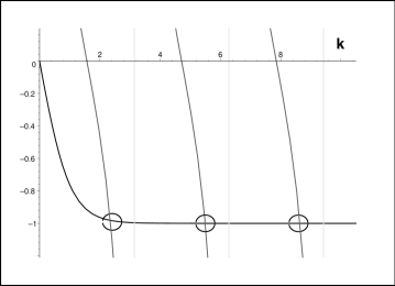
Figure 1: Graphical solution of Eq. (8) at $L=2$ (the small circles mark the intersections of $-{\rm tanh}\,k$ with $\cot k(L-1)$).

In the same units $\hbar^{2}/2=1$ and in the second step let us set $E=-\kappa^{2}$ and write down the two corresponding equations,

$$\begin{array}[]{cc}-\frac{d^{2}}{d{x}^{2}}\,\Psi(x)=-\kappa^{2}\,\Psi(x)&\ \ x\in(-L,-1)\,,\\ -\frac{d^{2}}{d{x}^{2}}\,\Psi(x)=\kappa^{2}\,\Psi(x)&\ \ x\in(-1,0)\,,\end{array}$$ (9)

with the respective explicit solutions

$$\begin{array}[]{cc}\Psi(x)={\rm sinh}\,\kappa(x+L)&\ \ x\in(-L,-1)\,,\\ \Psi(x)=F\,\cos\,\kappa x&\ \ x\in(-1,0)\,.\end{array}$$ (10)

The matching conditions at $x=-1$ yield the two constraints,

$$\begin{array}[]{c}{\rm sinh}\,\kappa(L-1)=F\,\cos\kappa\,,\\ {\rm cosh}\,\kappa(L-1)=F\,\sin\kappa\,.\end{array}$$ (11)

The resulting implicit definition of the negative-energy eigenvalues $E_{n}=-\kappa^{2}_{n}$ is then obtained,

$$\tan\kappa\times{\rm tanh}\,\kappa(L-1)=1\,$$ (12)

and yields infinitely many roots again (cf. their graphical representation in Fig. 2). Hence, the spectrum appears unbounded from below. This forces us to declare the model manifestly unphysical.

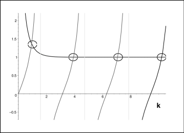
Figure 2: Graphical solution of Eq. (12) at $L=2$ (the small circles mark the intersections of $\tan k$ with $\coth k(L-1)$).

The key role of our particular example (3) possessing the discrete bound-state spectrum which is not bounded below should be seen in its methodical importance. Indeed, although the model is mathematically correct, its stability will be immediately lost under the influence of virtually arbitrary perturbation.

Naturally, such a feature of our toy model is generic. Moreover, its instability under perturbations might have been expected a priori since, after the kinetic energy becomes negative, the perturbed system will certainly have a tendency of plunging, spontaneously, into the lower and lower energy states. The corresponding wave functions will acquire a highly oscillatory form.

Qualitatively, the perturbative instability phenomenon will remain the same for virtually any external potential $V(x)$. The exact solvability of our model gives such a sensitivity to perturbations just a fully explicit form. For our particular constant and energy-independent choice of the parameter $m_{0}<0$ one observes the explicit form of the steady increase of the localization of the unperturbed wave functions inside the non-empty interval of $x$. With the growth of parameter $\kappa$ we merely witness the emergence of an explicit square-well-like part of the bound-state spectrum which is turned upside down.

3 A realistic, energy-dependent model

In the language of physics, the unperturbed versions of our simple-minded $m_{0}<0$ toy model should be re-interpreted as incomplete. Any realistic realization of similar systems (which, in principle, radiate, i.e., act as a source of energy) must necessarily be reconsidered as coupled to an environment. In other words, we must re-classify our physical Hilbert space as a mere subspace ${\cal H}_{P}$ of a larger physical Hilbert space ${\cal H}^{full}$.

The lack of the knowledge of the (usually, prohibitively complicated) full Hamiltonian $H^{full}$ which would characterize the environment (and which would act in the full Hilbert space ${\cal H}^{full}$) leads to the necessity of acceptance of some hypotheses. Fortunately, the use of the formalism of the Feshbach’s projection-operator techniques (cf. [5] for details) appears extremely efficient in this context.

For our present purposes, in particular, is it sufficient to take into account that even if the rigorously known spectrum of our unperturbed, decoupled (or, in the Feshbach’s language, $P-$projected) Hamiltonian of section 2 is not bounded from below, any of its realistic perturbed versions may be given the Feshbach’s semi-explicit form

$$H^{(effective)}=P\,H^{full}\,P+P\,H^{full}\,Q\,\frac{1}{E-Q\,H^{full}\,Q}\,Q\,H^{full}\,P\,$$ (13)

where $Q=I-P$. Such an effective Hamiltonian may certainly represent measurable phenomena but, by assumption, our knowledge of this operator is restricted and incomplete. Its important merit is that it is still defined in the accessible, “small”, $P-$projected Hilbert space ${\cal H}_{P}$. Next, the energy $E$ need not be considered complex in the present setting. The reason is that we may and shall tacitly assume that the whole spectrum of $H^{full}$ remains discrete and that, for the sake of simplicity, the energy $E$ in (13) does not belong to the spectrum of $Q\,H^{full}\,Q$.

The only conclusion which we can make about the difference between the schematic, unperturbed negative-mass Hamiltonian (say, $P\,H^{full}\,P$) and the whole family of its possible realistic effective descendants (13) is that all of the latter operators must be, necessarily, manifestly energy-dependent. This fact may be recalled as giving the reasons why the choice of the effective mass should also be considered energy-dependent in general. Vice versa, once we admit that the mass is energy dependent, $m=m(x,E)$, any restriction of attention just to the positive values of this phenomenological parameter becomes entirely artificial.

Via our previous, energy-independent example we already understand that the emergence of the unlimited decrease of the sequence of the bound-state energy levels should be attributed to the purely mathematical role played by the negative constant $m_{0}<0$ at the large parameters $E=-\kappa^{2}$. On this basis we may most simply stabilize the spectrum by keeping the effective mass positive beyond certain threshold, $m(x,E)>0$ for $E<E_{thr}$.

In parallel, the physical meaning of the threshold energy cut-off may vary with the hypotheses concerning the environment. The choice of its value may be interpreted as a compressed information about the interplay between the complicated coupling operators $P\,H^{full}\,Q$ and the Hamiltonian of the environment $Q\,H^{full}\,Q$. Naturally, even such a weak form of information about the hidden and/or prohibitively complicated dynamical mechanisms may still play the role of a phenomenological source of variability of the effective mass.

Needless to add, the use of the energy-dependent effective operators finds a broad range of applications in various domains of quantum physics [7]. The key feature of their Feshbach’s mathematical origin is that every effective operator (defined in the $P-$projected subspace) varies with the changes of the energy of the $(P+Q)-$projected system. In this sense, the unwanted emergence of mathematical anomalies (like, typically, the unbounded spectrum as mentioned above) may still be eliminated and attributed to an inappropriate treatment of the energy-dependent simulation of the effects of the environment.

For the sake of definiteness of our argument let us now proceed by teaching by example again, replacing the constant parameter $m_{0}$ in Eq. (3) by its suitable energy-dependent generalization. It will be allowed negative at $E>E_{thr}$ for, say, $E_{thr}=0$. For the sake of simplicity, let us also add the convenient assumption that $m_{0}(E)\to 1$ for $E\to-\infty$ and that $m_{0}(E)\to-1$ for $E\to+\infty$.

Under these assumptions, we may select, for illustration purposes, the following, most elementary interpolation ansatz replacing Eq. (3),

$$m(x,E)=\left\{\begin{array}[]{cc}1,&\ \ \ |x|\in(1,L)\,,\\ -{\rm tanh}\,(E),&\ \ \ |x|<1\,.\end{array}\right.$$ (14)

Under this choice the value of the mass parameter just simulates the emergence of an anomaly in the kinetic-energy operator for a restricted range of the energies. As already mentioned, such an effective kinetic-energy operator finds its natural hypothetical origin in the Feshbach’s reduction of a realistic or “complete” (i.e., formally, $(P+Q)-$projected) Hilbert space (including some unspecified and formally eliminated “medium”) to its suitable, explicitly tractable (i.e., $P-$projected alias model-space) subspace.

In the resulting amended version

$$-\frac{1}{m(x,E)}\frac{d^{2}}{d{x}^{2}}\,\Psi(x)=E\,\Psi(x)\,,\ \ \ \ \ \Psi(-L)=\Psi(L)=0$$ (15)

of our toy-model Schrödinger equation the emergence of energy-dependence of the mass certainly does not change the applicability of the matching method of solution. The insertion of the amended effective mass (14) will still enable us to proceed in an almost complete parallel with the preceding section. First of all we shall split our equation in its “outer” and “inner” part,

$$\begin{array}[]{cc}-\frac{d^{2}}{d{x}^{2}}\,\Psi(x)=E\,\Psi(x)&\ \ x\in(-L,-1)\,,\\ -\frac{d^{2}}{d{x}^{2}}\,\Psi(x)=-E\,{\rm tanh}\,(E)\,\Psi(x)&\ \ x\in(-1,0)\end{array}$$ (16)

and restrict our attention, for the sake of brevity, just to the even-party states again. Next we distinguish between the positive and negative sign of $E$. In the former case we set $E=k^{2}$ yielding the ansatz

$$\begin{array}[]{cc}\Psi(x)=\sin k(x+L)\,,&\ \ x\in(-L,-1)\,,\\ \Psi(x)=D\,{\rm cosh}\,\lambda x\,,&\ \ x\in(-1,0)\,,\ \ \ \ \lambda=\lambda(k)=k\,\sqrt{{\rm tanh}\,k^{2}}>0\,,\end{array}$$ (17)

while in the latter case we put $E=-\kappa^{2}$ and get

$$\begin{array}[]{cc}\Psi(x)={\rm sinh}\,\kappa(x+L)\,,&\ \ x\in(-L,-1)\,,\\ \Psi(x)=F\,{\rm cosh}\,\mu x\,,&\ \ x\in(-1,0)\,,\ \ \ \ \mu=\mu(\kappa)=\kappa\,\sqrt{{\rm tanh}\,\kappa^{2}}>0\,.\end{array}$$ (18)

The respective matching conditions read

$$\begin{array}[]{c}D\,{\rm cosh}\,\lambda(k)=\sin k(L-1)\,,\\ -\lambda(k)\,D\,{\rm sinh}\,\lambda(k)=k\,\cos k(L-1)\,,\end{array}$$ (19)

$$\begin{array}[]{c}{\rm sinh}\,\kappa(L-1)=F\,{\rm cosh}\,\mu(\kappa)\,,\\ \kappa\,{\rm cosh}\,\kappa(L-1)=-\mu(\kappa)\,F\,{\rm sinh}\,\mu(\kappa)\,.\end{array}$$ (20)

They imply that the eigenvalues may be obtained from the respective transcendental equations

$$\sqrt{{\rm tanh}\,k^{2}}\ {\rm tanh}\,\lambda(k)\,\tan k(L-1)=-1\,,$$ (21)

$$\sqrt{{\rm tanh}\,\kappa^{2}}\ {\rm tanh}\,\mu(\kappa)\,{\rm tanh}\,\kappa(L-1)=-1\,.$$ (22)

We see that the left-hand side of the latter equation is nonnegative for any real $\kappa$ so that the set of its roots is empty. The bound-state energies themselves are all determined by Eq. (21) (cf. Fig. 3 which may be perceived as just a slightly deformed analogue of Fig. 1).

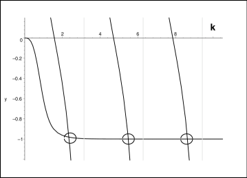
Figure 3: Graphical solution of Eq. (21) at $L=2$.

The even-state part of the spectrum proves bounded from below. This is our main conclusion. Along similar lines, the same conclusion may be obtained for the odd-parity bound states. We may summarize that whenever one wants to work with the quantum systems in which the effective mass can get negative, one is not allowed to neglect the variability of the effective mass with the energy.

4 Another exactly solvable model

The introduction of the energy-dependence in the effective mass has been based on the existence of a hypothetical environment. One would expect, on this basis, that the “realistic” $E-$dependence of $m(x,E)$ would be smooth. In such a case, the study of the related ordinary differential effective Schrödinger equations may proceed in parallel with the $E-$independent cases. A compact review of these parallels may be found in Ref. [8]. It has been emphasized there that the overlaps between the wave functions corresponding to different energies will not vanish in general. In our present particular model the readers might easily check this fact using the available explicit formulae for wave functions.

An exhaustive clarification of this apparent paradox may be found in Ref. [8]. Interested readers find there not only the standard Hilbert-space interpretation of the energy-dependent Hamiltonians (based on the use of suitably adapted ad hoc inner products) but also the explicit realization of the bi-orthogonality and bi-orthonormality relations between eigenstates in similar models. One of the most concise reviews of the extension of this formalism to the case of the general non-Hermitian observables may be also found in Ref. [9].

We saw, via the schematic illustrative example of preceding section, that the bound-state spectrum might be very sensitive to the value of the threshold energy $E_{thr}$. In particular, it may be expected much more sensitive to this value than to the concrete shape of the function $m_{0}(E)$ itself. For this reason, let us now replace the smooth-function ansatz (14) by the simplified but arbitrarily shifted step-function shape

$$m(x,E)=\left\{\begin{array}[]{cc}1,&\ \ \ |x|\in(1,L)\,,\\ \left.\begin{array}[]{cc}-1,&E\geq E_{thr}\\ +1,&E<E_{thr}\end{array}\right\},&\ \ \ |x|<1\end{array}\right.$$ (23)

where the threshold energy is now to be chosen as any finite, real and, for the sake of definiteness, negative variable $E_{thr}=-\beta^{2}$. In this context one must be aware of the fact that for a generic phenomenological potential given in advance, the similar discontinuities and abrupt changes of the mass might give rise to singular contributions to the effective potential. This would deserve a separate analysis. Interested readers are recommended to check the existing literature in this respect [10].

Certainly, there will be no solutions at the energies $E<-\beta^{2}$. For the sake of brevity, we shall again discuss just the even-parity bound states. In this case, the half-infinite interval of the eligible energies should again be split into the high-energy half-line with $E=k^{2}>0$ and the complementary low-energy interval with $E=-\kappa^{2}$ where one must merely admit the limited range of the eligible $\kappa\in(0,\beta)$.

In the former case we may return to Fig. 1, reminding the readers that the high-energy subset of our present, “second-example” eigenvalues $E_{n}=k^{2}_{n}$, $n=1,2,\ldots$ will still be defined as roots of the same, unchanged Eq. (8).

The similar implicit specification of the second, low-energy subset of the remaining eigenvalues $E_{1-n}=\kappa^{2}_{n}$, $n=1,2,\ldots,N$ should again be deduced, mutatis mutandis, from the unmodified secular Eq. (12). The problem is easily resolved since a return to Fig. 2 reveals that we just have to replace the original infinite half-axis of $\kappa$ of section 2 by its finite subinterval of admissible $\kappa\in(0,\beta)$.

We may conclude that the new lowest (i.e., ground-state) energy level will always emerge when there appears a new root of Eq. (12), i.e., the new root $\kappa_{N}=\beta_{critical}$ of equation

$$\tan\beta_{critical}\times{\rm tanh}\,\beta_{critical}(L-1)=1\,.$$ (24)

In other words, with the increase of the real variable $\beta>0$, new and new elements of the sequence of the energies $E_{1-n}=-\kappa_{n}^{2}$ computed in section 2 and sampled in Fig. 2 will be reclassified as the acceptable elements of the spectrum of the present new model.

Special attention must be paid to the limiting case in which $\kappa=\beta_{critical}$. It is necessary to keep in mind that also in such an extreme case the matching condition is satisfied in standard manner so that the related solution has to be accepted as a valid new lowest-lying bound state. Perhaps, it is worth adding that as long as, by our assumption, the effective mass of such a state remains negative in the whole interval of $x\in(-1,1)$, one should not be surprised that such a state is more or less fully localized in this interval. We also see from the explicit formula (10) for wave functions that the number of the nodal zeros of such a wave function, paradoxically, increases with the decrease of $E_{thr}=-\beta_{critical}^{2}$.

5 Discussion

Naturally, our present, methodically motivated restriction of the number of the free parameters to the necessary minimum might be very easily relaxed in any future work. One might point out, for example, that the level-pattern as provided by Fig. 2 is, via secular Eq. (12), closely related to the role and interpretation of the threshold-energy parameter $E_{thr}=-\beta^{2}$ entering our second illustrative example of paragraph 4. This means that the same qualitative picture will be also provided by the trivially rescaled models while the pattern may be changed by an introduction of an additional parameter.

In such a setting it has been extremely interesting for us to notice that the replacement of our one-parametric toy model (2) + (3) by its two-parametric generalization with optional $a>0$ and $b=b(E)>0$ in the effective mass

$$m(x)=\left\{\begin{array}[]{cc}1,&\ \ \ |x|\in(a,L)\,,\\ -1/b^{2},&\ \ \ |x|<a\end{array}\right.$$ (25)

leads to the mere replacement of our previous secular Eq. (12) by the rescaled relation

$$\tan\frac{\kappa a}{b}\times{\rm tanh}\,\kappa(L-a)=b\,.$$ (26)

Naturally, no qualitative changes are encountered for the single rescaling variable $b=a$. Nevertheless, a nontrivial qualitative change of the pattern will emerge in the “deep narrow mass well” regime with small $a$ and $b$ such that also the ratio $a/b:=\nu$ gets small.

In this regime, secular Eq. (26) does not possess any small$-\kappa$ solution so that $\tanh\kappa(L-a)={\cal O}(1)$. One reveals that in the way illustrated by Fig. 2, the sequence of the “larger” roots $\kappa_{2}\approx\pi b/a$, $\kappa_{3}\approx 2\pi b/a$ “disappears” to the right infinity in the limit $\nu=a/b\to 0$. The remaining, single and numerically easily obtainable leftmost root $\kappa_{1}$ will remain finite. Its approximate value will be given by the reduced secular equation

$$\kappa_{1}=\frac{b}{\nu}\,{\rm coth}\,\kappa_{1}L\,.$$ (27)

Obviously, the right-hand-side expression does not change too quickly with $\kappa_{1}$ and it will be, in addition, not too much larger than the ratio $b/\nu$ itself. Thus, typically, for $b/\nu=1$ one obtains, numerically, the approximate value $\kappa_{1}\approx 1.2$ of the root.

One just has to add that in such a special $b=\nu$ limit our mass function (25) with $-1/b^{2}\sim 1/a$ may be interpreted as the Dirac’s delta function so that the survival of just the single bound state in the spectrum might have been, intuitively, expected.

The most important mathematical merit of our present choice of the position-dependent effective masses (which are just piecewise constant functions of $x$) is that the selection of the rigorously defined self-adjoint Hamiltonian is traditional and trivial. In the first two single-parameter toy-models it was provided by the most elementary matching of the logarithmic derivatives of the wave functions. This observation has been complemented by the third example in which we revealed that one could also employ some less trivial matching prescriptions in certain limiting cases.

Still, no use of the full-fledged self-adjoint-extension theory [11] was needed. Due to the piecewise constant nature of our effective masses, we did not even have to consider their usual von Roos’ [12] factorizations $m(x,E)=m_{1}(x,E)\,m_{2}(x,E)\,m_{3}(x,E)$, nor did we have to select an appropriate ordering of the individual mass factors and differential operators $d/dx$ (which, naturally, do not mutually commute in general).

The resulting simplification of the mathematics and of the necessary functional analysis did certainly make the physical interpretation of our models more transparent. This enabled us to emphasize that the Feshbach-method origin of the concept of the effective mass opens several new perspectives in the related phenomenology. In our present letter we managed to demonstrate, first of all, that, and under which conditions, the effective mass $m=m(x,E)$ need not necessarily be required a positive function of $x$ and/or $E$.

We might point out that our present detailed description of a few toy models clarified that there exists an intuitively obvious connection between the violation of the positivity requirement $m(x)>0$ and the breakdown of certain traditional theorems. Let us recall, for example, our observation that in the cases of indefinite $m(x)$, the ground-state wave function is allowed to possess nodal zeros so that the traditional Sturm-Liouville oscillation theorems cease to be valid and must be modified. In parallel, we noticed that in many cases, the anomalous increase of the number of the nodal zeros with the decrease of the bound state energy is accompanied by the perceivable localization of the wave function inside the interval of negativity of $m(x,E)$.

All of these mathematical observations might find their potential future physical applications in all of the phenomenological models where one has to mimic some effects of an (unknown, implicitly described) external medium by means of the use of the (energy-dependent) effective operators. In this context we kept in mind some possible parallels with the relativistic phenomena and with the well known contrast between the behavior of particles and antiparticles. Thus, we concentrated our attention to the toy-model study of the extreme scenario in which the effective kinetic energy reverses its sign.

We may conclude that the oversimplified nature of our illustrative examples served our purposes well. In particular, they helped us to clarify the connection between the decrease of the value of the negativity-threshold energy $E_{thr}$ and the increase of the number of the “anomalous”, localized and quickly-oscillatory low-lying bound states. Via our second example admitting a freely variable $E_{thr}=-\beta^{2}$, this connection has been even quantitatively sampled by the elementary-looking restriction of the pattern given by Fig. 2 to the finite interval of admissible $\kappa\leq\beta$.

References

- [1] G. Bastard, Wave Mechanics Applied to Semiconductor Heterostructure (Les Ulis: Les Editions de Physique, 1988); P. Harrison, Quantum Wells, Wires and Dots, (Wiley, New York, 2000); J-M. Lévy-Leblond, Phys. Rev. A 52 (1995) 1845.
- [2] A. R. Plastino, A. Rigo, M. Casas, F. Garcias and A. Plastino, Phys. Rev. 60 (1999) 4318; B. Bagchi, A. Ganguly and A. Sinha, Phys. Lett. A 374 (2010) 2397.
- [3] G. Lévai and O. Özer, J. Math. Phys. 51 (2010) 092103 and further references contained therein.
- [4] G. Lévai, P. Siegl and M. Znojil, J. Phys. A: Math. Theor. 42 (2009) 295201.
- [5] H. Feshbach, Ann. Phys. (NY) 5 (1958) 357 and 19 (1962) 287.
- [6] M. Znojil, P. Siegl and G. Lévai, Phys. Lett. A 373 (2009) 1921.
- [7] I. Rotter, J. Phys. A: Math. Theor. 42 (2009) 153001.
- [8] M. Znojil, Phys. Lett. A 326 (2004) 70.
- [9] M. Znojil, SIGMA 5 (2009) 001.
- [10] A. Ganguly, M. V. Ioffe and L. M. Nieto, J. Phys. A: Math. Theor. 39 (2006) 14659.
- [11] E. B. Davies, Linear operators and their spectra (Cambridge, Cambridge University Press, 2007).
- [12] O. von Roos, Phys. Rev. B 27 (1983) 7547; B. Bagchi, P. Gorain, C. Quesne and R. Roychoudhury, Mod. Phys. Lett. A 19 (2004) 2765; C. Quesne, Ann. Phys. 321 (2006) 1221.