Fast simulation of truncated Gaussian distributions

Abstract.

We consider the problem of simulating a Gaussian vector $X$, conditional on the fact that each component of $X$ belongs to a finite interval $[a_{i},b_{i}]$, or a semi-finite interval $[a_{i},+\infty)$. In the one-dimensional case, we design a table-based algorithm that is computationally faster than alternative algorithms. In the two-dimensional case, we design an accept-reject algorithm. According to our calculations and our numerical studies, the acceptance rate of this algorithm is bounded from below by $0.5$ for semi-finite truncation intervals, and by $0.47$ for finite intervals. Extension to 3 or more dimensions is discussed.

1. Introduction

Let $X=(X_{1},\ldots,X_{d})$ be a $d-$dimensional Gaussian vector with mean $\mu$ and covariance matrix $\Sigma$, and let $[a_{i},b_{i}]$ be $d$ intervals, where $b_{i}$ may be either a real number or $+\infty$. The distribution of $X$, conditional on the event that $X_{i}\in[a_{i},b_{i}]$, $i=1,\ldots,d$, is usually called a truncated Gaussian distribution (Johnson et al.,, 1994, Chap. 13). Without loss of generality, one may assume that $\mu=0$, and that $\Sigma$ has unit diagonal elements.

Numerous statistical algorithms rely on intensive simulation of truncated Gaussian distributions. In particular, several Bayesian models generate full conditional distributions of this type, either directly or through a data augmentation representation (Tanner and Wong,, 1987). Thus, the corresponding Gibbs samplers (or more generally Markov chain Monte Carlo algorithms) draw repetitively from truncated Gaussian distributions. Examples include linear regression models with ordered parameters (Chen and Deely,, 1996) or applied to truncated data (Gelfand et al.,, 1992), probit models (Albert and Chib,, 1993), multinomial probit models (Albert and Chib,, 1993; McCulloch and Rossi,, 1994; Nobile,, 1998), multivariate probit models (Chib and Greenberg,, 1998), multiranked probit models (Linardakis and Dellaportas,, 2003), tobit models (Chib,, 1992), models used in spectroscopy (Gulam Razul et al.,, 2003), copula regression models (Pitt et al.,, 2006), among others.

To understand how intensive such MCMC algorithms can be, consider the problem of sampling the posterior distribution of a multinomial probit model with $n$ observations and $p$ alternatives. A solution is to perform $T$ iterations of the Gibbs sampler of McCulloch and Rossi, (1994), but this requires the generation of $Tnp$ univariate truncated Gaussian variates, a number that may exceed $10^{12}$ or even $10^{15}$ in difficult scenarios. Hence any improvement with respect to the computational cost of simulating univariate truncated Gaussian distributions may lead to important savings. Another important aspect of such algorithms is that they simulate only one random variable from a given truncated Gaussian distribution, that is, the parameters and the truncation intervals $[a_{i},b_{i}]$ change every time a truncated Gaussian variate is generated. Thus, we are interested in developing specialised algorithms which are guaranteed to generate quickly one random variable from the desired distribution, for all possible inputs (i.e., parameters and truncation intervals). As a corollary, these algorithms cannot afford a long set-up (initialisation) time, where some exploration of the target density is performed in order to improve performance; this type of initialisation is meaningful only when one needs to simulate many variables from one fixed distribution, and is not discussed in this paper. The algorithm we propose does require a table set-up, but which is independent of the input parameters.

The first part of this paper presents a table-based simulation algorithm for univariate Gaussian distributions truncated to either a finite interval $[a,b]$ or a semi-finite interval $[a,+\infty).$ In the latter case, and given the truncation point $a$, our algorithm is up to three times faster than alternative algorithms in our simulations; see below for references. Our algorithm is inspired from the Ziggurat algorithm of Marsaglia and Tsang, (1984, 2000), which is usually considered as the fastest Gaussian sampler, and is also very close to Ahrens, (1995)’s algorithm.

Another possible strategy for accelerating a Gibbs sampler is to ‘block’, i.e., to update jointly, two or more components of the posterior density; this often strongly improves the mixing properties of the algorithm. In some of the aforementioned models, blocking requires simulating multivariate truncated Gaussian variates. We develop an accept-reject algorithm for simulating from bivariate truncated Gaussian distributions. In all but one particular case for finite intervals, we manage to prove formally that the acceptance rate is bounded from below by $0.22$. Our numerical studies seem to indicate that this bound is not optimal, and that the acceptance rate is bounded from below by $1/2$ when the truncation intervals are semi-finite, and by $0.477$ when they are finite. (This remains true even when the correlation coefficient get close to $1$ or $-1$, that is, in situations where MCMC blocking is particularly efficient.) In the former case, we explain how to generalise this algorithm in some situations to truncated Gaussian distributions of dimension $d$, with the outcome that the acceptance rate is bounded from below by $1/2^{d-1}$. Interestingly, some of the constants that must be pre-computed for our univariate algorithm can be re-used so as to bypass part of the computations performed by our multi-dimensional algorithms.

We note that independent variables from truncated Gaussian distributions may also be obtained using the perfect samplers of Philippe and Robert, (2003) and Fernández et al., (2007), but, for small dimensions, these algorithms are much more expensive than our approach, since each sample requires running a Markov chain until some criterion is fulfilled. (According to Hörmann and Leydold, (2006), Philippe and Robert, (2003) may not sample from the correct distribution.)

The paper is organised as follows. Section 2 presents our algorithm for simulating univariate truncated Gaussian variables. Section 3 presents a rejection algorithm for simulating bivariate Gaussian vectors, the components of which are truncated to semi-finite intervals $[a_{i},+\infty)$. Section 4 does the same thing for finite truncation intervals. Section 5 explains how to generalise the algorithms of Section 3 to three or more dimensions. Section 6 concludes.

2. One-dimensional case

First, we consider the problem of simulating a random variable $X$ from a univariate Gaussian density truncated to $[a,+\infty)$:

(2.1) $$p(x)=\frac{\varphi(x)}{\Phi(-a)}I(x\geq a)$$

for some truncation point $a$, where $\varphi$ and $\Phi$ denote respectively the unit Gaussian probability density and cumulative distribution functions; $\varphi(x)=\exp(-x^{2}/2)/\sqrt{2\pi}$. The extension to a finite truncation interval $[a,b]$ is explained in §2.5.

2.1. Review of current algorithms

A convenient way to generate $X$ is to use the inverse transform method:

(2.2) $$X=-\Phi^{-1}\left(\Phi(-a)U\right),$$

where $U\sim U[0,1]$ is a uniform variate. Note that this expression is equivalent to

(2.3) $$X=\Phi^{-1}\left(\Phi(a)+\left\{1-\Phi(a)\right\}U\right),$$

but the latter expression is less stable numerically for large values of $a$, because it is easier to approximate $\Phi^{-1}$ in the left tail than in the right tail. In our experiments, (2.3) generates  “inf” values when $a>9.5$, while (2.2) generates “inf” values only when $a>37.5$.

As noted by Glasserman, (2004, Chap. 2), the inverse transform method seldom produces the fastest algorithms, but it has appealing properties that may justify the increased cost in some settings, in particular when used in conjunction with variance reduction or quasi Monte Carlo techniques; see the same reference and also e.g. Blair et al., (1976) for an overview of fast methods for evaluating $\Phi$ and $\Phi^{-1}$. We now focus on specialised algorithms.

First, we recall briefly the rejection principle (e.g. Devroye,, 1986, Chap. 2 or Hörmann et al.,, 2004, Chap. 2). Assume we know of a proposal density $q$ such that

$$p(x)\leq Mq(x)$$

for some $M\geq 1$, and all $x$ in the support of $q$. Then a sample from $p$ can be obtained as follows: simulate $X\sim q$, and accept the realisation $x$ with probability $p(x)/Mq(x)$; otherwise repeat. The expected acceptance probability, a.k.a. the acceptance rate, equals $1/M.$ It is important to choose $q$ so that a) $M$ is small and b) simulating from $q$ is cheap.

For $a\geq 0$, Devroye, (1986, p. 382) proposes a rejection algorithm based on the proposal exponential density $q(x)=\lambda\exp\left\{-\lambda(x-a)\right\}$, for $x>a$, with $\lambda=a$. The acceptance rate of this algorithm is $a\exp(a^{2}/2)\Phi(a)$, which goes to zero as $a\rightarrow 0$, so it can be used only for $a\geq a_{0}$, with say $a_{0}=1$. For $a<a_{0}$, one may use instead the following trivial rejection algorithm: repeat $X\sim N(0,1)$ until $X\geq a$. Devroye, (1986, p. 382) mentions Marsaglia, (1964)’s algorithm, which has the same acceptance rate, but is a bit more expensive. Geweke, (1991) and Robert, (1995) independently derive a rejection algorithm for $a\geq 0$, based again on $q(x)=\lambda\exp\left\{-\lambda(x-a)\right\}$, but with $\lambda=(a+\sqrt{a^{2}+4})/2$, which is shown to give the optimal acceptance rate. For $a<0$, these authors use the same trivial sampler as above. In principle, these algorithms may be refined using ARS (Gilks and Wild,, 1992), see also Hörmann, (1995) and Evans and Swartz, (1998), i.e., rejected points are used to improve the proposal density (which is then piecewise exponential). As explained in the introduction however, we are interested in situations when only one random variate must be generated (for a given value of $a$); hence, since the acceptance rate of Devroye’s and Geweke and Robert’s algorithms are high enough, we do not discuss this further.

The algorithm we propose in this paper is faster than these specialised algorithms for two reasons: (a) its acceptance rate is higher, and, in fact, is almost one, for most values of $a$; and (b) with high probability, the only floating point operations that the algorithm performs are 2 additions and 3 multiplications, whereas the aforementioned algorithms computes a few logarithms and square roots.

2.2. Principle of proposed algorithm

For the sake of clarity, we consider first the simulation of a non-truncated $N(0,1)$ density, and consider the extension to a truncated density in next section. We do not claim, however, that this algorithm is either interesting or novel in the non-truncated case, see below for references. The principle of the algorithm is summarised by Figure 2.1. The proposal distribution consists of $2N+2$ regions: $2N$ vertical rectangles of equal area, and two Gaussian tails of the same area. For rectangle $i$, $i=-N,\ldots,N-1$, let $[x_{i},x_{i+1}]$ denote its left and right $x$-ordinates, $y_{i}$ its height, i.e., $y_{i}=\varphi(x_{i})\vee\varphi(x_{i+1})$, $\underline{y}_{i}$ the height of the smaller of its two immediate neighbours, i.e., $\underline{y}_{i}=\varphi(x_{i})\wedge\varphi(x_{i+1})$, and let $d_{i}=x_{i+1}-x_{i}$, $\delta_{i}=d_{i}y_{i}/\underline{y}_{i}$. (Symbols $\wedge$ and $\vee$ means ‘min’ and max’ throughout the paper.) All these numbers are computed beforehand and defined as constants in the program. Note that the region labelled $-N-1$ (resp. $N$) is the left tail (resp. right tail) truncated at $x=x_{-N}$ (resp. at $x=x_{N}$).

Figure 2.1. Plot of $N(0,1)$ density and the $2N$ vertical rectangles, for $N=20$.

To sample $X\sim N(0,1)$, one may proceed as follows: choose randomly region $i$, sample the point $(X,Y)$ uniformly within the chosen region, and accept $X$ if $Y\leq\varphi(X)$; otherwise repeat. However, if the chosen region is a rectangle, most of the computation can be bypassed: one may first simulate $Y$, i.e., draw $U\sim U[0,1]$ and set $Y=y_{i}U$, without simulating $X$, and check that the realisation $y$ of $Y$ is such that $y\leq\underline{y}_{i}$; recall that $\underline{y}_{i}=\varphi(x_{i})\wedge\varphi(x_{i+1})$. If this condition is fulfilled, then the realised pair $(x,y)$ must be accepted whatever the value of $x$. Furthermore, one can recycle the realisation $u$ of $U$, and therefore avoid drawing a second uniform variate, by simply setting $x=x_{i}+\delta_{i}u$.

In short, with high probability, the algorithm only performs the following basic operations:

  draw a random integer $i$ uniformly in range $-N-1,\ldots,N$

  if $i<N$ and $i>-N-1$ then

     sample $u\sim U[0,1]$

     $y\leftarrow y_{i}*u$

     if $y\leq\underline{y}_{i}$ then

        return  $x_{i}+\delta_{i}*u$

     end if

  end if

A complete outline of the algorithm is given in Appendix A. When the condition $y\leq\underline{y}_{i}$ is not fulfilled, one must sample $X$ and check that $(X,Y)$ is indeed under the curve of the $N(0,1)$ density. Similarly, when the chosen region is either the left or right tail, one may use Devroye’s algorithm in order to simulate $X$.

Note that this algorithm has a slightly higher numerical precision than the rejection algorithms mentioned in the previous section: when calculating $x=x_{i}+\delta_{i}*u$, the absolute error equals the precision of the random generator that produces $u$, say $2^{-32}\approx 2.3\times 10^{-10}$ for a 32 bit generator, times the small number $\delta_{i}$, which is typically of order $10^{-3}$.

Many algorithms proposed in the literature already use histograms to construct a good proposal density; see e.g Marsaglia and Tsang, (1984), Ahrens, (1993), Zaman, (1996) or the survey in Hörmann et al., (2004, Chap. 5). In particular, the above algorithm is similar to the Ziggurat algorithm (Marsaglia and Tsang,, 1984, 2000), which is the default Gaussian sampler in much mathematical software, e.g. Matlab or the GNU Scientific Library, and most similar to Ahrens, (1995)’s algorithm. Both algorithms already use the idea of using rectangles of equal areas, but the Ziggurat algorithm is based on horizontal rectangles, while Ahrens, (1995)’s algorithm is based on vertical ones, as above. This seemingly innocuous variation greatly facilitates the extension to truncated densities, as explained in next section.

2.3. Extension to truncated Gaussians

For a fixed truncation point $a$, let $l_{a}$ denote the index of the region that contains $a$. To adapt the above algorithm to the truncated density (2.1), one may choose an integer $i_{a}$ such that $i_{a}\leq l_{a}$, sample randomly one region among $i_{a},i_{a}+1,\ldots,N$, and proceed as explained above. In addition, for the regions $i_{a},\ldots,l_{a}$, one must reject the random point $(X,Y)$ if $X<a$, as described in Appendix A.

The difficulty is to define $i_{a}$ in such a way that (a) the computation of $i_{a}$ is quick, and (b) $i_{a}$ is as close as possible to $l_{a}$, so that the overall acceptance rate is as high as possible. We propose the following method. We choose a small width $h>0$, and store beforehand in an integer array the following quantities:

$$j_{k}=\max\left\{i:\,x_{i}\leq kh\right\},\qquad\mbox{for all }k\mbox{ such that }kh\in[a_{\min},a_{\max}]$$

for some interval $[a_{\min},a_{\max}]$. As said before, all these constants are computed separately, and hard-coded in the program. Then, provided $a\in[a_{\min},a_{\max}]$, $i_{a}$ is computed as

$$i_{a}=j_{\left\lfloor a/h\right\rfloor}$$

where $\left\lfloor\cdot\right\rfloor$ stands for the floor function. Provided $h\leq\min_{i}(x_{i+1}-x_{i})$, each interval $[kh,(k+1)h)$ contains at most one $x_{i}$, so that either $i_{a}=l_{a}$ or $i_{a}=l_{a}-1$. This means that, when choosing randomly between regions $i_{a},i_{a}+1,\ldots,N$, one must treat separately the two leftmost regions $i_{a}$ and $i_{a}+1$, and perform the additional check mentioned above, i.e., $x\geq a$, but the other regions $i_{a}+2,\ldots,N$ can be treated exactly as explained in the previous section.

In our simulations, we set $a_{\min}=-2$, $a_{\max}=x_{N-20}$, and $h=x_{1}-x_{0}$, that is, the smallest of the interval ranges $(x_{i+1}-x_{i})$. A complete outline of the algorithm is given in Appendix A.

2.4. Results

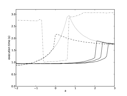
Figure 2.2. Execution time (seconds) vs truncation point, for $10^{8}$ simulations of Devroye’s algorithm (dotted line), Geweke-Robert sampler (dashed line), the inverse transform algorithm (based on the inverse transform approximation of Wichura, (1988), as implemented in the GSL library, dash-dotted line), and our algorithm (solid lines), with, from left to right, $N_{s}=1000$, $N_{s}=2000$, $N_{s}=4000$.

We implemented our algorithm, the inverse transform algorithm, Devroye’s algorithm (using cut-off value $a_{0}=0.65$) and Geweke-Robert’s algorithm in C, using the GNU Scientific library (GSL). Figure 2.2 plots the execution time of $10^{8}$ runs on a 2.8 Ghz desktop computer, for each algorithm and for different values of the truncation point $a$. Our algorithm appears to be up to two times faster than Geweke-Robert’s algorithm, and up to three times faster than Devroye’s algorithm and the inverse transform method. The three solid lines correspond to different sizes $N_{s}$, $N_{s}=1000,\,2000,\,4000$, from left to right, of the five arrays containing the constants $x_{i}$, $y_{i}$, $\underline{y}_{i}$, $d_{i}$, $\delta_{i}$; note that only those values such that $x_{i},x_{i+1}\in[a_{\min},a_{\max}]$ need to be stored, hence $N_{s}<2N$. Figure 2.2 shows that increasing $N_{s}$ only improves the execution time for a tiny interval of $a$ values, so there may be little point in increasing $N_{s}$ further than, say, $4000$. For $N_{s}=4000$, the acceptance rate is typically above $0.99$ or even $0.999$ for most values of $a\in[a_{\min},a_{\max}]$. The increase of the computational cost for $a>2$ is due to the increasing probability of sampling $X$ from the right tail using Devroye’s algorithm. Outside of the range of the represented interval, the rejection algorithms have a similar computational cost, as they perform the same operations. For $N_{s}=4000$ and a double precision implementation, the total memory cost of the algorithm is 162 kB, a small fraction of the memory cache of most modern CPU’s. (A CPU memory cache is a small, fast memory where a CPU stores data used repetitively.)

2.5. Truncation to a finite interval $[a,b]$

The extension to finite truncation intervals $[a,b]$ is straightforward. First, one determines a region index $i_{a}$ (resp. $i^{\prime}_{b}$) such that either region $i_{a}$ or region $i_{a}+1$ (resp. region $i^{\prime}_{b}$ or region $i^{\prime}_{b}-1$) contains $a$ (resp. $b$), using the table look-up method described in 2.3. Then, one proceeds as above, choosing randomly a region in the range $i_{a},\ldots,i^{\prime}_{b}$, and so on.

However, a difficulty arises if $(b-a)$ is small. Suppose for instance that $a$ and $b$ fall in the same region, and that $b-a$ is small with respect to the width of the region. Then, if one samples uniformly point $(X,Y)$ within that region, the probability that $a\leq X\leq b$ may be arbitrarily small.

We propose the following work-around: when $i_{b}^{\prime}-i_{a}\leq k_{\min}$, say $k_{\min}=5$, use instead a rejection algorithm based on Devroye, (1986)’s exponential proposal, but truncated to $[a,b]$, i.e.,

(2.4) $$q(x)=\frac{\lambda\exp(-\lambda x)}{\exp(-\lambda a)-\exp(-\lambda b)}I(a\leq x\leq b).$$

with $\lambda=a$ (resp. $\lambda=b$) when $b>0$ (resp. when $b\leq 0$). The advantage of this approach is that it gives an acceptance rate close to $1$ whatever the values of $a$, and $b$, subject to $i_{b}^{\prime}-i_{a}\leq k_{\min}$; i.e., whether $a$ and $b$ are both in the same tail, or both close to $0$. In the latter case, $q$ should be close numerically to a uniform distribution.

3. Bi-dimensional case: semi-finite intervals

We now consider the simulation of $X=(X_{1},X_{2})\sim N_{2}(\mu,\Sigma)$, subject to $X_{1}\geq a_{1}$ and $X_{2}\geq a_{2}$. Without loss of generality, we set $\mu=(0,0)^{\prime}$,

$$\Sigma=\left(\begin{array}[]{cc}1&\rho\\ \rho&1\end{array}\right),$$

and assume that $a_{1}\geq a_{2}$; if necessary, swap components to impose the last condition. The joint density of the considered truncated density is, up to a constant:

(3.1) $$p(x_{1},x_{2})\propto\exp\left\{-\frac{1}{2\nu^{2}}\left(x_{1}^{2}+x_{2}^{2}-2\rho x_{1}x_{2}\right)\right\}I\left(x_{1}\geq a_{1};x_{2}\geq a_{2}\right),$$

where the short-hand $\nu^{2}=1-\rho^{2}$ will be used throughout the rest of the paper. The conditional distribution of $X_{2}|X_{1}=x_{1}$ is a univariate Gaussian $N(\rho x_{1},\nu^{2})$ truncated to $X_{2}\geq a_{2}$, which we denote from now on $TN_{[a_{2},\infty)}(\rho x_{1},\nu^{2})$. A common misconception is that the marginal density of $X_{1}$ is also a truncated Gaussian density, although standard calculus leads to:

(3.2) $$p(x_{1})\propto\varphi(x_{1})\Phi\left(\frac{\rho x_{1}-a_{2}}{\nu}\right)I(x_{1}\geq a_{1}).$$

In order to simulate from (3.1), a natural strategy is to derive a rejection algorithm for the marginal (3.2), and to simulate $X_{2}$ conditional on $X_{1}$, using the algorithm we developed in Section 2. This is basically the approach adopted here, although we shall see that, in some cases, it is preferable to derive a rejection sampler for the joint distribution (3.1). We mention briefly that universal bivariate samplers exist, see e.g. Hörmann, (2000) or Leydold, (2000), but as in the univariate case our objective is to design a specialised algorithm that runs faster (i.e., does not require a set-up time), for situations where only one random vector must be generated.

To derive a proposal distribution for (3.2), we substitute the $\Phi(\cdot)$ factor with a simpler expression derived from the two following straightforward inequalities:

(3.3) $$\frac{1}{2}\leq\Phi(x)\leq 1\quad\mbox{for }x\geq 0,$$

(3.4) $$\Phi(x)\leq c(x_{0})\varphi(x)\quad\mbox{for }x\leq x_{0}\leq 0,$$

where $c(x_{0})=(\sqrt{\pi/2})\wedge(-1/x_{0})$, for $x_{0}<0$, $c(0)=\sqrt{\pi/2}$. We now distinguish between cases where the argument of $\Phi(\cdot)$ in (3.2) is positive, negative, or both, over the range of possible values for $x_{1}.$ We consider the following cases, and treat them separately:

• case $S^{+}$: either $\rho\geq 0$ and $\rho a_{1}-a_{2}\geq 0$, or $\rho<0$ and $a_{1}\leq\Phi^{-1}(1/3)\approx-0.4307$

• case $S^{-}$: $\rho<0$, $\rho a_{1}-a_{2}\leq 0$, and $a_{1}>\Phi^{-1}(1/3)\approx-0.4307$.

• case $M^{+}:$ $\rho\geq 0$ and $\rho a_{1}-a_{2}<0$.

• case $M^{-}$: $\rho<0$, $\rho a_{1}-a_{2}>0$, and $a_{1}>\Phi^{-1}(-1/3)\approx-0.4307$.

where ‘S’ stands for ‘Simple’, and ‘M’ for ‘Mixture’, as we elaborate below.

We now prove that, in each case, it is possible to derive a rejection algorithm with an acceptance rate bounded from below for all values of $\rho$, $a_{1}$ and $a_{2}$.

3.1. Case $S^{+}$

Assuming first $\rho\geq 0$ and $\rho a_{1}-a_{2}\geq 0$, then, according to (3.3),

(3.5) $$\Phi\left(\frac{\rho x_{1}-a_{2}}{\nu}\right)\in[1/2,1]$$

for all $x\geq a_{1},$ which suggests the following proposal distribution:

$$q_{S^{+}}(x_{1})\propto\varphi(x_{1})I(x_{1}\geq a_{1}),$$

i.e., a $TN_{[a_{1},+\infty)}(0,1)$ distribution, in order to sample from the marginal $p(x_{1})$. For a given $x_{1}$ simulated from $q_{S^{+}}$, the acceptance probability equals (3.5), hence the acceptance rate of such a rejection algorithm equals

(3.6) $$\int_{a_{1}}^{+\infty}\Phi\left(\frac{\rho x_{1}-a_{2}}{\nu}\right)\frac{\varphi(x_{1})}{\Phi(-a_{1})}\,dx_{1},$$

and is larger than $1/2$ by construction.

However, it is more efficient to simulate jointly $(X_{1},X_{2})$ as follows: sample $X_{1}\sim TN_{[a_{1},\infty)}(0,1)$, $X_{2}|X_{1}=x_{1}\sim N(\rho x_{1},\nu^{2})$, and accept if $X_{2}\geq a_{2}$; otherwise repeat. It is easy to check that the latter rejection algorithm has exactly the same acceptance rate, i.e., (3.6), as the former, but it is faster, because it does not perform any evaluation of $\Phi$, and because $X_{2}$ is obtained ‘for free’, i.e., a second step is not required to generate $X_{2}$.

When $\rho<0$, the argument of $\Phi$ in (3.6) is not positive for all $x_{1}\geq a_{1}$, but the integral is still larger than $1/2$ provided $a_{1}\leq\Phi^{-1}(1/3)$. To establish this property, one may remark that (3.6) is the probability that $X_{2}\geq a_{2}$, conditional on $X_{1}\geq a_{1}$, provided $(X_{1},X_{2})\sim N_{2}(\mu,\Sigma)$. This probability decreases with respect to $a_{2}$, $a_{2}\leq a_{1}$, and, for $a_{2}=a_{1}$, this probability decreases with respect to $-\rho$ and $a_{1}$. Finally, for $\rho=-1$ and $a_{1}=a_{2}=\Phi^{-1}(1/3)$, this probability equals $1/2.$ Thus, we use Algorithm $S^{+}$ also when $\rho<0$ and $a_{1}\leq\Phi^{-1}(1/3)$.

3.2. Case $S^{-}$

If $\rho<0$ and $\rho a_{1}-a_{2}\leq 0$, then inequality (3.4) holds for all values of the argument $x=(\rho x_{1}-a_{2})/\nu$, and for $x_{0}=(\rho a_{1}-a_{2})/\nu$. This suggests the following algorithm: sample $X_{1}$ from proposal density

$$q_{S^{-}}(x_{1}) \propto \varphi(x_{1})\varphi\left(\frac{\rho x_{1}-a_{2}}{\nu}\right)I(x_{1}\geq a_{1})$$

$$\propto \varphi\left(x_{1};\rho a_{2},\nu^{2}\right)I(x_{1}\geq a_{1})$$

that is, the density of truncated Gaussian distribution $TN_{[a_{1},\infty)}(\rho a_{2},\nu^{2})$, and accept with probability:

(3.7) $$\psi\left(-\frac{\rho x_{1}-a_{2}}{\nu}\right)/c\left(\frac{\rho a_{1}-a_{2}}{\nu}\right),$$

where $\psi(x)=\Phi(-x)/\varphi(x)$. The acceptance rate is then:

(3.8) $$E_{TN_{[a_{1},\infty)}(\rho a_{2},\nu^{2})}\left[\psi\left(-\frac{\rho X_{1}-a_{2}}{\nu}\right)\right]/c\left(\frac{\rho a_{1}-a_{2}}{\nu}\right).$$

We show formally in Appendix B1 that this acceptance rate admits a lower bound which is larger than $0.416$; our numerical studies indicate that the optimal lower bound may be $1/2$. Intuitively, the idea behind inequality (3.4) is that $\Phi(-x)\approx\varphi(x)/x$ for large values of $x$, hence the true marginal density $p(x_{1})$ behaves like a Gaussian density density times $1/(a_{2}-\rho x_{1})$, but the latter factor varies slowly with respect to a Gaussian density, so it can be discarded in the proposal.

3.3. Case $M^{-}$

If $\rho<0$ and $\rho a_{1}-a_{2}>0$, the quantity $(\rho x_{1}-a_{2})/\nu$ takes positive and negative values for $x_{1}\geq a_{1}$. To combine both inequalities, one may use a mixture proposal:

(3.9) $$q_{M^{-}}(x_{1})\propto\varphi(x_{1})I\left(\rho x_{1}-a_{2}>0\right)+\sqrt{\frac{\pi}{2}}\varphi(x_{1})\varphi\left(\frac{\rho x_{1}-a_{2}}{\nu}\right)I\left(\rho x_{1}-a_{2}<0\right)$$

subject to $x_{1}\geq a_{1}$. To sample from the mixture proposal, choose component $1$ (corresponding to the first term above), with probability $\omega_{1}/(\omega_{1}+\omega_{2})$, with

$$\omega_{1}=\Phi(a_{2}/\rho)-\Phi(a_{1})$$

$$\omega_{2}=\frac{\nu}{2}\exp\left\{-\frac{a_{2}^{2}}{2}\right\}\Phi\left(-\frac{a_{2}\nu}{\rho}\right)$$

and choose component 2 otherwise. If component 1 is chosen, one can use the same shortcut as in Algorithm $S^{+}$, that is, draw $X_{1}\sim TN_{[a_{1},a_{2}/\rho]}(0,1)$ and $X_{2}|X_{1}=x_{1}\sim N(\rho x_{1},\nu^{2})$, and accept the simulated pair $(x_{1},x_{2})$ if $x_{2}\geq a_{2}$. If component 2 is chosen, the proposed value for $X_{1}$ is drawn from a $TN_{[a_{2}/\rho,\infty)}(\rho a_{2},\nu^{2})$ distribution, and is accepted with probability

$$\sqrt{\frac{2}{\pi}}\psi\left(-\frac{\rho x_{1}-a_{2}}{\nu}\right).$$

When a draw $x_{1}$ is accepted, it is completed with $x_{2}$ drawn from $X_{2}|X_{1}=x_{1}\sim TN_{[a_{2},+\infty)}(\rho x_{1},\nu^{2})$.

The acceptance rate of this algorithm is a weighted average (with weights given by $\omega_{1}$ and $\omega_{2}$) of the acceptance rate of Component 1, which is larger than $1/2$ by construction, and the acceptance rate of algorithm $S^{-}$ for $a_{2}=\rho a_{1}$, which is also bounded from below, as explained in the previous subsection.

3.4. Case $M^{+}$

If $\rho\geq 0$ and $\rho a_{1}-a_{2}\leq 0$, then again $(\rho x_{1}-a_{2})/\nu$ take both negative and positive values for $x_{1}\geq a_{1}$, which suggests that we use a mixture proposal similar to (3.9). Unfortunately, the acceptance rate may be arbitrarily small in that case. Exact calculations are omitted for the sake of space, but it can be shown that the mode of $p(x_{1})$ can be arbitrary far from $x_{1}=a_{2}/\rho$, the point where the two components intersect, which gives an arbitrary small acceptance rate.

Instead, we substitute (3.4) with a slightly different inequality:

(3.10) $$\Phi(x)\leq d(x_{0})\varphi(x)e^{\lambda x}\quad\mbox{for }x_{0}\leq x\leq 0$$

where $\lambda=0.68$, $d(x_{0})=(\sqrt{\pi/2})\vee\chi(-x_{0})$, and $\chi(x)=e^{\lambda x}\Phi(-x)/\varphi(x)$. This inequality stems from straightforward calculus. Other values of $\lambda$ are also valid, but in our numerical experiments, $\lambda=0.68$ seemed to be close to optimal, in terms of minimum acceptance rate.

This inequality leads to the following proposal mixture density:

$$q_{M^{+}}(x_{1}) \propto \varphi(x_{1})I\left(\rho x_{1}-a_{2}\geq 0\right)$$

$$+\varphi(x_{1})\varphi\left(\frac{\rho x_{1}-a_{2}}{\nu}\right)\exp\left(\frac{\lambda(\rho x_{1}-a_{2})}{\nu}\right)d\left(\frac{\rho a_{1}-a_{2}}{\nu}\right)I\left(\rho x_{1}-a_{2}<0\right)$$

subject to $x_{1}\geq a_{1}$. The second term is proportional to a $N(\theta,\nu^{2})$ density, with $\theta=\rho(a_{2}+\lambda\nu)$. To sample from this mixture, choose component $1$, with probability $\tau_{1}/(\tau_{1}+\tau_{2})$, choose component 2 otherwise, where

$$\tau_{1}=\Phi(-a_{2}/\rho)$$

$$\tau_{2} = \frac{\nu}{\sqrt{2\pi}}\left\{\Phi\left(\frac{a_{2}/\rho-\theta}{\nu}\right)-\Phi\left(\frac{a_{1}-\theta}{\nu}\right)\right\}$$

$$\qquad\exp\left\{\frac{\theta^{2}-a_{2}^{2}-2\lambda\nu a_{2}}{2\nu^{2}}\right\}d\left(\frac{\rho a_{1}-a_{2}}{\nu}\right).$$

If component 1 is selected, draw $X_{1}\sim TN_{[a_{2}/\rho,+\infty)}(0,1)$, $X_{2}|X_{1}=x_{1}\sim N(\rho x_{1},\nu^{2})$, and accept simulated pair $(x_{1},x_{2})$ if $x_{2}\geq a_{2}$. Otherwise, draw $X_{1}\sim TN_{[a_{1},a_{2}/\rho]}(\theta,\nu^{2})$, and accept with probability

$$\chi\left(\frac{a_{2}-\rho x_{1}}{\nu}\right)/d\left(\frac{a_{2}-\rho a_{1}}{\nu}\right),$$

and, upon acceptance, complete with

$$X_{2}|X_{1}=x_{1}\sim TN_{[a_{2},+\infty)}(\rho x_{1},\nu^{2}).$$

We show formally in Appendix B2 that the acceptance rate of this algorithm is bounded from below by $0.22$, and we found numerically that the optimal lower bound seems to be $1/2$, see Section 3.6.

3.5. Computational cost

The above algorithms, except algorithm $S^{+}$, involve a few evaluations of function $\Phi$, which is expensive. But such evaluations can be bypassed in most cases. In algorithm $S^{-}$ for instance, given the expression of acceptance probability (3.7), one should accept the proposed value $x_{1}$ if and only if

$$\Phi\left(rx_{1}+s\right)\geq ut(x_{1})$$

where $u$ is an uniform variate, and the exact expression of $r,$ $s$, and $t$ are easily deduced from (3.7). If good, fast approximations of $\Phi$ are available, such that $\underline{\Phi}(x)\leq\Phi(x)\leq\overline{\Phi}(x)$, it is enough to check that $\underline{\Phi}\left(rx_{1}+s\right)\geq ut(x_{1})$ (resp. $\overline{\Phi}\left(rx_{1}+s\right)<ut(x_{1})$) to accept (resp. reject) $x_{1}$. It is only when $ut(x_{1})$ is very close to $\Phi\left(rx_{1}+s\right)$ that an exact evaluation of $\Phi\left(rx_{1}+s\right)$ is required.

Such fast, good approximations of $\Phi$ may be deduced from the tables of our univariate algorithm, see Section 2.3. Specifically, and using the same notations as Section 2.3, let $z=rx_{1}+s$, and assume that $z\in[a_{\min},a_{\max}]$, then one may set $\overline{\Phi}(z)=A(j_{\left\lfloor z/h\right\rfloor}+1)$, where $A(i)>\Phi(x_{i+1})$ denotes the total area of all the regions up to region $i$, and may be computed beforehand and hard-coded in the program like the other constants $y_{i}$, $d_{i}$ and so on. One may define similarly $\underline{\Phi}(z)$ using $\Phi(z)=1-\Phi(-z)$. When $z\notin[a_{\max},a_{\min}]$, one may use the expansion of Abramowitz and Stegun, (1965, p. 932) to derive the following upper and lower approximations

$$\overline{\Phi}(z)=-\frac{\varphi(z)}{z}\left\{1-\frac{1}{z^{2}}+\frac{3}{z^{4}}\right\},\qquad\underline{\Phi}(z)=-\frac{\varphi(z)}{z}\left\{1-\frac{1}{z^{2}}+\frac{3}{z^{4}}-\frac{15}{z^{6}}\right\},$$

for $z<0$. (For $z>0$, similar formulae are obtained using $\Phi(z)=1-\Phi(-z$)). Note also that one does not necessarily have to compute all the terms of these expressions. For instance, if $\overline{\Phi}_{1}(\alpha x_{1}+\beta)<u\upsilon(x_{1})$, where $\overline{\Phi}_{1}(z)=-\varphi(z)/z$, then the proposed value can be rejected without computing the remaining terms. This principle can be used for each term of the expansion, but, on the other hand, it is preferable not to expand further the expressions above, since they work well already for reasonable values of $a_{\min}$ and $a_{\max}$, and since that would define diverging series.

Provided the above strategy is implemented, the algorithms proposed in the section are reasonably fast, since they only involve a few basic operations, and their acceptance rate is greater than $1/2$ for all parameters. Algorithms $M^{+}$ and $M^{-}$ are slightly more expensive, as they require sampling a mixture index, but note that the same strategy can be implemented in order to avoid with good probability the evaluation of functions $\Phi$ appearing in the expression of the mixture weights.

3.6. Numerical illustration

We simulated $10^{5}$ parameters $(a_{1},a_{2},\rho)$, where $\rho\sim U[-1,1]$, $a_{1}$, $a_{2}\sim N(0,s^{2})$, conditional on $a_{1}\geq a_{2}$. For each parameter, we evaluated the acceptance rate of our algorithm by computing the average acceptance probability over the proposed draws generated by $1000$ runs. Figure 3.1 reports the histogram of the acceptance rates for $s=1$; larger values of $s$ give histograms that are even more concentrated around $1$.

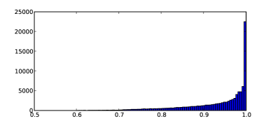
Figure 3.1. Histogram of acceptance rates corresponding to $10^{5}$ simulated vectors $(a_{1},a_{2},\rho)$, where $\rho\sim U[0,1]$, $a_{1}$, $a_{2}\sim N(0,1)$, conditional on $a_{1}\geq a_{2}$.

In this simulation exercise, $90\%$ of the acceptance rates are above $0.8$ and $99\%$ are above $0.65$; none is lower than $1/2$.

4. Bi-dimensional case: finite intervals

We now consider the simulation of $X=(X_{1},X_{2})\sim N_{2}(0,\Sigma)$, with

$$\Sigma=\left(\begin{array}[]{cc}1&\rho\\ \rho&1\end{array}\right),$$

conditional on $X_{1}\in[a_{1},b_{1}]$ and $X_{2}\in[a_{2},b_{2}]$, where, without loss of generality, $\rho\geq 0$. As in the previous section, the main difficulty is to sample from the marginal density of $X_{1}$:

(4.1) $$p(x_{1})\propto\varphi(x_{1})\left[\Phi(\alpha x_{1}+\beta_{1})-\Phi(\alpha x_{1}+\beta_{0})\right]I(a_{1}\leq x_{1}\leq b_{1})$$

where $\alpha=\rho/\nu\geq 0$, $\beta_{1}=-a_{2}/\nu$, $\beta_{0}=-b_{2}/\nu$ and $\beta_{1}\geq\beta_{0}$, since the distribution of $X_{2}$ conditional on $X_{1}=x_{1}$ is the univariate truncated Gaussian distribution $TN_{[a_{2},b_{2}]}(\rho x_{1},\nu^{2})$.

We shall consider two situations, according to whether $\beta_{1}-\beta_{0}<\Delta$ or not; we take $\Delta=2$, which seems to close to the optimal value in our simulations, in terms of minimum acceptance rate.

When $\beta_{1}-\beta_{0}$ is small (case $T$), one may Taylor expand the second factor of (4.1), which is denoted $\kappa$ from now on, into:

$$\kappa(x_{1})=\Phi(\alpha x_{1}+\beta_{1})-\Phi(\alpha x_{1}+\beta_{0})\approx(\beta_{1}-\beta_{0})\varphi\left(\alpha x_{1}+\frac{\beta_{0}+\beta_{1}}{2}\right),$$

hence $\kappa$ behaves like a Gaussian density, see the right panel of Figure 4.1. Therefore, $p(x_{1})$ is also well approximated by a Gaussian, which is the basis of algorithm T detailed in 4.2.

Otherwise, when $\beta_{1}-\beta_{0}$ is large, $\kappa$ behaves like the curve plotted in the left panel of Figure 4.1. In this case, called $M^{3}$ below, we cut $\kappa$ into at most three pieces, and derive a mixture proposal, using ideas similar to the previous section.

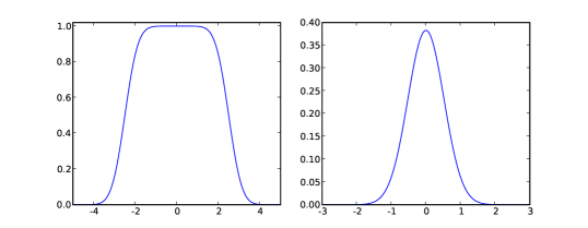
Figure 4.1. Function $\kappa(x_{1})=\Phi(\alpha x_{1}+\beta_{1})-\Phi(\alpha x_{1}+\beta_{0})$ , for $(\alpha,\beta_{0},\beta_{1})=(2,-5,5)$ (left), and $(\alpha,\beta_{0},\beta_{1})=(2,-0.5,0.5)$ (right)

4.1. Case $M^{3}$

Let $\gamma_{i}=-\beta_{i}/\alpha$, for $i=0,1$, and $\upsilon=(\beta_{1}-\beta_{0})/2$; note $\gamma_{1}\leq\gamma_{0}$ since $\beta_{0}\leq\beta_{1}$. We may divide the curve of $\kappa$ into three parts, so as to re-use the same ideas as in Section 3, that is, deriving a mixture of Gaussian proposals. Specifically,

• for $x_{1}<\gamma_{1}$, one shows easily that

  $$\left\{2\Phi(\Delta)-1\right\}\Phi(\alpha x_{1}+\beta_{1})\leq\kappa(x_{1})\leq\Phi(\alpha x_{1}+\beta_{1}).$$

  We know already that target density $\varphi(x_{1})\Phi(\alpha x_{1}+\beta_{1})I(x_{1}<\gamma_{1})$ can be simulated efficiently using a particular Gaussian proposal density, see Component 2 of Algorithm $M^{+}$ in Section 3.4. The above inequality indicates that, using the same proposal, one should obtain an acceptance rate which is at least $2\Phi(\Delta)-1$ times the minimum acceptance rate of $M^{+}$, that is, $\Phi(\Delta)-1/2\approx 0.477.$

• for $x_{1}\in[\gamma_{1},\gamma_{0}]$, $\kappa$ is roughly flat, and

  $$\Phi(\Delta)-1/2\leq\kappa(x_{1})\leq 2\Phi(\upsilon)-1\leq 1.$$

  This suggests using proposal distribution $X_{1}\sim TN_{[\gamma_{1}\vee a_{1},\gamma_{0}\wedge b_{1}]}(0,1)$, and accept realisation $x_{1}$ with probability $\kappa(x_{1})/\left\{2\Phi(\upsilon)-1\right\}$. The acceptance probability is then bounded from below by $\Phi(\Delta)-1/2\approx 0.477$.

• for $x_{1}>\gamma_{0}$, one has:

  $$\left\{2\Phi(\Delta)-1\right\}\Phi(-\alpha x_{1}-\beta_{0})\leq\kappa(x_{1})\leq\Phi(-\alpha x_{1}-\beta_{0}).$$

  Again, one may use the same proposal as for Component 2 of algorithm $M^{-}$ , see 3.3, which should lead to an acceptance rate which is larger than $\Phi(\Delta)-1/2\approx 0.477$.

The principle of Algorithm $M^{3}$ is therefore to draw from a mixture of at most three components, the relative weights of which are given below, and given the chosen component, to use one of the three strategies described above.

Denote $\zeta_{l}$, $\zeta_{c}$, $\zeta_{r}$, the unnormalised weights of the left, centre, and right components, respectively. In case $b_{1}\vee\gamma_{1}>0$, one has

$$\zeta_{l}=\frac{\nu\,d(\alpha a_{1}+\beta_{1})}{\sqrt{2\pi}}\exp\left(\frac{m_{l}^{2}-a_{2}^{2}-2\lambda\nu a_{2}}{2\nu^{2}}\right)\left\{\Phi\left(\frac{\gamma_{1}-m_{l}}{\nu}\right)-\Phi\left(\frac{a_{1}-m_{l}}{\nu}\right)\right\}I(\gamma_{1}\geq a_{1})$$

with $m_{l}=\rho(a_{2}+\lambda\nu)$ and function $d$ was defined in Section 3.4; Otherwise, one obtains the same expression, but with $\lambda$ set to $0$, i.e.,

$$\zeta_{l}=\frac{\nu}{2}\exp\left(-\frac{a_{2}^{2}}{2}\right)\left\{\Phi\left(\frac{\gamma_{1}-m_{l}}{\nu}\right)-\Phi\left(\frac{a_{1}-m_{l}}{\nu}\right)\right\}I(\gamma_{1}\geq a_{1})$$

with $m_{l}=\rho a_{2}$. In all cases,

$$\zeta_{c}=\left\{2\Phi(\upsilon)-1\right\}\left\{\Phi(\gamma_{0}\wedge b_{1})-\Phi(\gamma_{1}\vee a_{1})\right\}I(b_{1}>\gamma_{1};a_{1}<\gamma_{0}),$$

$$\zeta_{r}=\frac{\nu}{2}\exp\left(-\frac{b_{2}^{2}}{2}\right)\left\{\Phi\left(\frac{b_{1}-\rho b_{2}}{\nu}\right)-\Phi\left(\frac{\gamma_{0}-\rho b_{2}}{\nu}\right)\right\}I(b_{1}>\gamma_{0}).$$

One may show that the acceptance rate of this algorithm is bounded from below by $1/2-\Phi(-\Delta)\approx 0.477$; simulations suggest this bound is optimal. We omit the exact calculations, as they are similar to those of previous algorithms. We managed to obtain this result under the following assumptions: (i) $\rho\geq 0$; (ii) $b_{2}\geq 0$ and (iii) either $a_{2}\geq a_{1}$ or $b_{1}\leq 0$. It is always possible to enforce such conditions, by either swapping $X_{1}$ and $X_{2}$, or changing their signs, or both. We note also that, in most of our simulated exercises, at least one component of this mixture is empty, and often two of them are, which makes it possible to skip calculating the weights and simulating the mixture index.

4.2. Case $T$

As explained above, when $\beta_{1}-\beta_{0}<\Delta$, a good Gaussian approximation of $p(x_{1})$ is

$$q(x_{1})\propto\varphi(x_{1})\varphi\left(\alpha x_{1}+\frac{\beta_{0}+\beta_{1}}{2}\right)$$

that is, a $N(m,s^{2})$ density with

$$(m,s^{2})=\left(-\frac{\alpha(\beta_{0}+\beta_{1})}{2(1+\alpha^{2})},\frac{1}{1+\alpha^{2}}\right).$$

In our experiments, this approximation appears to be accurate for all values of $\alpha$, $\beta_{0}$, $\beta_{1}$ (in the sense that the rejection rate of the algorithm we now describe is always larger than 0.47 in our simulations, see next subsection). On the other hand, it seems difficult to apply approximations similar to those we used before. Instead, we note that $p(x_{1})$ is a log-concave density (Prekopa,, 1973). This suggests using either exponential or piecewise exponential proposals, and working out a simplified version of ARS (Adaptive Rejection Sampling, Gilks and Wild,, 1992).

Specifically, let $\xi$ denote the marginal log-density of $X_{1}$:

$$\xi(x_{1})=\log\varphi(x_{1})+\log\kappa(x_{1})$$

the derivative of which is easy to compute:

$$\xi^{\prime}(x_{1})=-x_{1}+\alpha\frac{\varphi(\alpha x_{1}+\beta_{1})-\varphi(\alpha x_{1}+\beta_{0})}{\Phi(\alpha x_{1}+\beta_{1})-\Phi(\alpha x_{1}+\beta_{0})},$$

which leads to the inequality

$$\xi(x_{1})\leq\xi(v)+\xi^{\prime}(v)(x_{1}-v)$$

for any $x_{1},v\in[a_{1},b_{1}]$. Up to a constant, the right hand side is the log-density of the truncated Exponential distribution $\mathrm{Exp}_{[a_{1},b_{1}]}(\lambda)$ defined in (2.4), with $\lambda=\xi^{\prime}(v)$; note that $\lambda$ may be negative. Thus, one may sample $x{}_{1}\sim\mathrm{Exp}_{[a_{1},b_{1}]}\left\{\xi^{\prime}(v)\right\}$, and accept with probability

$$\exp\left\{\xi(x_{1})-\xi(v)-\xi^{\prime}(v)(x_{1}-v)\right\}.$$

Obviously, the difficulty is to choose $v$. Since the target density is well approximated by a $TN_{[a_{1},b_{1}]}(m,s^{2})$, and assuming that $a_{1}\geq m$ (resp. $b_{1}\leq m$), it seems reasonable to set $v=(m+s)\vee a_{1}$ (resp. $v=(m-s)\wedge b_{1}$). These values would be optimal if the target density would be equal to its approximation $TN_{[a_{1},b_{1}]}(m,s^{2})$. In case $a_{1}<m$ and $b_{1}>m$, i.e., the mean $m$ is within $[a_{1},b_{1}]$, we use instead a mixture proposal, based on two well chosen points $v,w\in[a_{1},b_{1}]$, say $v<w$. Thus,

$$\xi(x_{1})\leq\left\{\xi(v)+\xi^{\prime}(v)(x_{1}-v)\right\}\wedge\left\{\xi(w)+\xi^{\prime}(w)(x_{1}-w)\right\}$$

and one may sample from the density defined as the exponential of the right hand side above (which is a piecewise exponential distribution), and accept with probability

$$\exp\left[\xi(x_{1})-\left\{\xi(v)+\xi^{\prime}(v)(x_{1}-v)\right\}\wedge\left\{\xi(w)+\xi^{\prime}(w)(x_{1}-w)\right\}\right].$$

Note that, in the original ARS algorithm of Gilks and Wild, (1992), the proposal is progressively refined by adding a new component each time the proposed value is rejected. We found however that the acceptance rate of Algorithm T described above is generally above $1/2$, so using fixed proposals with at most two components seems reasonable. Obviously, the good properties of the above algorithm lie in the good choice of points $v$, $w$, which was made possible by the knowledge of a good approximation of the target density.

We were not able to prove formally that the acceptance rate of Algorithm T is bounded from below, as in previous cases, so we performed intensive simulations for assessing its properties; the acceptance rate of Algorithm T seems to converges to one for limiting values, say $a_{1}\rightarrow-\infty$ but with $b_{1}-a_{1}$ and $\rho$ kept fixed; and to be bounded from below by $1/2.$

4.3. Numerical illustration

We simulated $10^{5}$ parameters $(a_{1},b_{1},a_{2},b_{2},\rho)$, where $\rho\sim U[-1,1]$, $a_{1}$, $a_{2}\sim N(0,2^{2})$, and $b_{i}=a_{i}+2e_{i}$ with $e_{i}\sim\mathrm{Exp}(1)$, $i=1,2$. For each parameter, we evaluated the acceptance rate of our algorithm by computing the average acceptance probability over the proposed draws generated by $1000$ runs. Figure 4.2 reports the histogram of the acceptance rates. About $90\%$ of these values are above $0.71$, about $99\%$ are above $0.55$, and all values are above $0.47$, as expected.

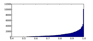
Figure 4.2. Histogram of acceptance rates for $10^{5}$ simulated parameters $(\rho,a_{1},b_{1},a_{2},b_{2})$, with $\rho\sim U[-1,1]$, $a_{1}$, $a_{2}\sim N(0,2^{2})$, and $b_{i}=a_{i}+2e_{i}$ with $e_{i}\sim\mathrm{Exp}(1)$, $i=1,2.$

5. Generalisation to 3 or more dimensions

We discuss briefly the problem of simulating $d$-dimensional truncated Gaussian distributions, for $d\geq 3$ and for semi-finite truncation intervals; i.e., $X\sim N_{d}(0_{d},\Sigma)$, subject to $X_{i}\geq a_{i}$, $i=1,\ldots,d$. As we have done for $d=2$, we assume without loss of generality that $a_{1}\geq\ldots\geq a_{d}$. It does not seem possible to generalise to dimension $d\geq 3$ algorithms based on mixture proposals, i.e., $M^{+}$ and $M^{-}$, as the corresponding mixture weights would involve intractable integrals. But algorithms $S^{+}$ and $S^{-}$ can be generalised to larger dimensions, as explained below, which makes it possible to sample $X$ under certain conditions on $\Sigma$ and $a=(a_{1},\ldots,a_{d}$).

5.1. Extension of Algorithm $S^{+}$

An obvious way of generalising Algorithm $S^{+}$ to 3 dimensions is to do the following. Let $Q=(q_{ij})=\Sigma^{-1}$ and $\Sigma_{12}$ denote the sub-matrix obtained by removing the last row and the last column from $\Sigma$, then:

1. Sample $(X_{1},X_{2})\sim N_{2}(0_{2},\Sigma_{12})$ conditional on $X_{1}\geq a_{1}$ and $X_{2}\geq a_{2}$ (using one of the algorithms discussed in Section 3)

2. Sample from the unconstrained conditional distribution of $X_{3}$:

   $$X_{3}|\left\{X_{1}=x_{1},X_{2}=x_{2}\right\}\sim N\left(-\frac{q_{13}x_{1}+q_{23}x_{2}}{q_{33}},\frac{1}{q_{33}}\right)$$

3. If $x_{3}\geq a_{3}$, accept the simulated vector $(x_{1},x_{2},x_{3})$; otherwise reject and go to Step 1.

One easily shows that the acceptance rate corresponding to Step 3 is larger than $1/2$ under the following set of conditions: $q_{13}\leq 0$, $q_{23}\leq 0$ and $q_{13}a_{1}+q_{23}a_{2}+q_{33}a_{3}\leq 0$.

One may iterate the above principle so as to extend Algorithm $S^{+}$ to any dimension $d$; i.e., for $d=4$, add Step 4 where $X_{4}$ is simulated from the appropriate conditional distribution and accept if $X_{4}\geq a_{4}$; provided appropriate conditions similar to those above, are iteratively verified, one obtains an overall acceptance rate that is at least $2^{-(d-1)}$, since each rejection step (including Step 1 above for the first two variates $X_{1}$ and $X_{2}$) induces an acceptance rate that is at least $1/2$.

We note that these iterative conditions imply in particular that any pair of components of $X$ is positively correlated, except for $(X_{1},X_{2})$ which may have any type of correlation. There are several practical settings where this assumption is met, such as in Gaussian Markov random fields models (e.g. Rue and Held,, 2005) where one would impose positive correlation between neighbour nodes. Thus, in such or other particular settings, and since the acceptance rate is expected to be higher than its lower bound for most parameters, as observed in two dimensions, the above algorithm may remain practical for dimensions as large as 4 or 5. For instance, in a Markov chain Monte Carlo context involving truncated Gaussian vectors or large dimension, one may try to form a larger and larger block, by including one variable at a time, checking the recursive assumptions above, and stop when either they are no longer met or the acceptance rate is too small.

5.2. Extension of Algorithm $S^{-}$

Again, assuming $d=3$, one notes that the marginal distribution of $(X_{1},X_{2})$ is:

$$p(x_{1},x_{2})\propto\exp\left\{-\frac{1}{2}\sum_{i,j=1}^{2}q_{ij}x_{i}x_{j}\right\}\Phi\left(-\frac{\sum_{i=1}^{2}q_{i3}x_{i}+q_{33}a_{3}}{q_{33}^{1/2}}\right)I\left(x_{1}\geq a_{1};x_{2}\geq a_{2}\right)$$

which suggests the following bivariate truncated Gaussian density as a proposal density:

$$p(x_{1},x_{2})\propto\exp\left\{-\frac{1}{2}\sum_{i,j=1}^{2}q_{ij}x_{i}x_{j}-\frac{\left(\sum_{i=1}^{2}q_{i3}x_{i}+q_{33}a_{3}\right)^{2}}{2q_{33}}\right\}I\left(x_{1}\geq a_{1};x_{2}\geq a_{2}\right)$$

based on inequality (3.4). For given $x_{1}$ and $x_{2}$, the acceptance probability is therefore:

$$\psi\left(\frac{\sum_{i=1}^{2}q_{i3}x_{i}+q_{33}a_{3}}{q_{33}^{1/2}}\right)/c\left(\frac{\sum_{i=1}^{2}q_{i3}x_{i}+q_{33}a_{3}}{q_{33}^{1/2}}\right)$$

where we recall that $\psi(x)=\Phi(-x)/\varphi(x)$. Using the same type of calculations as in Section 3.4, one may show that the expectation of the acceptance probability above is larger than or equal to $1/2$ provided $q_{13}\geq 0$, $q_{23}\geq 0$, and $q_{13}a_{1}+q_{23}a_{2}+q_{33}a_{3}\geq 0$. Again, this means that the overall acceptance rate is larger than or equal to $1/4$.

As in the previous section, one may iterate the construction above, so as to obtain a simulation algorithm for any dimension $d$, the acceptance rate of which is bounded from below by $2^{-(d-1)}$. This requires checking recursively conditions similar to those above. The same remarks in the previous subsection relative to the applicability of this algorithm may be repeated here.

6. Conclusion

We focused in this paper on the simulation of independent truncated Gaussian variables, but similar ideas can be used in other settings, such as importance sampling or MCMC. For instance, in case $T$, see Section 4.2, one may use the derived Gaussian approximation as an importance distribution, rather than a basis of an ARS algorithm. The same remark applies to most of our algorithms.

As briefly mentioned in the previous section, if one needs to simulate a vector from a high-dimensional truncated Gaussian distribution using MCMC, one may ask how to choose blocks of two or more variables, which will be updated using the algorithms proposed in this paper, in a way that ensures good MCMC convergence properties. A good strategy would be to form a first block of two variables with strong (conditional) correlation, then to see if additional variables may be included in that block, using the conditions given in the previous section, and repeat this process until all variables are included in a block of at least two variables. But more research is required to find the best trade-off in terms of convenience and efficiency.

Open source programs implementing the proposed algorithms are available at the author’s personal page on the website of his institution, www.crest.fr.

Appendix A: Outline of the univariate algorithm for a semi-finite truncation interval

Note Devroye($a$) refers to Devroye’s algorithm, Direct($a$) refers to the rejection algorithm based on the non truncated Gaussian distribution, see Section 2.1 for details. In both cases the input $a$ is the truncation point. Pre-computed constants consist of five floating-point tables: $(x_{i}),$ $(y_{i})$, $(\underline{y}_{i})$, $(d_{i})$ and $(\delta_{i})$; one integer table: $(j_{k})$, plus two design parameters $a_{\min}$, and $a_{\max}$.

0:  $a$ {truncation point}

0:  $x$ {simulated value}

  if $a<a_{\min}$ then

     return  Direct($a$)

  else if $a>a_{\max}$ then

     return  Devroye($a$)

  end if

  $i_{a}\leftarrow j_{\left\lfloor a/h\right\rfloor}$

  loop

     Sample integer $i$ uniformly between $i_{a}$ and $N$

     if $i=N$ then {rightmost region}

        return  Devroye($x_{N}$)

     else if $i\leq i_{a}+1$ then {two leftmost regions}

        Sample $u\sim U[0,1]$

        $x=x_{i}+d_{i}*u$

        if $x\geq a$ then

           Sample $v\sim U[0,1]$

           $y\leftarrow y_{i}*v$

           if $y\leq\underline{y}_{i}$ then

              return  $x$

           else if $y\leq\varphi(x)$ then

              return  $x$

           end if

        end if

     else {all the other regions}

        Sample $u\sim U[0,1]$

        $y\leftarrow u*y_{i}$

        if $y\leq\underline{y}_{i}$ then {occurs with high probability}

           return  $x_{i}+u*\delta_{i}$

        else

           Sample $v\sim U[0,1]$

           $x\leftarrow x_{i}+d_{i}*v$

           if $y\leq\varphi(x)$ then

              return  $x$

           end if

        end if

     end if

  end loop

Appendix B: Lower bounds for Acceptance rates

B1. algorithm $S^{-}$

Let $A(a_{1},a_{2},\rho)$ the acceptance rate (3.8), which we rewrite as:

$$A(a_{1},a_{2},\rho)=E_{TN_{[\alpha,\infty)}(\beta,\rho^{2})}\left[\psi\left(Z\right)\right]/c\left(-\alpha\right)$$

where $Z=-(\rho X_{1}-a_{2})/\nu\sim TN_{[\alpha,\infty)}(\beta,\rho^{2})$, $\alpha=(a_{2}-\rho a_{1})/\nu$, and $\beta=a_{2}\nu$. Note that $\alpha\geq 0$, $\beta\leq\alpha$, and $\psi$ is a decreasing function. Thus, the quantity above is a decreasing function of $\beta$. (To see this, one can rewrite the distribution of $Z$ as

$$Z=\beta+\rho\Phi^{-1}\left(U+(1-U)\Phi(\frac{\alpha-\beta}{\rho})\right)$$

where $U$ is an uniform variate, and check that, conditional on $U=u$, $Z$ is a decreasing function of $\beta$.). Thus, the above quantity is larger than or equal to the same quantity, but with $\beta=\alpha$:

$$A(a_{1},a_{2},\rho)\geq E_{TN_{[\alpha,\infty)}(\alpha,\rho^{2})}\left[\psi\left(Z\right)\right]/c\left(-\alpha\right)=E_{TN_{[0,\infty)}(0,1)}\left[\psi\left(\rho Z^{\prime}+\alpha\right)\right]/c\left(-\alpha\right)$$

which is a decreasing function of $\rho,$ hence

(6.1) $$A(a_{1},a_{2},\rho)\geq E_{TN_{[0,\infty)}(0,1)}\left[\psi\left(Z^{\prime}+\alpha\right)\right]/c\left(-\alpha\right),$$

and since $c(-\alpha)=(\sqrt{\pi/2})\wedge(1/\alpha)$, one can show that the bound is minimised for $\alpha=\sqrt{\pi/2}$, which leads to:

$$A(a_{1},a_{2},\rho)\geq\sqrt{\frac{2}{\pi}}E_{TN_{[0,\infty)}(0,1)}\left[\psi\left(Z^{\prime}+\sqrt{\frac{2}{\pi}}\right)\right]\approx 0.416.$$

This lower bound is not sharp, because not all combinations of $(\alpha,\beta,\rho)$ are valid, even in the constraints $\alpha\geq 0$, $\beta\leq\alpha$ are taken into account; for instance, $\beta=\alpha$ implies that $a_{1}=\rho a_{2}\leq\rho^{2}a_{1}$, which is impossible if $\rho\neq 1.$ Our simulations suggests that the optimal lower bound is $1/2$, see Section 3.6.

B2. algorithm $M^{+}$

One easily shows that $\chi(x)/\chi(x^{\prime})\geq 1/2$ for all $x,x^{\prime}\in[0,x_{d}]$, with $x_{d}\approx 3.117$. Thus, if $(a_{2}-\rho a_{1})/\nu\leq x_{d}$, the acceptance rate is larger than or equal to $1/2$ by construction. Now assume that $(a_{2}-\rho a_{1})/\nu>x_{d}$; note that $\chi(x)$ is an increasing function for $x>x_{d}$. Since $a_{1}\geq a_{2}$ and $\rho\leq 1$, one has

$$\theta=\rho(a_{2}+\lambda\nu)\leq a_{2}+\nu(\lambda\rho-x_{d})<a_{1}.$$

The acceptance rate equals

(6.2) $$E_{TN_{[a_{1},a_{2}/\rho]}(\theta,\nu^{2})}\left[\frac{\chi\left(\frac{a_{2}-\rho X_{1}}{\nu}\right)}{d\left(\frac{a_{2}-\rho a_{1}}{\nu}\right)}\right]=E_{TN_{[0,z_{\max}]}(\eta,\rho^{2})}\left[\frac{\chi\left(Z\right)}{\chi\left(z_{\max}\right)}\right]$$

where $z_{\max}=(a_{2}-\rho a_{1})/\nu$, and $\eta=(a_{2}-\rho\theta)/\nu>z_{\max}$; note $d(z_{\max})=\chi(z_{\max})$ provided $z_{\max}>0.751$, but we assumed that $z_{max}>x_{d}\approx 3.117$. The $TN_{[0,(a_{2}-\rho a_{1})/\nu]}(\eta,\rho^{2})$ distribution should concentrate its mass at the right edge of interval $[0,z_{\max}]$, and $\chi(Z)/\chi(z_{\max})$ should take values close to one. Specifically, one has that $z\Phi(-z)/\varphi(z)\in(0.84,1)$ for $z>2$, thus

$$\frac{\chi(z)}{\chi(z_{\max})}>0.84e^{\lambda(z-z_{\max})}\geq 0.5$$

for $z\in[z_{\max}-0.76,z_{\max}]$. Therefore (6.2) is larger than $0.5$ times the probability that $Z\geq z_{\max}-0.76$, for $Z\sim TN_{[0,z_{\max}]}(\eta,\rho^{2})$, which is larger than or equal to $0.44$, the probability of the same event with respect to $Z\sim TN_{[0,z_{\max}]}(z_{\max},1)$, for $z_{\max}$. This gives a lower bound for (6.2) of $0.22$. We obtained sharper bounds with more tedious calculations (omitted here), but more importantly, our simulation studies indicates that the optimal lower bound is likely to be larger than or equal to $1/2$.

References

- Abramowitz and Stegun, (1965) Abramowitz, M. and Stegun, I. (1965). Handbook of Mathematical Functions with Formulas, Graphs, and Mathematical Table. Dover.
- Ahrens, (1993) Ahrens, J. (1993). Sampling from general distributions by suboptimal division of domains. Grazer Math. Berichte, (319):20.
- Ahrens, (1995) Ahrens, J. (1995). A one-table method for sampling from continuous and discrete distributions. Computing, 54(2):127–146.
- Albert and Chib, (1993) Albert, J. H. and Chib, S. (1993). Bayesian analysis of binary and polychotomous response data. J. Am. Statist. Assoc., 88(422):669–79.
- Blair et al., (1976) Blair, J., Edwards, C., and Johnson, J. (1976). Rational Chebyshev approximations for the inverse of the error function. Mathematics of Computation.
- Chen and Deely, (1996) Chen, M. and Deely, J. (1996). Bayesian analysis for a constrained linear multiple regression problem for predicting the new crop of apples. Journal of Agricultural, Biological, and Environmental Statistics, 1(4):467–489.
- Chib, (1992) Chib, S. (1992). Bayes inference in the Tobit censored regression model. J. Econometrics, 51(1-2):79–99.
- Chib and Greenberg, (1998) Chib, S. and Greenberg, E. (1998). Analysis of multivariate probit models. Biometrika, 85(2):347.
- Devroye, (1986) Devroye, L. (1986). Non-Uniform Random Variate Generation. Springer-Verlag, New York.
- Evans and Swartz, (1998) Evans, M. and Swartz, T. (1998). Random variable generation using concavity properties of transformed densities. J. Comput. Graph. Statist., 7(4):514–528.
- Fernández et al., (2007) Fernández, P., Ferrari, P., and Grynberg, S. (2007). Perfectly random sampling of truncated multinormal distributions. Adv. in Appl. Probab., 39(4):973–990.
- Gelfand et al., (1992) Gelfand, A., Smith, A., and Lee, T. (1992). Bayesian Analysis of Constrained Parameter and Truncated Data Problems Using Gibbs Sampling. J. Am. Statist. Assoc., 87(418):523–532.
- Geweke, (1991) Geweke, J. (1991). Efficient simulation from the multivariate normal and Student-t distributions subject to linear constraints and the evaluation of constraint probabilities. Computing Science and Statistics: Proceedings of the Twenty-Third Symposium on the Interface, 23:571–578.
- Gilks and Wild, (1992) Gilks, W. and Wild, P. (1992). Adaptive rejection sampling for Gibbs sampling. Appl. Stat., 41(2):337–348.
- Glasserman, (2004) Glasserman, P. (2004). Monte Carlo methods in financial engineering. Springer Verlag.
- Gulam Razul et al., (2003) Gulam Razul, S., Fitzgerald, W., and Andrieu, C. (2003). Bayesian model selection and parameter estimation of nuclear emission spectra using RJMCMC. Nuclear Inst. and Methods in Physics Research, A, 497(2-3):492–510.
- Hörmann, (1995) Hörmann, W. (1995). A rejection technique for sampling from T-concave distributions. ACM Trans. Math. Softw., 21(2):182–193.
- Hörmann, (2000) Hörmann, W. (2000). Algorithm 802: an automatic generator for bivariate log-concave distributions. ACM Trans. Math. Softw., 26(1):201–219.
- Hörmann et al., (2004) Hörmann, W., Leydold, J., and Derflinger, G. (2004). Automatic nonuniform random variate generation. Springer.
- Hörmann and Leydold, (2006) Hörmann, W. and Leydold, J. (2006). A note on perfect slice sampling. Technical Report 29, Dept. Stats. Maths. Wirtschaftsuniv.
- Johnson et al., (1994) Johnson, N., Kotz, S., and Balakrishnan, N. (1994). Continuous Univariate Distributions. Wiley.
- Leydold, (2000) Leydold, J. (2000). Automatic sampling with the ratio-of-uniforms method. ACM Trans. Math. Softw., 26(1):78–98.
- Linardakis and Dellaportas, (2003) Linardakis, M. and Dellaportas, P. (2003). Assessment of Athens’s metro passenger behaviour via a multiranked Probit model. J. R. Statist. Soc. C, 52(2):185–200.
- Marsaglia, (1964) Marsaglia, G. (1964). Generating a variable from the tail of the normal distribution. Technometrics, 6(1):101–102.
- Marsaglia and Tsang, (2000) Marsaglia, G. and Tsang, W. (2000). The ziggurat method for generating random variables. Journal of Statistical Software, 5(8).
- Marsaglia and Tsang, (1984) Marsaglia, G. and Tsang, W. W. (1984). A fast, easily implemented method for sampling from decreasing or symmetric unimodal density functions. SIAM J. Sci. Stat. Comput., 5:349–359.
- McCulloch and Rossi, (1994) McCulloch, R. and Rossi, P. (1994). An exact likelihood analysis of the multinomial probit model. J. Econometrics, 64(1):207–240.
- Nobile, (1998) Nobile, A. (1998). A hybrid Markov chain for the Bayesian analysis of the multinomial probit model. Statist. Comput., 8(3):229–242.
- Philippe and Robert, (2003) Philippe, A. and Robert, C. (2003). Perfect simulation of positive Gaussian distributions. Statist. Comput., 13(2):179–186.
- Pitt et al., (2006) Pitt, M., Chan, D., and Kohn, R. (2006). Efficient Bayesian inference for Gaussian copula regression models. Biometrika, 93:537–554.
- Prekopa, (1973) Prekopa, A. (1973). On logarithmic concave measures and functions. Acta Sci. Math.(Szeged), 34:335–343.
- Robert, (1995) Robert, C. P. (1995). Simulation of truncated normal variables. Statist. Comput., 5:121–125.
- Rue and Held, (2005) Rue, H. and Held, L. (2005). Gaussian Markov Random Fields: Theory and Applications. Chapman & Hall/CRC.
- Tanner and Wong, (1987) Tanner, M. and Wong, W. (1987). The calculation of posterior distributions by data augmentation. J. Am. Statist. Assoc., 82(398):528–540.
- Wichura, (1988) Wichura, M. (1988). Algorithm AS 241: The percentage points of the normal distribution. Appl. Stat., pages 477–484.
- Zaman, (1996) Zaman, A. (1996). Generating random numbers from a unimodal density by cutting corners. Unpublished manuscript.