Critical scaling of finite temperature $\mbox{QED}_{3}$ in anisotropic space-time

Abstract

We investigate the scaling behavior of the critical temperature of anisotropic QED in 2+1 dimensions with respect to a variation of the number of fermions $N_{f}$. To this end we determine the order parameter of the chiral transition of the theory from a set of (truncated) Dyson–Schwinger equations for the fermion propagator formulated in a finite volume. We verify the validity of previously determined universal power laws for the scaling behavior of the critical temperature with $N_{f}$. We furthermore study the variation of the corresponding critical exponent with the degree of anisotropy and find considerable variations.

I Introduction

The properties of asymptotically free quantum field theories under variation of the number of fermion flavors are currently investigated with great efforts. In particular the corresponding quantum and thermal phase transitions from a chirally symmetric to a conformal phase are attracting a lot of interest. Within QCD, these efforts are triggered by the desire to understand the origin and size of the conformal window and the associated potential for applications for physics beyond the standard model, see Refs. arXiv:0911.0931 ; arXiv:1111.2317 ; arXiv:1111.1575 and references therein. Another asymptotically free theory is QED in two space and one time dimensions. QED₃ in its strong interaction version serves as a laboratory to explore theoretical concepts in the comparably simple Abelian framework. On the other hand, QED₃ also has important applications as a potential effective theory for strongly interacting fermionic systems like graphene Novoselov:2005kj and high temperature cuprate superconductors Franz:2002qy ; Herbut:2002yq . These superconductors are characterized by d-wave symmetry of the gap function. The variation of the number of fermion flavors in these materials is tied to the number of two-dimensional conduction layers. Another particularly interesting feature of these materials is that they require a difference between the Fermi velocity, $v_{F}$, and a second velocity $v_{\Delta}\,$ related to the amplitude of the superconducting order parameter. This fermionic anisotropy can be as large as Chiao:2000 $\lambda=v_{F}\,/v_{\Delta}\,\sim 10$. Furthermore, both velocities are also different from the speed of light, $c_{s}$. Thus, in the effective QED₃ theory all three Euclidean directions are different, leading to an anisotropic formulation of the theory. Consequently, the critical number of fermion flavors $N_{f}^{c}$ does depend on $(c_{s},v_{F}\,,v_{\Delta}\,)$, see Refs. Lee:2002qza ; Hands:2004ex ; Thomas:2006bj ; Concha:2009zj ; Bonnet:2011hh for recent studies. The theoretical study of this situation sheds light on the applicability of QED₃ to the situation in the superconductor but also offers the possibility to explore anisotropy effects in general with potential applications to a description of the quark-gluon plasma in high temperature QCD.

It is therefore also of great interest to introduce finite temperature into the anisotropic QED₃ framework. Then, in addition to the quantum phase transition at a zero temperature critical $N_{f}^{c}$, one expects thermal transitions for fixed $N_{f}$ when the temperature reaches an $N_{f}$-dependent critical value. Particularly interesting is the region where the thermal transition line merges into the quantum transition point. From very general arguments, universal scaling laws for such a situation have been derived in Refs. arXiv:0912.4168 ; Braun:2010qs , see also Ref. Braun:2011pp for a review. One finds

$$T_{cr}\sim k_{0}|N^{c}_{f,0}-N_{f}|^{-\frac{1}{\Theta_{0}}}\exp\left(-\frac{a}{\sqrt{|N^{c}_{f,0}-N_{f}|}}\right),$$ (1)

with a scale $k_{0}$, the critical value $N^{c}_{f,0}$ of fermion flavors at zero temperature and a (non-universal) parameter $a$. The power law $|N^{c}_{f,0}-N_{f}|^{-\frac{1}{\Theta_{0}}}$ with critical exponent $\Theta_{0}$ constitutes a universal correction to the well-known exponential Miransky scaling due to the running of the gauge coupling Braun:2010qs .

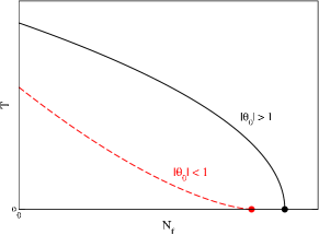
Figure 1: The generic thermal transition lines for the power law $|N^{c}_{f,0}-N_{f}|^{-\frac{1}{\Theta_{0}}}$ with cases $|\Theta_{0}|<1$ and $|\Theta_{0}|>1$. The quantum critical points for zero temperature are marked with filled circles.

In principle there are two possible generic scenarios for the power law with $|\Theta_{0}|>1$ and $|\Theta_{0}|<1$, shown in Fig. 1. For $|\Theta_{0}|>1$, the phase transition line approaches the zero temperature axis with infinite slope, whereas for $|\Theta_{0}|<1$ the slope vanishes at the quantum critical point. In QCD, predictions for $\Theta_{0}$ from the functional renormalization group approach arXiv:0912.4168 ; Braun:2010qs are consistent with recent results from lattice simulations arXiv:1110.3152 and result in $|\Theta_{0}|<1$.

In this work we investigate the corresponding behavior of QED₃ under the presence of anisotropies with $v_{F}=v_{\Delta}\neq c_{s}$. As a tool to determine the relevant critical temperatures, we use the Dyson–Schwinger equations (DSEs) for the (anisotropic) fermion propagator of the theory. Due to the anisotropic setup, the three momentum directions have to be treated separately, which prevents the introduction of hyperspherical coordinates in the Dyson–Schwinger equations. It turned out that a natural framework to deal with this situation is the formulation of the DSEs in a finite volume, i.e. in a box with antiperiodic boundary conditions. This approach, originally introduced in Refs. Fischer:2002eq ; Fischer:2005nf , has been used to study the finite volume behavior of isotropic QED₃ as well as the behavior of $N_{f}^{c}$ at zero temperature in the anisotropic setup Bonnet:2011hh . The results agreed qualitatively with corresponding ones in other frameworks Thomas:2006bj ; Concha:2009zj , thus underlining the feasibility of the approach. In this work we generalize the approach to include finite temperature effects. As it turns out, we obtain values of $|\Theta_{0}|$ that depend on the size of anisotropy.

This work is organized as follows: In the next section we discuss the structure of the Dyson–Schwinger equations (DSEs) of anisotropic QED₃ at finite temperature as well as the truncation scheme we are using. We also summarize some issues concerning the formulation of the DSEs in a box. In section III we present our results and discuss the scaling properties around the quantum critical point and comment on finite volume effects. We finish with a short summary and conclusions.

II Technical details

II.1 The Dyson–Schwinger equations in anisotropic $\mbox{QED}_{3}$ at finite temperatures

The details of the formulation of anisotropic QED₃ have been discussed in Refs. Franz:2002qy ; Lee:2002qza ; Hands:2004ex and summarized in Ref. Bonnet:2011hh . Here we only state the most essential details, using the notation of Ref. Franz:2002qy . The fermionic four component spinors obey the Clifford algebra $\{\gamma_{\mu},\gamma_{\nu}\}=2\,\delta_{\mu\nu}$. We consider $N_{f}\,$ fermion flavors and the anisotropic fermionic velocities $v_{F}\,$ and $v_{\Delta}\,$ which will be implemented via a factor $g_{i,\mu\nu}$ acting like a metric. The index i = 1,2 indicates the node in consideration. In the high-temperature superconducting (HTS) system, the different nodes correspond to different zeroes of the fermionic energy gap function placed on the Fermi surface of the HTS system Herbut:2002yq .

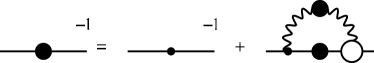
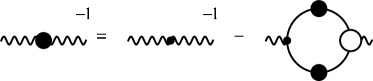
Figure 2: The diagrammatic representation of the Dyson–Schwinger equations for the fermion (a) and gauge boson propagator (b). Wiggly lines denote photon propagators, straight lines fermion propagators. A blob denotes a dressed propagator or vertex, whereas a dot stands for a bare fermion-photon vertex.

The metric for the first node is given by

$$\left(g_{i=1}^{\mu\nu}\right)=\left(\begin{array}[]{ccc}1&0&0\\ 0&\,v_{F}\,^{2}&0\\ 0&0&v_{\Delta}\,^{2}\end{array}\right),$$ (2)

whereas the metric for the second node can be obtained from interchanging the fermionic velocities. It enters the Lagrangian in the form of

$$\mathcal{L}^{aniso}=\frac{N_{f}}{2}\sum_{j=1,2}\bar{\Psi}_{j}\left\{\sum_{\mu=0}^{2}\gamma_{\nu}\sqrt{g}_{j,\nu\mu}\left(i\partial_{\mu}-a_{\mu}\right)\right\}\Psi_{j}.$$ (3)

The order parameter for chiral symmetry breaking is the chiral condensate which can be determined via the trace of the dressed fermion propagator

$$S_{F,j}(\omega_{p},\vec{p})=\int^{\beta}_{0}d\tau\int\frac{d^{2}x}{(2\pi)^{2}}e^{i\omega_{p}\tau-i\vec{p}\vec{x}}\langle\bar{\Psi}_{j}(\tau,\vec{x})\Psi_{j}(0,0)\rangle,$$ (4)

with inverse temperature $\beta=1/T$ and spacial momentum $\vec{p}=(p_{1},p_{2})^{T}$. The corresponding expression for the dressed photon propagator is given by

$$D_{\mu\nu}(\omega_{p},\vec{p})=\int_{0}^{\beta}d\tau\int\frac{d^{2}x}{(2\pi)^{2}}e^{i\omega_{p}\tau-i\vec{p}\vec{x}}\langle A_{\mu}(\tau,\vec{x})A_{\nu}(0,0)\rangle,$$ (5)

and the Matsubara frequencies in both equations read

$$\omega_{p}=2\pi T\left\{\begin{array}[]{cc}n_{t}+\frac{1}{2}&\mbox{for fermions}\\ n_{t}&\mbox{for bosons }\end{array}\right.$$ (6)

with integer numbers $n_{t}$.

Diagrammatically, the Dyson–Schwinger equations are represented in Fig. 2 and Fig. 2. In Euclidean space-time at non-zero temperatures, they are explicitly given by

$$S_{F,j}^{-1}(\omega_{p},\vec{p})\; = S_{0,j}^{-1}(\,\omega_{p},\vec{p}\,)\;\;+\,Z_{1}\,e^{2}\,T\sum_{n_{t}}\int\frac{d^{2}q}{(2\pi)^{2}}(\sqrt{g}_{j,\mu\alpha}\gamma^{\alpha}S_{F,j}(\,\omega_{q},\vec{q}\,)\sqrt{g}_{j,\nu\beta}\Gamma^{\beta}(\,\omega_{q},\vec{q},\omega_{p},\vec{p}\,)\,D_{\mu\nu}(\,\omega_{k},\vec{k}\,)),$$ (7)

$$D_{\mu\nu}^{-1}(\omega_{p},\vec{p}) = D_{0,\mu\nu}^{-1}(\omega_{p},\vec{p}\,)-\frac{Z_{1}e^{2}TN_{f}}{2}\sum_{\tiny\begin{array}[]{c}j=1,2;\\ n_{t}\end{array}}\int\frac{d^{2}q}{(2\pi)^{2}}\mbox{Tr}\left[\sqrt{g}_{j,\mu\alpha}\gamma^{\alpha}S_{F,j}(\omega_{q},\vec{q}\,)\sqrt{g}_{j,\nu\beta}\Gamma^{\beta}(\omega_{p},\vec{p},\omega_{q},\vec{q}\,)S_{F,j}(\omega_{k}\vec{k}\,)\right],$$ (10)

with the momentum $\,k_{\mu}\,$ defined by the difference $p_{\mu}-q_{\mu}$ and the node index $i=1,2$. The inverse bare fermion propagator is given by $S_{0,j}^{-1}(p)=Z_{2}i\gamma_{\nu}\,\sqrt{g}_{j,\nu\mu}\,p_{\mu}$ with $p=(\,\omega_{p},\vec{p})$ and the inverse bare photon propagator is given by $D_{0,\mu\nu}^{-1}(p)=Z_{3}p^{2}P^{T}_{\mu\nu}(p)$ with transverse projector $P^{T}$. The dressed fermion-boson vertex is denoted by $\Gamma^{\beta}(\,p_{\mu},q_{\mu}\;)$. The renormalization constants $Z_{1}$, $Z_{2}$ and $Z_{3}$ of vertex, fermion and gauge boson respectively are each defined by the ratio of renormalized to unrenormalized dressing function of the corresponding one-particle irreducible Greens’ function. Since QED₃ is ultraviolet finite, all renormalization constants can be set to one without loss of generality. The Ward-identity $Z_{1}=Z_{2}$ is then trivially satisfied.

Since we consider anisotropic space-time, we have to take care of the individual dressing of the Dirac components of the fermions at the different nodes. In order to keep track of the general structure of the equations we use the shorthands Bonnet:2011hh :

$$\overline{p}_{i}^{2}:=p_{\mu}\;g_{i}^{\mu\nu}\;p_{\nu}$$ (11)

and

$$\widetilde{p}_{\mu,i}:=A_{\mu,i}\left(\omega_{p},\vec{p}\;\right)p_{\mu},\mbox{ (no summation convention !), }$$ (12)

where $A_{\mu,i}$ denotes the vectorial fermionic dressing function at node $i$.

The anisotropic expressions for the dressed fermion and photon propagators then read

$$S_{F,i}^{-1}\left(\omega_{p},\vec{p}\;\right) = B_{i}\left(\omega_{p},\vec{p}\;\right)+\mbox{i}\;\sqrt{g_{i}}^{\mu\nu}\gamma_{\nu}\;\widetilde{p}_{\mu,i},$$ (13)

$$D_{\mu\nu}\left(\omega_{p},\vec{p}\;\right)^{{}^{-1}} = p^{2}\left(\delta_{\mu\nu}-\frac{p_{\mu}p_{\nu}}{p^{2}}\right)+\Pi_{\mu\nu}\left(\omega_{p},\vec{p}\;\right),\,\,\,\,\,$$ (14)

where $B_{i}$ denotes the scalar fermion dressing function at node i and $\Pi_{\mu\nu}\left(\,\omega_{p},\vec{p}\;\right)$ the vacuum polarization of the gauge boson field.

Next we explain our approximation scheme for the DSEs of the fermion and photon propagator. One of the most employed schemes is the $1/N_{f}$ expansion, which led to some success in the early analysis of the chiral transition at large $N_{f}$ and zero temperature Appelquist:1988sr ; Nash:1989xx . In this approximation the vector part of the fermion propagator is just a constant, i.e. dressing effects in the fermion wave function are not taken into account. Later on it turned out that this approximation is too drastic and leads to the wrong behavior of the photon propagator in the chirally symmetric phase. In Ref. Fischer:2004nq it was shown that a self-consistent calculation of the coupled system of fermion and photon-DSEs beyond the $1/N_{f}$ approximation leads to nontrivial power laws of the photon and fermion wave functions in the symmetric phase with values of irrational exponents depending on the details of the approximation for the fermion-photon vertex. A nontrivial fermion wave function beyond $1/N_{f}$ was also shown to be important to correctly determine the dependencies of the chiral transition on $N_{f}$ in the presence of non-zero anisotropies Bonnet:2011hh . We therefore have to take into account these effects here as well. To this end we employ the same approximation scheme as detailed in Ref. Bonnet:2011hh . We use a form for the fermion-photon vertex that agrees with its Ward-Takahashi identity to leading order in the tensor structures. This ansatz is given by

$$\Gamma^{\beta}_{i}(\omega_{p},\vec{p},\omega_{q},\vec{q})=\gamma^{\beta}\frac{A^{\beta}_{i}(\omega_{p},\vec{p})+A^{\beta}_{i}(\omega_{q},\vec{q})}{2}$$ (15)

without using summation convention and the fermionic momenta $p,q$ at the vertex. In the gauge sector we are currently not able to solve the photon DSE self-consistently for general anisotropies. We therefore approximate the photon self-energy by a model which is closely built along the self-consistent result of the isotropic case. In particular it takes into account the irrational power laws discovered in Ref. Fischer:2004nq . The gauge boson vacuum polarization then reads

$$\Pi^{\mu\nu}\left(p\;\right) = \sum_{i}\sqrt{\overline{p}_{i}^{2}}\left(g_{i}^{\mu\nu}-\frac{g_{i}^{\mu\alpha}p_{\alpha}\;g_{i}^{\nu\delta}p_{\delta}}{\overline{p}_{i}^{2}}\right)\,\,\Pi_{i}\left(p\right)\,,$$

$$\Pi_{i}\left(p\right) = \frac{e^{2}N_{f}}{16\,v_{F}v_{\Delta}}\left(\frac{1}{\sqrt{\overline{p}_{i}^{2}}}\frac{\overline{p}_{i}^{2}}{\overline{p}_{i}^{2}+e^{2}}+\frac{1}{\overline{p}_{i}^{1+2\kappa}}\frac{e^{2}}{{\overline{p}_{i}}^{2}+e^{2}}\right)\,,$$

with $\overline{p}_{i}^{2}$ defined in Eq. (11) and $p=(\,\omega_{p},\vec{p})$. In Ref. Fischer:2004nq the value of $\kappa$ for the vertex truncation Eq. (LABEL:model) at the critical number of fermion flavors $N_{f}^{c}$ has been determined as $\kappa=0.0358$. In principle, this number may depend on the fermion velocities in the anisotropic case. Nevertheless, due to our current inability to calculate this dependence we will keep $\kappa$ constant in all calculations. We also fix the gauge coupling $e^{2}=1$ independent of the value of $N_{f}$ and temperature $T$. This choice is one of many possible ones that serve to compare theories with different numbers of fermion flavors $N_{f}$.

Having specified our approximations (15),(LABEL:model), we now proceed with the fermion-DSE. In order to extract the scalar and vector dressing function of the fermion we take appropriate traces of the fermion-DSE and rearrange the equations to end up with

$$B_{i}\left(\omega_{p},\vec{p}\;\right) = \;Te^{2}\sum_{n_{t}}\int\frac{d^{2}q}{\left(2\pi\right)^{2}}\frac{B_{i}\left(\omega_{q},\vec{q}\;\right)g_{i}^{\mu\nu}D_{\mu\nu}(\omega_{k},\vec{k}\;)}{B_{i}\left(\omega_{q},\vec{q}\;\right)^{2}+(\overline{\widetilde{q}}_{i,\mu}\;)^{2}},$$ (17)

$$A_{\mu,i}\left(\omega_{p},\vec{p}\;\right) = 1-\frac{Te^{2}}{p_{\mu}}\sum_{n_{t}}\int\frac{d^{2}q}{\left(2\pi\right)^{2}}\left\{\frac{2\left(\widetilde{q}_{\lambda,i}\;g_{i}^{\lambda\nu}D_{\mu\nu}(\omega_{k},\vec{k}\;)\right)-\widetilde{q}_{\mu,i}\;g_{i}^{\lambda\nu}D_{\lambda\nu}(\omega_{k},\vec{k}\;)}{B_{i}\left(\omega_{q},\vec{q}\;\right)^{2}+(\;\overline{\widetilde{q}}_{i,\mu}\;)^{2}}\right\}\frac{A_{\mu,i}(\omega_{p},\vec{p})+A_{\mu,i}(\omega_{q},\vec{q})}{2},$$ (18)

where again we have no summation for the external index $\mu$. In the following, we will investigate the finite temperature equations in case of equal fermionic velocities $v_{F}\,=v_{\Delta}\,$, reducing the fermionic vector dressing function to two instead of three different components and leaving us with only one sort of nodes. We therefore drop the nodal index $i$.

II.2 The DSEs on a torus

Considering anisotropy and additional finite temperatures, the computational demands increase significantly in comparison to the isotropic vanishing temperature investigations, even despite the applied approximations for the gauge boson. We therefore continue our investigations by changing the basic manifold from three-dimensional Euclidean spacetime to a three-torus, which is well suited for the evaluation of the Cartesian sums emerging from the boundary conditions the fermion and boson fields have to obey. To be precise, only the time direction for the boson has to be periodic and for the fermion field antiperiodic. The spacelike components are chosen to show the same (anti-)periodicity as the time component of the according field for convenience. In order to guarantee a valid interpretation of the timelike direction as a temperature, we have to make sure that the aspect ratio of time- and spacelike ’boxlength’ is appropriate. We therefore distinguish the boxlength in coordinate space as $L_{1}\sim 1/T$ in time direction and equal lengths $L_{2}=L_{3}=L_{X}$ in spacelike directions. The momentum integrals are then also replaced by Matsubara sums,

$$\int\frac{d^{2}q\,}{(2\pi)^{2}}\>(\cdots)\>\>\longrightarrow\>\>\frac{1}{L_{X}^{2}}\sum_{n_{2},n_{3}}\>(\cdots)\,.$$ (19)

The discrete fermionic momenta are then counted by ${\bf q}_{\bf n}=\sum_{i=2,3}(2\pi/L_{X})(n_{i}+1/2)\hat{e}_{i}$, where $\hat{e}_{i}$ represents a Cartesian unit vector in Euclidean momentum space. For the photon with periodic boundary conditions the momentum counting goes like ${\bf q}_{\bf n}=\sum_{i=2,3}(2\pi/L_{X})(n_{i})\hat{e}_{i}$. The resulting system of equations can be solved numerically along the lines described in Ref. Goecke:2008zh .

As already discussed in the course of previous investigations Bonnet:2011hh ; Goecke:2008zh , evaluations on a finite volume have a considerable impact on the quantitative results for the critical number of fermion flavors, but hardly change the qualitative behavior, when considering anisotropies. Since the introduction of finite temperature is conceptually very similar to the previously studied anisotropies, we expect similar findings for volume extrapolations and postpone detailed studies on this subject. Instead, we concentrate again on the variations of $N_{f}^{c}$, keeping in mind that its absolute number will change in infinite volume calculations.

III Numerical results

III.1 The critical $\mbox{N}_{f}^{c}$ in the anisotropic case $v_{F}\,=v_{\Delta}\,$

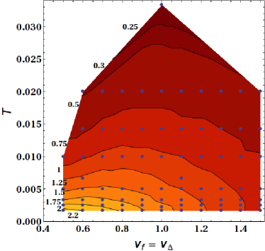
Figure 3: The critical number of fermion flavors, $N_{f}^{c}$ plotted as a function of the fermionic velocities $v_{F}\,=v_{\Delta}\,$, and the temperature $T$.

In this section we present our results on the finite temperature phase diagram for the case of equal anisotropic velocities $v_{F}\,=v_{\Delta}\,$ with $c_{s}=1$. We obtain the phase diagram for the critical number of fermion flavors, $N_{f}^{c}$, from solving the set of Dyson–Schwinger equations (17) and (18) on a torus of $(N_{X}^{2}=39^{2})\times(N_{T}=23)$ points and a box length of $e^{2}L_{X}=600$. In time direction, the sum of $N_{T}=23$ Matsubara frequencies guarantee a reasonable aspect ratio between the spacial and temporal number of lattice points, necessary for finite temperature calculations. The order parameter for chiral symmetry breaking is the chiral condensate ($tr_{D}$ denotes the trace in Dirac-space),

$$\langle\bar{\Psi}\Psi\rangle=T\sum_{n_{t}}\int\frac{d^{2}q}{(2\pi)^{2}}tr_{D}S_{F}(\omega_{q},\vec{q})$$ (20)

or, equivalently, the value of the scalar fermion dressing function $B(\omega_{q},\vec{q})$ at the lowest Matsubara frequency and two-momentum. For each given temperature and anisotropy we determined the critical number of fermion flavors $N_{f}^{c}$.

The results of our calculations are shown in Fig. 3. The critical number of fermion flavors has been determined numerically at each dot in the diagram. Subsequently a Mathematica interpolation routine converted these values into areas of equal $N_{f}^{c}$ in different colors separated by contour lines. The contour lines therefore have to be taken as approximate results from the interpolation procedure and only serve to guide the eye. In agreement with our previous investigations Bonnet:2011hh we find a decreasing critical number of fermion flavors for increasing anisotropy at effective zero temperature. When we increase the temperature at fixed anisotropy we again find a decreasing $N_{f}^{c}$ for all anisotropic velocities taken into account. It is noteworthy that for anisotropic velocities larger than the isotropic value, $v_{F}\,=v_{\Delta}\,\geq 1$, this decrease happens at a comparably slow rate, while for $v_{F}\,=v_{\Delta}\,\leq 1$ the critical number of fermion flavors rapidly falls off with increasing temperatures.

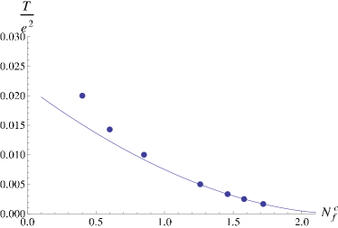
Figure 4: The critical temperature for the chiral transition as a function of the number of fermion flavors for the case $v_{F}\,=v_{\Delta}\,=0.8$. Shown are our numerical results together with a fit of the power law (22) in the region $N_{f}>1.25$, i.e. in the vicinity of the quantum transition.

III.2 Scaling in the pseudo-conformal phase transition region

There is a considerable number of works identifying the chiral phase transition in QED₃ as of pseudo-conformal nature due to the dimensionful coupling constant $\alpha$, see e.g. Miransky:1988gk ; Gusynin:1998kz ; Fischer:2004nq and references therein. The scaling behavior close to the phase transition relates QED₃ with other strongly coupled theories such as many-flavor QCD that has been subject to a number of recent studies in the framework of renormalization group equations Gies:2005as ; Braun:2005uj ; Braun:2006jd ; arXiv:0912.4168 ; Kaplan:2009kr ; Braun:2010qs ; Braun:2011pp . These investigations have shown that the explicit form of the symmetry-breaking scale, $k_{SB}$, is to zeroth order given by the expression

$$k_{SB} \sim k_{0}\theta(N^{c}_{f,0}-N_{f})|N^{c}_{f,0}-N_{f}|^{-\frac{1}{\Theta_{0}}}$$ (21)

$$\times\mbox{exp}\left(-\frac{a}{\sqrt{|N^{c}_{f,0}-N_{f}|}}\right),$$

where $k_{0}$ denotes a scale-fixing constant and $N^{c}_{f,0}$ is the critical fermion number for chiral symmetry breaking at zero temperature. Furthermore, $\Theta_{0}$ represents the leading order term in the Taylor expansion of the critical exponent $\Theta$ in $|N_{f,0}^{c}-N_{f}|$ and $a$ a further parameter. Whereas the form of the scaling relation (21) has been derived from very general considerations and is therefore universal for strongly flavored asymptotically free gauge theories, the parameter $a$ depends on the theory in question, see Ref. Braun:2010qs for details. A similar type of scaling law also applies to observables such as the critical temperature.

In a formulation of the theory on a finite volume it is extremely difficult to assess the complete scaling law (21). Exponential Miransky scaling dominates (21) only very close to the critical fermion number and therefore cannot be resolved within the temperature range available in such a setup. This is also the case for our formulation of the DSEs on a torus. In the following we therefore strive to identify the power law part of the scaling relation, which is expected to dominate further away from $N_{f,0}^{c}$ until finally a value of $|N_{f,0}^{c}-N_{f}|$ is reached where scaling ceases altogether. In the following we seek to locate the region where the power law scaling

$$T_{cr}\sim k_{0}|N^{c}_{f,0}-N_{f}|^{-\frac{1}{\Theta_{0}}}$$ (22)

is applicable. We come back to this point below.

As an example consider the case of $v_{F}\,=v_{\Delta}\,=0.8$ shown in Fig. 4. The power law (22) nicely fits the calculated points in the region $1.25<N_{f}<1.75$. For $N_{f}<0.9$ significant deviations of the calculated critical temperatures from the scaling law occur indicating the finite extent of the scaling region. For $N_{f}>1.75$, somewhere close to $N^{c}_{f,0}$ we expect the exponential Miransky scaling finally to dominate over (22). This region can only be investigated in the (even more demanding) continuum formulation of the DSEs, which we will address in future work.

The values for $|\Theta_{0}|$ and the corresponding critical fermion numbers $N_{f,0}^{c}$ at zero temperature are given in Figs. 6 and 6. In general we observed that the size of the scaling region where the power law (22) can be found, depends on the value of $|\Theta_{0}|$. It is quite large for $|\Theta_{0}|<1$, as can be seen in Fig. 4, but turned out to be much smaller for $|\Theta_{0}|>1$ and consequently the extracted values for $\Theta_{0}$ in this case have to be treated with some caution.

Fig. 6 shows that the anisotropic velocities provide a parameter that qualitatively changes the scaling behavior close to the quantum critical point $N_{f,0}^{c}$. Shown are results for our standard torus of $(N_{X}^{2}=39^{2})\times(N_{T}=23)$ points and a spatial box length of $e^{2}L_{X}=600$, denoted by red dots. In order to assess the effects of finite volume we also determined three selected points (the crosses) on an even larger torus with $(N_{X}^{2}=59^{2})\times(N_{T}=23)$ and $e^{2}L_{X}=900$, requiring a considerable increase in invested computational resources. Finite volume effects are clearly present and tend to amplify the results for the critical exponent. However, this quantitative impact is rather uniform with respect to changes in the anisotropy, a finding in agreement with similar estimates in the zero temperature caseBonnet:2011hh . We therefore conclude that our results serve very well to identify at least the qualitative behavior of $|\Theta_{0}|(v_{f})$. We find a maximum with a critical exponent much larger than one in the isotropic case $v_{F}\,=v_{\Delta}\,=1$. For smaller anisotropies, $0.5<v_{F}\,=v_{\Delta}\,<0.9$, the critical exponent decreases rapidly to values smaller than one, $|\Theta_{0}|<1$, while for larger anisotropies $1.1<v_{F}\,=v_{\Delta}\,<1.5$ the decrease is slower.

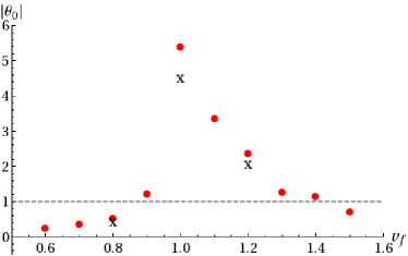
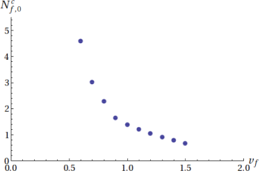
Figure 5: The critical exponent $|\Theta_{0}|$ plotted as a function of the fermionic velocities $v_{F}\,=v_{\Delta}\,$. Red dots indicate results obtained with a box length of $L_{X}=600/e^{2}$, whereas the crosses indicate results on the larger torus with $L_{X}=900/e^{2}$

Figure 6: The critical number of fermion flavors for zero temperature, $N^{c}_{f,0}$ plotted as a function of the fermionic velocities $v_{F}\,=v_{\Delta}\,$.

The size of the exponent $\Theta_{0}$ is a measure for the size of the power law corrections to exponential Miransky scaling close to $N_{f,0}^{c}$, as discussed in Ref. Braun:2010qs . These corrections are induced by the running of the gauge coupling determined by the photon polarization Eq. (LABEL:model) and found to be small for $|\Theta_{0}|\gg 1$ and large for $|\Theta_{0}|\ll 1$. Thus the large value of $|\Theta_{0}|\approx 5$ for the isotropic case indicates the presence of dominant exponential Miransky-scaling with only very small power law corrections. On the other hand, for anisotropies $v_{F}\,=v_{\Delta}\,<0.9$ the power law corrections dominate. Unfortunately at present we cannot further quantify this issue since the exponential Miransky scaling region very close to $N_{f,0}^{c}$ is typically small (see Table 2 in Ref. Braun:2011pp for an estimate) and therefore not accessible in our formulation on a torus, as discussed above. Nevertheless we may be able to qualitatively infer the size of the scaling region by going further away from $N_{f,0}^{c}$. Indeed, as discussed above, we find a larger scaling region there for $|\Theta_{0}|<1$, whereas for $|\Theta_{0}|>1$ the scaling region is much smaller in agreement with the considerations above and in Ref. Braun:2010qs .

The zero-temperature critical number of fermion flavors (Fig. 6) decreases for increasing anisotropies thus confirming the behavior already found in Ref. Bonnet:2011hh . Note that the zero-temperature fit of the critical number of fermion flavors is not identical to our previous results. The (small) deviations arise from the fact, that both calculations were performed on similar, but not equally sized tori.

IV Summary and conclusions

In this work we have determined the critical temperature for the chiral phase transition of anisotropic QED₃ as a function of the number of fermion flavors $N_{f}$ for different anisotropies. To this end we solved a coupled set of truncated DSEs for the anisotropic fermion propagator together with model input for the photon self energy determined from the isotropic case at $T=0$. We found a generic phase diagram with decreasing critical temperature with increasing $N_{f}$. The transition line hits the $N_{f}$-axis at the quantum critical point $N_{f,0}^{c}$. We investigated the critical scaling with $N_{f}$ around the critical point and verified a universal scaling law determined on general grounds for strongly coupled asymptotically free gauge theories in Refs. arXiv:0912.4168 ; Braun:2010qs . A characteristic quantity that characterizes this scaling region is the critical exponent $|\Theta_{0}|$. We found that the anisotropic velocities provide a parameter that drives QED₃ from a setting with $|\Theta_{0}|$ smaller than one to a region with large values of the critical exponent $|\Theta_{0}|\gg 1$. This result is interesting but preliminary, since the gauge sector of the theory was not taken into account dynamically in our framework. Thus the full consequences of our findings can only be addressed when fully self-consistent solutions of the fermion- and photon-DSEs are available. Nevertheless, our present framework serves as a qualitative guide and constitutes a proof of principle for the feasibility of dealing with anisotropic systems in strongly interacting fermionic theories.

References

- (1) F. Sannino, Acta Phys. Polon. B 40 (2009) 3533 [arXiv:0911.0931 [hep-ph]].
- (2) A. Cheng, A. Hasenfratz and D. Schaich, arXiv:1111.2317 [hep-lat].
- (3) K. Ogawa, T. Aoyama, H. Ikeda, E. Itou, M. Kurachi, C. J. D. Lin, H. Matsufuru and H. Ohki et al., arXiv:1111.1575 [hep-lat].
- (4) M. Franz, Z. Tesanovic and O. Vafek, Phys. Rev. B 66 (2002) 054535 [arXiv:cond-mat/0203333]; Z. Tesanovic, O. Vafek, and M. Franz, Phys. Rev. B 65 (2002) 180511 [arXiv:cond-mat/0110253]; M. Franz and Z. Tesanovic, Phys. Rev. Lett. 87, (2001) 257003. [arXiv:cond-mat/0012445];
- (5) I. F. Herbut, Phys. Rev. B 66, 094504 (2002) [arXiv:cond-mat/0202491]; Phys. Rev. Lett. 88 (2002) 047006 [arXiv:cond-mat/0110188].
- (6) K. S. Novoselov et al., Nature 438 (2005) 197 [arXiv:cond-mat/0509330].
- (7) M. Chiao, et al. Phys. Rev. B 62 (2000) 3554
- (8) D. J. Lee and I. F. Herbut, Phys. Rev. B 66, 094512 (2002) [arXiv:cond-mat/0201088].
- (9) S. Hands and I. O. Thomas, Phys. Rev. B 72, 054526 (2005) [arXiv:hep-lat/0412009].
- (10) I. O. Thomas and S. Hands, Phys. Rev. B 75, 134516 (2007) [arXiv:hep-lat/0609062]; PoS LAT2005, 249 (2006) [arXiv:hep-lat/0509038].
- (11) A. Concha, V. Stanev and Z. Tesanovic, Phys. Rev. B 79 (2009) 214525 [arXiv:0906.1103 [cond-mat.supr-con]].
- (12) J. A. Bonnet, C. S. Fischer, R. Williams, Phys. Rev. B 84 (2011) 024520 [arXiv:1103.1578 [hep-ph]]; arXiv:1111.0182 [hep-ph].
- (13) J. Braun and H. Gies, JHEP 1005 (2010) 060 [arXiv:0912.4168 [hep-ph]].
- (14) J. Braun, C. S. Fischer, H. Gies, Phys. Rev. D 84 (2011) 034045 [arXiv:1012.4279 [hep-ph]].
- (15) J. Braun, J. Phys. G G 39 (2012) 033001 [arXiv:1108.4449 [hep-ph]].
- (16) K. Miura, M. P. Lombardo and E. Pallante, arXiv:1110.3152 [hep-lat].
- (17) C. S. Fischer, R. Alkofer and H. Reinhardt, Phys. Rev. D 65 (2002) 094008 [arXiv:hep-ph/0202195]; C. S. Fischer, B. Gruter and R. Alkofer, Annals Phys. 321 (2006) 1918 [arXiv:hep-ph/0506053]; C. S. Fischer, A. Maas, J. M. Pawlowski and L. von Smekal, Annals Phys. 322, 2916 (2007) [arXiv:hep-ph/0701050].
- (18) C. S. Fischer and M. R. Pennington, Phys. Rev. D 73 (2006) 034029 [arXiv:hep-ph/0512233]; Eur. Phys. J. A 31 (2007) 746 [arXiv:hep-ph/0701123]; J. Luecker, C. S. Fischer and R. Williams, Phys. Rev. D 81 (2010) 094005 [arXiv:0912.3686 [hep-ph]].
- (19) T. Appelquist, D. Nash and L. C. R. Wijewardhana, Phys. Rev. Lett. 60 (1988) 2575.
- (20) D. Nash, Phys. Rev. Lett. 62 (1989) 3024.
- (21) C. S. Fischer, R. Alkofer, T. Dahm and P. Maris, Phys. Rev. D 70 (2004) 073007 [arXiv:hep-ph/0407104].
- (22) T. Goecke, C. S. Fischer and R. Williams, Phys. Rev. B 79 (2009) 064513 [arXiv:0811.1887 [hep-ph]].
- (23) V. P. Gusynin, V. A. Miransky and A. V. Shpagin, Phys. Rev. D 58 (1998) 085023 [arXiv:hep-th/9802136].
- (24) V. A. Miransky, K. Yamawaki, Mod. Phys. Lett. A4 (1989) 129-135; Phys. Rev. D55 (1997) 5051-5066. [hep-th/9611142].
- (25) H. Gies and J. Jaeckel, Eur. Phys. J. C 46, 433 (2006) [arXiv:hep-ph/0507171].
- (26) J. Braun and H. Gies, Phys. Lett. B 645, 53 (2007) [arXiv:hep-ph/0512085].
- (27) J. Braun and H. Gies, JHEP 0606, 024 (2006) [arXiv:hep-ph/0602226].
- (28) D. B. Kaplan, J. W. Lee, D. T. Son and M. A. Stephanov, Phys. Rev. D 80, 125005 (2009) [arXiv:0905.4752 [hep-th]].
- (29) J. Braun, Phys. Rev. D 81 (2010) 016008 [arXiv:0908.1543 [hep-ph]].