Cosmic string evolution with a conserved charge

Abstract

Cosmic strings with degrees of freedom beyond the standard Abrikosov-Nielsen-Olesen or Nambu-Goto strings are ubiquitous in field theory as well as in models with extra dimensions, such as string theoretic brane inflation scenarios. Here we carry out an analytic study of a simplified version of one such cosmic string model. Specifically, we extend the velocity-dependent one-scale (VOS) string evolution model to the case where there is a conserved microscopic charge on the string worldsheet. We find that whether the standard scale-invariant evolution of the network is preserved or destroyed due to the presence of the charge will crucially depend on the amount of damping and energy losses experienced by the network. This suggests, among other things, that results derived in Minkowski space (field theory) simulations may not extend to the case of an expanding universe.

I Motivation

Cosmic strings Vilenkin and Shellard (1994); Hindmarsh and Kibble (1995), line-like topological defects that can be produced in cosmological phase transitions, provide a valuable tool for constraining models of the early universe. Having a wide range of potential observational signals Copeland et al. (2011), which depend directly on their microphysical properties, they can be used to constrain high-energy physics parameters from cosmological observations. In particular, the magnitude of their observational signatures is mainly determined by the energy scale of the corresponding symmetry breaking transition. Interest in the study of cosmic strings has been renewed in recent years Kibble (2004) with the realisation that string-like defects are generic in a wide range of fundamental models, including Supersymmetric Grand Unified Theories Jeannerot et al. (2003) and Brane Inflation models in String Theory Burgess et al. (2001); Sarangi and Tye (2002); Dvali and Vilenkin (2004); Copeland et al. (2004). In the latter case, there is even the exciting possibility of constraining (within a given model) fundamental parameters like the string coupling, string scale, and warping/compactification scales from cosmological observations Pourtsidou et al. (2011); Avgoustidis et al. (2011); Copeland et al. (2011).

In order to be able to make this quantitative link between late time observations and early universe physics, one must therefore be able to model the evolution of string networks from the time of their formation until they are observed. Work in this direction has mostly focused on the simplest, structureless strings of the Abrikosov-Nielsen-Olesen type and their corresponding Nambu-Goto thin string approximations. In recent years, more complex models have been developed (both on the numerical Copeland and Saffin (2005); Urrestilla and Vilenkin (2008); Hindmarsh and Saffin (2006); Sakellariadou and Stoica (2008) and analytical Tye et al. (2005); Avgoustidis and Shellard (2008); Avgoustidis and Copeland (2010) fronts), allowing for the formation of zipping interactions between strings of different tensions, in order to describe the richer nature of the so called FD-networks Polchinski (2004) that appear in Brane Inflation models.

However, even networks of a single type of string can have non-trivial internal structure, generally carrying additional degrees of freedom on the string worldsheet. This is the generic situation in models with extra dimensions, where there is a proliferation of scalar fields that can couple to (and condense on) the strings. Cosmic strings with additional worldsheet degrees of freedom (scalar charges, currents, fermionic zero-modes) have been extensively studied in field theory and supergravity, see for example Witten (1985); Callan and Harvey (1985); Davis and Shellard (1988); Ganoulis and Lazarides (1989); Carter and Peter (1995); Brax et al. (2006). One important result that emerged from these studies was the realisation that the presence of currents can lead to the formation of stable cosmic string loops, known as vortons Davis and Shellard (1988, 1989), which could therefore dominate the energy density of the universe. This has allowed to obtain strong bounds on models producing vortons Brandenberger et al. (1996); Martins and Shellard (1998a, b).

To date, the cosmological evolution of such string networks remains largely unexplored. It is therefore desirable to understand how these additional degrees of freedom can be described macroscopically, and how their presence affects the behaviour and cosmological consequences of the corresponding string networks. In a recent paper Nunes et al. (2011), the evolution of semilocal strings Vachaspati and Achucarro (1991) was described analytically and it was found that the spectrum of scaling solutions has a much richer structure than in ordinary cosmic strings. The presence of worldsheet degrees of freedom would also modify significantly the structure of scaling network solutions and can be expected to obstruct scaling, possibly leading to string frustration.

Here, we focus on the case of cosmic strings with a conserved charge living on the string worldsheet. We extend the VOS model Martins and Shellard (1996a, b, 2002); Martins et al. (2004) to describe this case analytically, and study the effect of the charge on the evolution of the string network. A recent related example, for the case of domain walls, comes from the work of Battye et al. Battye et al. (2009) (but see also Battye and Pearson (2010) for some caveats), who suggest that with a conserved, homogeneous and localised Noether charge the number of domain walls does not scale in the usual way, in which case they could provide some contribution to the dark energy suggested by cosmological observations. These results are based on relatively small numerical simulations in $2+1$ dimensions and without cosmological expansion, so extrapolating them to a cosmological context requires some care. Nevertheless, they highlight the need for a better macroscopic description of these processes. As we shall see, our analysis will provide some possible explanations for these results.

II Microscopic model

Here we review the basics of the microscopic model that we will be using. This model is described in detail in Ref. Martins and Shellard (1998a). A comprehensive description of the general formalism can be found in Carter (1997).

II.1 Generic chiral models

For strings carrying conserved currents, we consider the Witten-Carter-Peter (chiral) model, which implicitly makes use of the fact that in two dimensions a conserved current can be written as the derivative of a scalar field. The dynamics is described by the Witten action

$$S_{W}=\int\sqrt{-\gamma}\left[-\mu_{0}+\frac{1}{2}\gamma^{ab}\phi_{,a}\phi_{,b}-qA_{\mu}x^{\mu}_{,a}\frac{\tilde{\epsilon}^{ab}}{\sqrt{-\gamma}}\phi_{,b}\right]d^{2}\sigma-\frac{1}{16\pi}\int d^{4}x\sqrt{-g}F_{\mu\nu}F^{\mu\nu}\,,$$ (1)

where the four terms are respectively the usual Nambu-Goto term ($\mu_{0}$ being the string tension and $\gamma$ the pullback of the background metric $g$ on the worldsheet), the inertia of the charge carriers described by the scalar $\phi$, the current coupling to the electromagnetic potential $A_{\mu}$, and the kinetic term for the electromagnetic field. Worldsheet indices are denoted by $a,b\in\{0,1\}$ and we will take $\sigma^{0}$ to be the timelike coordinate, while $\sigma^{1}\equiv\sigma$ will be spacelike; $\tilde{\epsilon}^{ab}$ is the alternating tensor in two dimensions. Note that this action applies to both the bosonic and the fermionic case.

We are essentially interested in the chiral limit of this model, that is (taking dot/prime to denote differentiation with respect to the timelike/spacelike worldsheet coordinate $\sigma^{0}$/$\sigma$):

$$\phi^{\prime}{}^{2}=\epsilon^{2}{\dot{\phi}}^{2}\,,$$ (2)

where $\epsilon$ is the scalar

$$\epsilon\equiv\frac{-{x^{\prime}}^{2}}{\sqrt{-\gamma}}\,,$$ (3)

giving the string energy per unit coordinate length. Let us now consider an FRW background

$$ds^{2}=a^{2}(d\tau^{2}-d{\bf x}^{2})$$ (4)

and choose the standard gauge

$$\sigma^{0}=\tau\,,\qquad{\dot{\bf x}}\cdot{\bf x}^{\prime}=0\,,$$ (5)

in which the scalar $\epsilon$ becomes:

$$\epsilon={\left(\frac{{\bf x}^{\prime}{}^{2}}{1-{\dot{\bf x}}^{2}}\right)}^{1/2}\,.$$ (6)

Then, in the chiral limit, introducing the simplifying function $\Phi$ defined as

$$\Phi(\phi)=\frac{{\dot{\phi}}^{2}}{\mu_{0}a^{2}(1-{\bf{\dot{x}}}^{2})}\,,$$ (7)

the microscopic equations of motion take the form Martins and Shellard (1998a):

$$\left[\epsilon\left(1+\Phi\right)\right]{\dot{}}+\frac{\epsilon}{\ell_{d}}{\dot{\bf x}}^{2}=\Phi^{\prime}-2\frac{{\dot{a}}}{a}\epsilon\Phi\,,$$ (8)

and

$$\epsilon\left(1+\Phi\right){\ddot{\bf x}}+\frac{\epsilon}{\ell_{d}}(1-{\dot{\bf x}}^{2}){\dot{\bf x}}=\left[\left(1-\Phi\right)\frac{{\bf x}^{\prime}}{\epsilon}\right]^{\prime}+\left({\dot{\Phi}}+2\frac{{\dot{a}}}{a}\Phi\right){\bf x}^{\prime}+2\Phi{\dot{\bf x}}^{\prime}\,,$$ (9)

where for simplicity we have introduced the damping length

$$\frac{1}{\ell_{d}}=a\left(2H+\frac{1}{\ell_{\rm f}}\right)\,,$$ (10)

describing Hubble friction ($H=a^{-1}(da/dt)={\dot{a}}/a^{2}$), but also allowing for an additional friction mechanism with characteristic lengthscale $\ell_{\rm f}$.

Two generic useful relations are

$$\frac{\dot{\epsilon}}{\epsilon}=\frac{{\dot{\bf x}}\cdot{\ddot{\bf x}}}{1-{\dot{\bf x}}^{2}}-\frac{{\dot{\bf x}}\cdot{\bf x}^{\prime\prime}}{{\bf x^{\prime}}{}^{2}}$$ (11)

and

$$\frac{\epsilon^{\prime}}{\epsilon}=\frac{{\bf x}^{\prime}\cdot{\bf x}^{\prime\prime}}{{\bf x^{\prime}}{}^{2}}-\frac{{\bf x}^{\prime}\cdot{\ddot{\bf x}}}{1-{\dot{\bf x}}^{2}}\,.$$ (12)

The curvature vector $d^{2}{\bf x}/ds^{2}$, with $ds=\sqrt{{\bf x}^{\prime}{}^{2}}d\sigma$, satisfies:

$$\frac{d^{2}{\bf x}}{ds^{2}}=\frac{{\bf x}^{\prime\prime}}{{\bf x^{\prime}}{}^{2}}-\frac{({\bf x^{\prime}}\cdot{\bf x}^{\prime\prime}){\bf x^{\prime}}}{{\bf x^{\prime}}{}^{4}}\,.$$ (13)

Thus, a curvature radius, $R$, can be defined locally via

$$\frac{\dot{\bf x}}{\epsilon(1-{\dot{\bf x}}^{2})}\cdot\left(\frac{{\bf x^{\prime}}}{\epsilon}\right)^{\prime}=-\frac{{\bf x^{\prime}}\cdot{\dot{\bf x^{\prime}}}}{{\bf x^{\prime}}{}^{2}}=\frac{{\bf x}^{\prime\prime}\cdot{\dot{\bf x}}}{{\bf x^{\prime}}{}^{2}}=\frac{a}{R}({\dot{\bf x}}\cdot{\bf u})\,,$$ (14)

where we have introduced a unit vector $\bf u$ in the direction of the curvature vector.

The worldsheet charge and current densities are respectively given by

$$\rho_{w}=q\epsilon{\dot{\phi}}\,,$$ (15)

and

$$j_{w}=q\frac{\phi^{\prime}}{\epsilon}\,,$$ (16)

while the total energy of a piece of string is given by

$$E=\mu_{0}a\int\left(1+\Phi\right)\epsilon d\sigma=E_{s}+E_{\Phi}\,.$$ (17)

We can immediately interpret the energy (17) as being split in an obvious way into a string component and a charge component. Defining a macroscopic charge as the average of $\Phi$ over the string worldsheet, we then have:

$$Q=\langle\Phi\rangle\equiv\frac{\int\Phi\epsilon d\sigma}{\int\epsilon d\sigma}=\frac{E_{\Phi}}{E_{s}}\,.$$ (18)

This interpretation will be relevant below.

Introducing the network string density $\rho_{s}$ such that $E_{s}\propto\rho_{s}a^{3}$ and defining the correlation length $\xi$ by

$$\rho_{s}=\frac{\mu_{0}}{\xi^{2}}\,,$$ (19)

the evolution equations have the form

$$\frac{\dot{E}_{s}}{E_{s}}=\frac{\dot{\rho}_{s}}{\rho_{s}}+3\frac{\dot{a}}{a}=-2\frac{\dot{\xi}}{\xi}+3\frac{\dot{a}}{a}=\frac{\dot{a}}{a}+\left\langle\frac{\dot{\epsilon}}{\epsilon}\right\rangle\,,$$ (20)

$$v^{2}=\langle{\dot{\bf x}}^{2}\rangle\,,\quad v{\dot{v}}=\langle{\dot{\bf x}}\cdot{\ddot{\bf x}}\rangle$$ (21)

and

$${\dot{Q}}=\langle{\dot{\Phi}}\rangle\,.$$ (22)

Two further (not independent) useful relations are

$$\frac{\dot{E}_{\Phi}}{E_{\Phi}}=\frac{\dot{Q}}{Q}+\frac{\dot{E}_{s}}{E_{s}}\,,$$ (23)

and

$$\frac{\dot{E}}{E}=\frac{\dot{E}_{s}}{E_{s}}+\frac{\dot{Q}}{1+Q}=\frac{\dot{\rho}}{\rho}+3\frac{\dot{a}}{a}=-2\frac{\dot{L}}{L}+3\frac{\dot{a}}{a}\,,$$ (24)

where $\rho\propto Ea^{-3}$ is the energy density and the lengthscale $L$ is defined by:

$$\rho=\frac{\mu_{0}}{L^{2}}\,.$$ (25)

With these, one can in principle proceed to average this model. An additional difficulty which is absent in the case of Nambu-Goto strings is the appearance of a term proportional to (${\bf x}^{\prime}\cdot{\bf x}^{\prime\prime}$). This factor is not expected to be zero even though (${\bf x}^{\prime}\cdot{\bf u}$) is, see equation (13). This will be discussed in more detail below.

Finally, note that in the case of the VOS model for plain Nambu-Goto strings one assumes that the network has a single characteristic length scale, so that $R=L=\xi$. This is no longer true in the charged case, but we will still assume that $R=\xi$, while $L$ is now only a measure of the total energy in the network.

II.2 Conserved microscopic charge case

In our particular case we have

$$\rho_{w}=q\epsilon{\dot{\phi}}=q\phi^{\prime}=const.$$ (26)

and therefore

$$\Phi=\frac{\varphi_{0}^{2}}{a^{2}{\bf x^{\prime}}{}^{2}}\,,$$ (27)

with $\varphi_{0}$ being a constant. Now, by simple differentiation one finds that $\Phi$ evolves as follows

$${\dot{\Phi}}+2\frac{\dot{a}}{a}\Phi=2\Phi\frac{{\dot{\bf x}}\cdot{\bf x}^{\prime\prime}}{{\bf x^{\prime}}{}^{2}}$$ (28)

and

$$\Phi^{\prime}+2\Phi\frac{{\bf x}^{\prime}\cdot{\bf x}^{\prime\prime}}{{\bf x^{\prime}}{}^{2}}=0\,.$$ (29)

The conserved charge assumption simplifies some of the above equations. If one expands Eq. (11) by successively substituting in Eqs. (8-9) and then Eqs. (28-29) one obtains

$${\ddot{\bf x}}\cdot{\bf x}^{\prime}=\frac{{\bf x}^{\prime}\cdot{\bf x}^{\prime\prime}}{\epsilon^{2}}\,,$$ (30)

and inserting this in Eq. (12) yields

$$\epsilon^{\prime}=0\,.$$ (31)

An alternative way to see this is to substitute Eq. (9) into Eq. (12) and then use Eqs. (28-29). This leads to

$$\frac{2\Phi}{1+\Phi}\frac{\epsilon^{\prime}}{\epsilon}=0\,,$$ (32)

thus if $\Phi\neq 0$ we must have $\epsilon^{\prime}=0$.

III Interlude: Nambu-Goto Strings in Extra Dimensions

The above formalism describing strings with currents is also analogous to the effective description of structureless, Nambu-Goto strings evolving in the presence of compact extra dimensions. Indeed, integrating out the extra dimensions gives rise to worldsheet scalars which geometrically correspond to string positions in the internal manifold and behave like currents in the low energy worldsheet theory.

The evolution and dynamics of strings moving in spacetimes with extra compact dimensions have been studied in Ref. Avgoustidis and Shellard (2005). Consider the following ‘augmented’ FRW metric

$$ds^{2}=dt^{2}-a(t)^{2}d{\bf x}^{2}-b(t)^{2}d{\bf l}^{2}\,,$$ (33)

where the internal manifold (coordinates $\bf l$) has been taken for simplicity to be toroidal with scalefactor $b(t)$. Now let the vector $\bf l(\tau,\sigma)$ denote the string position in this internal manifold. In the simplest static case, $b(t)=1$, the string energy is:

$$\varepsilon_{e} \equiv \frac{-x^{\prime}{}^{2}}{\sqrt{-\gamma}}={\left(\frac{{\bf x}^{\prime}{}^{2}+{\bf l}^{\prime}{}^{2}/a^{2}}{1-{\dot{\bf x}}^{2}-{\dot{\bf l}}^{2}/a^{2}}\right)}^{1/2}$$

$$\simeq {\left(\frac{{\bf x}^{\prime}{}^{2}}{1-{\dot{\bf x}}^{2}}\right)}^{1/2}\left(1+1/2\frac{{\bf l}^{\prime}{}^{2}}{a^{2}{\bf x}^{\prime}{}^{2}}+1/2\frac{{\dot{\bf l}}^{2}}{a^{2}(1-{\dot{\bf x}}^{2})}\right)\,,$$

where we have expanded to linear order in ${\bf l}^{\prime}{}^{2}/(a^{2}{\bf x}^{\prime}{}^{2})$ and ${\dot{\bf l}}^{2}/[a^{2}(1-{\dot{\bf x}}^{2})]$.

The analogy to the above discussion is apparent: the first factor in the last line of (III) is simply $\epsilon$, while the terms in the second factor are of the form of equations (7) and (2). Indeed, setting ${\dot{\bf l}}^{2}/[a^{2}(1-{\dot{\bf x}}^{2})]=\Phi$, and considering the analogue of the ‘chiral limit’ $\phi^{\prime}{}^{2}=\epsilon^{2}\dot{\phi}^{2}$ discussed above, we then have in this case

$${\bf l}^{\prime}{}^{2}=\frac{{\bf x}^{\prime}{}^{2}}{(1-{\dot{\bf x}}^{2})}{\dot{\bf l}}^{2}\,,$$ (35)

and equation (III) becomes

$$\varepsilon_{e}\simeq\epsilon(1+\Phi)$$

in direct analogy to equation (17). In addition, the equation of motion for $\varepsilon_{e}$

$$\frac{\dot{\varepsilon}_{e}}{\varepsilon_{e}}=-\frac{\dot{a}}{a}\left[1+{\dot{\bf x}}^{2}-{\bf x}^{\prime}{}^{2}/\varepsilon_{e}^{2}\right]$$ (36)

with $\varepsilon_{e}\simeq\epsilon(1+\Phi)$ becomes:

$$\left[\epsilon\left(1+\Phi\right)\right]{\dot{}}=-2\frac{{\dot{a}}}{a}\epsilon({\dot{\bf x}}^{2}+\Phi)+\mathcal{O}(\Phi^{2})\,,$$ (37)

which is equation (8) for $\Phi^{\prime}=0$ to linear order in $\Phi$.

Note that this analogy only becomes quantitative in the limit where ${\bf l}^{\prime}{}^{2}/(a^{2}{\bf x}^{\prime}{}^{2})$ and ${\dot{\bf l}}^{2}/[a^{2}(1-{\dot{\bf x}}^{2})]$ are small. The embedding fields ${\bf l}\equiv l^{m}$ ($m=1,...,D$), describing the string positions in the $D$ compact extra dimensions, are worldsheet scalars which in general have richer dynamics than in action (1). In particular, their kinetic structure is governed by the relativistic action Nambu-Goto action in $4+D$ spacetime dimensions:

$$S=-\mu_{0}\int\sqrt{-{\rm det}\left(g^{(4)}_{\mu\nu}\partial_{a}x^{\mu}\partial_{b}x^{\nu}+g^{(D)}_{\ell m}\partial_{a}l^{\ell}\partial_{b}l^{m}\right)}\,,$$ (38)

where $g^{(4)}_{\mu\nu}$ is the (4-dimensional) spacetime metric and $g^{(D)}_{\ell m}$ the metric in the $D$ compact dimensions. Factoring out $\gamma^{(4)}_{ab}\equiv g^{(4)}_{\mu\nu}\partial_{a}x^{\mu}\partial_{b}x^{\mu}$ yields:

$$S=-\mu_{0}\int\sqrt{-{\rm det}\gamma^{(4)}_{ab}}\sqrt{{\rm det}(\delta^{a}_{b}+\gamma_{(4)}^{ac}\,\partial_{c}l^{\ell}\partial_{b}l^{m}\,g^{(6)}_{\ell m})}\,,$$ (39)

that is, the general action for the worldsheet scalars has non-trivial kinetic structure. However, for small $\dot{l}$ and $l^{\prime}$, the second factor in (39) can be linearised, and with the additional ‘chiral’ condition (35) one recovers the first two terms of the Witten action (1), for $D$ scalars, $l^{m}$, subject to (35).

IV Loop solutions

Simple exact loop solutions can be used to further our understanding of the role of the various terms on the evolution of the strings, and also determine the accuracy of averaged (macroscopic) quantities in relation to microscopic quantities. The simplest loop solution is a circular one, which has the form

$$\ {\bf x}={r(\tau)(\cos{\theta},\sin{\theta},0)}$$ (40)

with

$$\epsilon=\frac{r}{\sqrt{1-\dot{r}^{2}}}\,,\quad\Phi=\frac{\varphi_{0}^{2}}{a^{2}r^{2}}\,,$$ (41)

and

$$E=\mu_{0}a\int\left(1+\frac{\varphi^{2}}{a^{2}r^{2}}\right)\epsilon d\sigma\,.$$ (42)

For this ansatz Eqs. (8) and (9) are equivalent, and either of them can then be written

$$(1+\Phi)\ddot{r}+(1-\dot{r}^{2})\left[2\frac{\dot{a}}{a}{\dot{r}}+(1-\Phi)\frac{1}{r}\right]=0\,,$$ (43)

while the evolution equation for $\Phi$ has the form

$$\dot{\Phi}=-2\Phi\left(H+\frac{\dot{r}}{r}\right)\,,$$ (44)

which is in fact trivial given the definition of $\Phi$ in (41).

We start by examining the case with no expansion ($H=0$). The evolution equations, Eqs. (8) and (9), now simplify to

$$\epsilon(1+\Phi)=const.=1\,$$ (45)

and

$$\ddot{r}+(1-\Phi^{2})r=0\,.$$ (46)

Alternatively, they can be written as

$$\dot{r}^{2}+r^{2}=1-2\varphi_{0}^{2}-4\frac{\varphi_{0}^{4}}{r^{2}}\,$$ (47)

and

$$\ddot{r}+r=\frac{\varphi_{0}^{4}}{r^{3}}\,.$$ (48)

These have periodic (oscillatory) solutions, but unlike the case of circular loops in the plain Nambu-Goto case, the presence of a charge ensures that these loops never collapse to zero size and that their microscopic velocity is always less than unity. Indeed, the maximum velocity is

$$\dot{r}^{2}_{\rm max}=1-4\varphi_{0}^{2}\,.$$ (49)

The limiting behaviour corresponds to a static solution,

$$r=\varphi_{0}=\frac{1}{2}\,,\quad\dot{r}=0\,;$$ (50)

in this solution the energy of the loop is equally divided, half of it being in the string itself and the other half in the current. In the general case, the average loop velocity (over one oscillation period) is

$$\langle\dot{r}^{2}\rangle=\frac{1}{2}(1-4\varphi_{0}^{2})\,,$$ (51)

and the average fraction of the loop’s total energy in the current is

$$\left\langle\frac{E_{\Phi}}{E}\right\rangle=\varphi_{0}\,;$$ (52)

naturally the rest of the energy corresponds to the (bare) string. Finally the macroscopic charge of these loops, given by Eq. (18), is

$$Q=\frac{\varphi_{0}}{1-\varphi_{0}}\,;$$ (53)

notice that this is unity in the static limit ($\varphi_{0}=1/2$). The static solution we discussed above still exists in an expanding universe. In this case it corresponds to

$$ar=\varphi_{0}\,,\quad\dot{r}=0;$$ (54)

such a loop will have a physical radius

$$R_{\rm phys}=\frac{ar}{\sqrt{1-\dot{r}^{2}}}=\varphi_{0}\,.$$ (55)

Solving the differential equation for r and integrating over one period, we can obtain

$$\frac{\langle\dot{\bf{x}}^{2}\rangle^{2}}{\langle\dot{\bf{x}}^{4}\rangle}=\frac{2}{3}$$ (56)

which is the same as in the case without charge. This result is important because the fact that it is always of order unity allows us to, every time a microscopic quantity such as $\dot{\bf x}^{4}$ appears in an expression inside an integral, average it to $v^{4}$ to a good approximation. In the general case with expansion, Eq. (43) cannot be solved analytically, but numerically we found that this result still holds to a good approximation for a wide range of initial conditions. Fig. 1 shows the behaviour of a particular solution, for which we find

$$\frac{\langle\dot{\bf{x}}^{2}\rangle^{2}}{\langle\dot{\bf{x}}^{4}\rangle}\sim 0.6622\,.$$ (57)

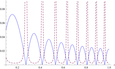
Figure 1: The time evolution of a particular loop solution in an expanding universe. The solid (blue) curve shows $r$, while the dashed (red) one shows the force $\varphi_{0}^{4}/r^{3}$ due to the charge, Eq. (48). As the loop shrinks and $r$ approaches zero, the force provides a ‘boost’ causing it to expand again.

As can be seen in Fig. 1, the charge in the loops keeps them from reaching $r=0$ by providing a ‘boost’ when $r$ is approaching zero. It then causes $r$ to grow again (to a lower value than before), while it returns to its previous value. Naturally, these simple loop solutions satisfy Eqs. (30-31), and indeed one can check that this is still the case for Kibble-Turok Kibble and Turok (1982) and Burden Burden (1985) loops.

V Macroscopic equations

We can now proceed and look at the averaged evolution equations in our conserved microscopic charge case.

V.1 General dynamical equations

The total energy of the string is given by Eq. (17) and therefore we can define two characteristic lengths for the string, as in section II.1; the usual correlation length $\xi$ associated with the string energy

$$E_{s}=\mu a\int{\epsilon d\sigma}\propto\rho_{s}a^{3}\,,$$ (58)

through Eqn. (19), and the lengthscale $L$ associated with the total energy $E\propto\rho a^{3}$, see Eqs. (17), (25). Taking the time derivative of the previous equation, one easily finds the evolution equation for $\xi$

$$2\frac{\dot{\xi}}{\xi}=2H\left(1+\frac{v^{2}}{1+Q}\right)+\frac{2Q}{1+Q}\frac{kv}{R}-\left\langle\frac{\Phi^{\prime}}{\epsilon(1+\Phi)}\right\rangle\,.$$ (59)

Here, $k$ is the so-called ‘momentum parameter’ quantifying the average angle between the curvature vector and the velocity of string segments in the network. It thus provides a measure of the small-scale-structure on strings and can range from 0 (wiggly strings in flat space) to order unity (smooth strings) Martins and Shellard (2002).

Correspondingly, the evolution equation for L is

$$2\frac{\dot{L}}{L}=2H\left(1+\frac{v^{2}+Q}{1+Q}\right)-\left\langle\frac{\Phi^{\prime}}{\epsilon(1+\Phi)}\right\rangle\,.$$ (60)

As was defined above, Eqn. (18), the macroscopic charge $Q$ is the averaged microscopic charge $\langle\Phi\rangle$, which is also the ratio between the string energy $E_{s}$ and the ‘charge’ energy $E_{\Phi}$. Differentiating (18), we find that its evolution equation is

$$\frac{\dot{Q}}{Q}=2\left(\frac{kv}{R}-H\right)$$ (61)

Finally, the string velocity is defined by

$$v^{2}=\langle{\dot{\bf{x}}^{2}}\rangle=\frac{\int\dot{\bf{x}}^{2}\epsilon d\sigma}{\int\epsilon d\sigma}\,,$$ (62)

and taking time derivatives on both sides, we arrive at the evolution equation

$$\dot{v}=\frac{1-v^{2}}{1+Q}\left[\frac{k}{R}(1-Q)-2Hv+\frac{1+Q}{v}\left\langle\frac{\Phi^{\prime}}{\epsilon(1+\Phi)}\right\rangle\right]$$ (63)

However, equations (59), (60) and (61) are not independent: there is a consistency relation between $\xi$ and $L$

$$E_{s}=\frac{E}{1+Q}\longrightarrow\xi=L\sqrt{1+Q}$$ (64)

Therefore, the equations are related by

$$2\frac{\dot{L}}{L}=2\frac{\dot{\xi}}{\xi}-\frac{\dot{Q}}{1+Q}\,,$$ (65)

which is verified, so the three equations are consistent.

V.2 Ansatz for the charge gradient

As previously mentioned, in order to proceed we now need to deal with the (${\bf x}^{\prime}\cdot{\bf x}^{\prime\prime}$) term coming from $\Phi^{\prime}$. Referring to Eq. (29), dimensional analysis suggests an ansatz of the form

$$\left\langle\frac{\Phi^{\prime}}{\epsilon(1+\Phi)}\right\rangle=-s\frac{v}{R}\frac{2Q}{1+Q}$$ (66)

where $s$ is (at least, to a first approximation) a constant.

Using (66) and noting our earlier identification $R=\xi$, our evolution equations become:

$$2\frac{\dot{\xi}}{\xi}=2H\left(1+\frac{v^{2}}{1+Q}\right)+\frac{2Q}{1+Q}\frac{(k+s)v}{\xi}\,$$ (67)

$$2\frac{\dot{L}}{L}=2H\left(1+\frac{v^{2}+Q}{1+Q}\right)+\frac{2Q}{(1+Q)^{3/2}}\frac{sv}{L}\,$$ (68)

$$\frac{\dot{Q}}{Q}=2\left(\frac{kv}{\xi}-H\right)\,$$ (69)

$$\dot{v}=\frac{1-v^{2}}{1+Q}\left[\frac{k}{\xi}\left(1-Q(1+2s/k)\right)-2Hv\right]\,.$$ (70)

We will assume a critical-density universe with generic expansion rates of the form

$$a\propto t^{\lambda}\,,\quad H=\frac{\lambda}{t}\,,$$ (71)

and look for scaling solutions of the form

$$\xi=\xi_{0}t^{\alpha}$$ (72)

(or an analogous law for $L$),

$$v=v_{0}t^{\beta}\,,$$ (73)

and

$$Q=Q_{0}t^{\gamma}\,.$$ (74)

Note that causality implies $\alpha\leq 1$ and the finite speed of light implies $\beta\leq 0$. Furthermore, our discussion of loop solutions shows that $v\to 1$ is not a physically allowed solution for these networks.

VI No charge losses

In this section we assume that there are no macroscopic charge losses. (The case with charge losses will be discussed in the following section.) We will separately consider the cases with and without energy losses due to loop production.

Whether or not we have loop production, the evolution equation for the macroscopic charge $Q$ is given by Eq. (69), and we can start by studying this. There is a trivial but unphysical (refer to discussion after Eqn. (59)) solution if $k=0$, with $\xi\propto L\propto a$ and $v\propto Q\propto a^{-2}$, which can therefore be ignored. In the realistic case $k\neq 0$ there can in principle be two kinds of solutions:

• Decaying charge solutions, with

  $$\gamma=-2\lambda\,,\quad\beta<\alpha-1\,;$$ (75)

  for these solutions not only does the charge decay (as $Q\propto a^{-2}$) but velocity will necessarily decay as well.

• standard solutions with

  $$\beta=\alpha-1\,,\quad\gamma=-2\lambda+2k\frac{v_{0}}{\xi_{0}}\,;$$ (76)

  here we have used the term ‘standard’ referring to the fact that linear scaling solution (with $\alpha=1$ and $\beta=0$) is of this form, although a priori there is no guarantee that this solution will exist with a constant (non-zero) charge. Also note that in this branch of solutions we may at least in principle have growing, constant, or decaying $Q$.

We can now study the entire system of equations in the cases with and without energy losses.

VI.1 Without energy losses

In this case we obtain the following three scaling relations:

• For slow expansion rates, $\lambda<2/3$,

  $$\alpha=\frac{3}{2}\lambda<1\,,\quad\xi_{0}=\frac{kv_{0}}{\lambda}$$ (77)

  $$\beta=\alpha-1<0$$ (78)

  $$\gamma=0\,,\quad Q_{0}=\left(1+\frac{2s}{k}\right)^{-1}\,$$ (79)

  and

  $$\frac{\rho_{s}}{\rho_{crit}}\propto\frac{\rho}{\rho_{crit}}\propto t^{2-3\lambda}\,;$$ (80)

  here we have a constant charge, which gradually slows the strings (making $v\to 0$), although the evolution is still faster than conformal stretching (which corresponds to $\alpha=\lambda$). As a consequence, both the energy density in the strings and the total energy density in the network grow relative to that of the cosmological background.

• For $\lambda=2/3$, corresponding to the matter-dominated era,

  $$\alpha=1\,,\quad\xi_{0}=\frac{3}{2}kv_{0}$$ (81)

  $$\beta=0\,,\quad v_{0}^{2}=\frac{1}{2}\left[1-Q_{0}\left(1+\frac{2s}{k}\right)\right]$$ (82)

  $$\gamma=0$$ (83)

  and

  $$\frac{\rho_{s}}{\rho_{crit}}=\frac{1}{1+Q_{0}}\frac{\rho}{\rho_{crit}}=\frac{16\pi}{3k^{2}}\left[1-Q_{0}\left(1+\frac{2s}{k}\right)\right]^{-1}G\mu\,;$$ (84)

  in this case the macroscopic charge is still a constant, but the additional dilution caused by the faster expansion rate is enough to ensure that the energy density of the network is a constant fraction of the background one. In other words, for this particular expansion rate we have a generalised linear scaling solution, with $\xi$ (and $L$) growing as fast as allowed by causality, in which the RMS velocity and the macroscopic charge are constant (and larger charges leading to smaller velocities, as was seen in the loop solutions).

• For fast expansion rates, $\lambda>2/3$,

  $$\alpha=1\,,\quad\xi_{0}^{2}=\frac{k^{2}}{4\lambda(1-\lambda)}$$ (85)

  $$\beta=0\,,\quad v_{0}^{2}=\frac{1-\lambda}{\lambda}$$ (86)

  $$\gamma=4-6\lambda<0$$ (87)

  and

  $$\frac{\rho_{s}}{\rho_{crit}}=\frac{\rho}{\rho_{crit}}=\frac{32\pi}{3k^{2}}\frac{1-\lambda}{\lambda}G\mu\,;$$ (88)

  here the additional Hubble damping makes the macroscopic charge decay, and we therefore end up with the solution for ordinary Nambu-Goto strings Kibble (1985); Martins and Shellard (1996a, b).

Therefore, which of these solutions is the attractor for the network’s evolution depends on the universe’s expansion rate, which is parametrized by $\lambda$. (In principle, one also finds a fourth solution which has $v_{0}=1$, but, according to our discussion in the loops section, this is unphysical for charged strings.) By numerically solving the evolution equations one can confirm that the above solutions are indeed the attractors in the relevant parameter ranges; Fig. 2 shows examples for the two scaling regimes.

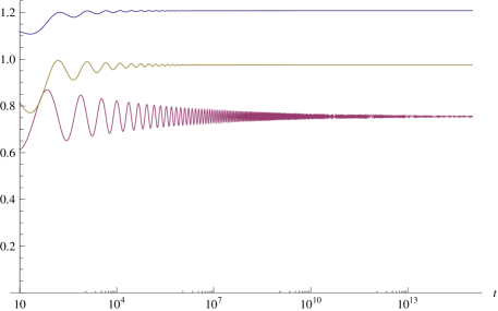
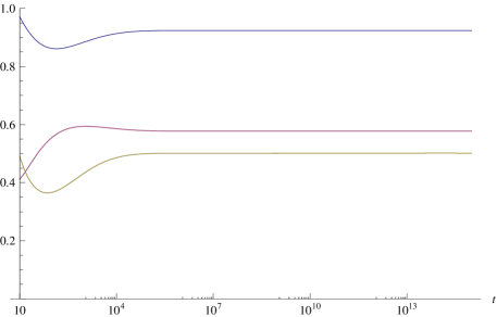
Figure 2: Illustrating the two scaling solutions in the case without energy losses. The plots show the relevant macroscopic quantities divided by the time dependencies inferred in this section’s analysis, so that asymptotically constant values imply convergence to the expected scaling solution. Top panel: Case $\lambda=1/2$; from top to bottom the lines depict $\xi/t^{3/4}$, $Q$ and $vt^{1/4}$. Bottom panel: Case $\lambda=3/4$; from top to bottom the lines depict $\xi/t$, $v$ and $Qt^{1/2}$. In both cases we have assumed $k=0.8$ and $s=0.01$.

VI.2 With energy losses

The loss of energy through loop production is described by a new term in the evolution equation for $\dot{\xi}$ (and, consequently, one for $\dot{L}$), which, using standard arguments Kibble (1985); Martins and Shellard (1996a, b), one can write as

$$2\frac{\dot{\xi}}{\xi}=...+\frac{cv}{\xi}\,.$$ (89)

This introduces the parameter $c$ quantifying the efficiency of producing loops. Similarly, using Eq. (65) and assuming there is no charge loss, we find the equivalent term for $\dot{L}$,

$$2\frac{\dot{L}}{L}=...+\frac{cv}{L}\frac{1}{\sqrt{1+Q}}\,.$$ (90)

The analysis of scaling solutions can now be repeated, and one finds solutions that generalise the above ones by including an additional dependency on the loop chopping efficiency $c$:

• For slow expansion rates, $\lambda<2/(3+c/k)$,

  $$\alpha=\frac{1}{2}\left(3+\frac{c}{k}\right)\lambda<1\,,\quad\xi_{0}=\frac{kv_{0}}{\lambda}$$ (91)

  $$\beta=\alpha-1<0$$ (92)

  $$\gamma=0\,,\quad Q_{0}=\left(1+\frac{2s}{k}\right)^{-1}\,$$ (93)

  and

  $$\frac{\rho_{s}}{\rho_{crit}}\propto\frac{\rho}{\rho_{crit}}\propto t^{2-(3+c/k)\lambda}\,;$$ (94)

  loop production is an additional energy loss mechanism, and therefore the correlation length now grows faster than in the $c=0$ case. Similarly, string velocities decrease more slowly, and the network’s density grows more slowly relative to the background one.

• For an intermediate expansion rate, $\lambda=2/(3+c/k)$,

  $$\alpha=1\,,\quad\xi_{0}=\frac{1}{2}v_{0}\left(3k+c\right)$$ (95)

  $$\beta=0\,,\quad v_{0}^{2}=\frac{1}{2}\left[1-Q_{0}\left(1+\frac{2s}{k}\right)\right]$$ (96)

  $$\gamma=0$$ (97)

  and

  $$\frac{\rho_{s}}{\rho_{crit}}=\frac{1}{1+Q_{0}}\frac{\rho}{\rho_{crit}}=\frac{16\pi}{3k^{2}}\left[1-Q_{0}\left(1+\frac{2s}{k}\right)\right]^{-1}G\mu\,;$$ (98)

  now the expansion rate for which this solution occurs decreases, with the smaller expansion rate being compensated, for the purposes of the dilution of the network’s energy density, by the process of loop production. (For $c=0$ this solution exists for the matter era, and $c=k$ will make it occur in the radiation era.) Interestingly, the ratio of the string and background energies is exactly the same as before—in other words, it does not depend on the value of $c$.

• For fast expansion rates, $\lambda>2/(3+c/k)$,

  $$\alpha=1\,,\quad\xi_{0}^{2}=\frac{k(k+c)}{4\lambda(1-\lambda)}$$ (99)

  $$\beta=0\,,\quad v_{0}^{2}=\frac{1-\lambda}{\lambda}\frac{k}{k+c}$$ (100)

  $$\gamma=\frac{4}{k+c}\left[k-\frac{\lambda}{2}(3k+c)\right]<0$$ (101)

  and

  $$\frac{\rho_{s}}{\rho_{crit}}=\frac{\rho}{\rho_{crit}}=\frac{32\pi}{3k(k+c)}\frac{1-\lambda}{\lambda}G\mu\,;$$ (102)

  this is exactly the VOS linear scaling solution for Nambu-Goto strings Martins and Shellard (1996a, b, 2002); Martins et al. (2004), with an added prediction of a particular decay law for the charge (which depends on the cosmological expansion rate).

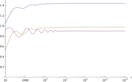
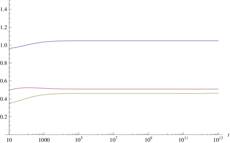
Figure 3: Illustrating the two scaling solutions in the case with energy losses. The plots show the relevant macroscopic quantities divided by the time dependencies inferred in this section’s analysis, so that asymptotically constant values imply convergence to the expected scaling solution. Top panel: Case $\lambda=1/2$; from top to bottom the lines depict $\xi/t^{0.822...}$, $Q$ and $vt^{0.178...}$. Bottom panel: Case $\lambda=3/4$; from top to bottom the lines depict $\xi/t$, $v$ and $Qt^{0.723...}$. In both cases we have assumed $k=0.8$, $c=0.23$ and $s=0.01$.

Fig. 3 illustrates the two branches of the solution. It can be trivially seen that in the limit of no loop production, $c\to 0$, these solutions are the same as in the case without energy losses, Eqns. (77)-(88). As before, there is a fourth solution with $v=1$ which is not allowed for charged strings. The analysis so far also highlights the point that the parameter $c$ is important for determining whether charge survives on the strings or decays. This motivates a discussion of possible charge losses, which will be done in the next section.

VII Macroscopic charge losses

In the previous section, in order to derive the energy loss term in the evolution equation for $L$, it was assumed that there was no charge loss. Now this assumption will be dropped, and the resulting scaling relations analysed. This section is somewhat more phenomenological than the rest of the article, since it will rely on simplifying assumptions for how the charge may be lost, but our goal is simply to develop an intuitive picture for the possible role of charge loss mechanisms on the evolution of the network.

We will again assume an energy loss term of the form

$$\frac{\dot{E}_{s}}{E_{s}}=-c\frac{v}{\xi}\,,\quad 2\frac{\dot{\xi}}{\xi}=...+c\frac{v}{\xi}$$ (103)

but this time let us say that $L$ gets a different (in general) loss term

$$\frac{\dot{E}}{E}=-fc\frac{v}{L}\,,\quad 2\frac{\dot{L}}{L}=...+fc\frac{v}{L}\,,$$ (104)

where $f$ is an arbitrary function, possibly of the velocity, charge and correlation length. We are therefore assuming that any such charge losses are related to the network’s intercommuting and loop production mechanisms.

In the previous section, we assumed there was no charge loss, implicitly using

$$f(v,Q,\xi)=\frac{1}{\sqrt{1+Q}}\,.$$ (105)

Instead, we will now leave $f$ free and obtain the evolution equation for $Q$ from the above assumptions together with Eq. (65). The result is

$$\dot{Q}=2Q(\frac{kv}{\xi}-H)+\frac{cv}{\xi}(1+Q)\left(1-f\sqrt{1+Q}\right)\,,$$ (106)

or an analogous equation in terms of $L$. With the choice (105) for $f$ we trivially recover the results of the previous sections. We can now look for scaling relations as before, checking how the results depend on the choice of $f$.

We start by noting that, in the standard VOS-model case (without a charge), we would not expect charge to be created. Therefore, $\dot{Q}=0$ when $Q=0$, implying

$$2\frac{cv}{\xi}(1-f)=0\,.$$ (107)

It then follows that, if the function $f$ is constant, it has to be equal to unity. Otherwise it must be dependent on the charge (and possibly other quantities), and become unity when the charge drops to zero,

$$f=f(Q,v,\xi)\implies f(0,v,\xi)=1\,,$$ (108)

as was the case for the function (105) we used in the case without charge loss.

Let us therefore consider the $f=1$ case. The generalised scaling laws now become:

• For slow expansion rates, $\lambda<(2k-Wc)/[3k+(1-W)c]$,

  $$\alpha=\frac{3}{2}\left[\frac{1+(1-W)c/3k}{1-Wc/2k}\right]\lambda<1\,,\quad\xi_{0}=\frac{v_{0}}{\lambda}(k-Wc/2)$$ (109)

  $$\beta=\alpha-1<0$$ (110)

  $$\gamma=0\,,\quad Q_{0}=\left(1+\frac{2s}{k}\right)^{-1}\,$$ (111)

  and naturally

  $$\frac{\rho_{s}}{\rho_{crit}}\propto\frac{\rho}{\rho_{crit}}\propto t^{2(1-\alpha)}\,$$ (112)

  (where for simplicity we have kept $\alpha$ in the last expression); we have also introduced

  $$W=(1+Q_{0}^{-1})\left(\sqrt{1+Q_{0}}-1\right)\,,$$ (113)

  which is always positive and behaves as $W=0.5(1+Q_{0})$ in the limit $Q_{0}\to 0$ and as $W\propto\sqrt{Q_{0}}$ for $Q_{0}\to\infty$. Notice that the scaling exponent for $\xi$ now has an explicit dependence on the charge, which was not the case without charge losses.

  As one would expect, increasing the scaling value of the charge pushes the value of the maximal expansion rate where this regime holds to larger values, whereas the scaling exponent $\alpha$ decreases. Similarly, string velocities decrease faster, and the network’s density grows faster relative to the background one.

  In principle, as one makes $W$ progressively larger, the scaling exponent $\alpha$ becomes closer to $\lambda$, which corresponds to the conformal stretching case. However, in practice we do not expect this to occur, since it is clear from its definition that $W$ should be a small parameter in realistic (cosmological) defect networks.

• For an intermediate expansion rate, $\lambda=(2k-Wc)/[3k+(1-W)c]$,

  $$\alpha=1\,,\quad\xi_{0}=\frac{1}{2}v_{0}\left[3k+(1-W)c\right]$$ (114)

  $$\beta=0\,,\quad v_{0}^{2}=\frac{1}{2-Wc/k}\left[1-Q_{0}\left(1+\frac{2s}{k}\right)\right]$$ (115)

  $$\gamma=0$$ (116)

  and

  $$\frac{\rho_{s}}{\rho_{crit}}=\frac{1}{1+Q_{0}}\frac{\rho}{\rho_{crit}}=\frac{16\pi}{3k^{2}}\left[1-Q_{0}\left(1+\frac{2s}{k}\right)\right]^{-1}G\mu\,.$$ (117)

  As in the previous solution there is now an explicit dependence on the amount of charge, and the expansion rate for which this solution occurs increases with the charge. This is to be expected: a larger charge makes scaling harder, requiring more energy losses (from the damping due to the Hubble expansion, or from losses due to loop production) to counteract it. In fact the expansion rate for which this solution exists would approach $\lambda=1$ as the scaling value of the charge $Q_{0}$ becomes arbitrarily large, although as we already pointed out we do not expect this to occur in practice. The ratio of the string and background energies is still exactly the same as before—in other words, it does not depend on the value of $c$ or $W$.

• For fast expansion rates, $\lambda>(2k-W_{0}c)/[3k+(1-W_{0})c]$,

  $$\alpha=1\,,\quad\xi_{0}^{2}=\frac{k(k+c)}{4\lambda(1-\lambda)}$$ (118)

  $$\beta=0\,,\quad v_{0}^{2}=\frac{1-\lambda}{\lambda}\frac{k}{k+c}$$ (119)

  $$\gamma=\frac{4}{k+c}\left[k-\frac{W_{0}c}{2}-\frac{\lambda}{2}[3k+(1-W_{0})c]\right]<0$$ (120)

  and

  $$\frac{\rho_{s}}{\rho_{crit}}=\frac{\rho}{\rho_{crit}}=\frac{32\pi}{3k(k+c)}\frac{1-\lambda}{\lambda}G\mu\,;$$ (121)

  which is again the VOS linear scaling solution for Nambu-Goto strings, now with a faster decay law for the charge (which is obvious since we have explicit charge losses). For this solution we used the notation $W_{0}$ to indicate the value of $W$ in the limit $Q_{0}\to 0$, that is $W=1/2$; the reason for this choice will become clear below.

Again it is easy to check that if we set $c=0$ and/or $W=0$ we recover the results of the previous section. However, note that the transition between the second and third solutions will now depend on the amount of charge loss. The expansion rate of the second solution coincides with the minimum expansion rate of the third solution for

$$W=W_{0}=\frac{1}{2}\,,$$ (122)

which corresponds to the $Q_{0}=0$ limit.

Finally, it is interesting to discuss what happens in the more general case where $f\neq 1$. In the absence of compelling arguments suggesting a particular form for $f$ (other than the case without charge losses which we studied in the previous section) we will consider a linearised form, that is

$$f(Q)=1+wQ\,,$$ (123)

for $w$ real with $|w|<1$. The rationale for this is that in realistic networks in cosmological contexts the charges are likely to correspond to a small fraction of the overall energy density of the network.

Repeating the analysis we find that the above solutions still hold, provided that one extends the definition of the parameter $W$ to

$$W=(1+Q_{0}^{-1})\left[(1+wQ_{0})\sqrt{1+Q_{0}}-1\right]\,.$$ (124)

In the limit $Q_{0}\to 0$ this now behaves as

$$W=\left(\frac{1}{2}+w\right)(1+Q_{0})\,;$$ (125)

we trivially recover the behaviour in the $w=0$ (constant) case, but we also see that in this limit $W$ will vanish if $w=-1/2$. This is interesting because that choice of $w$ corresponds to the linearised version of $f=1/\sqrt{1+Q}$, which as we argued is the case of no charge losses. This shows that the above analysis is self-consistent.

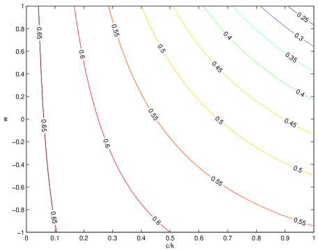
Figure 4: The value of the expansion rate $\lambda$ at which the attractor for the network’s evolution changes from a fixed charge solution to the standard linear scaling one, as a function of the parameters $w$ and $c/k$.

VIII Discussion and conclusions

We have extended the velocity-dependent one-scale string evolution model to the case where there is a conserved microscopic charge on the string worldsheet. We find that there are two possible regimes for the evolution of the network. When the expansion rate of the universe is fast enough the macroscopic charge will decay and the attractor solution is the standard linear scaling regime, where the network is losing energy as fast as is allowed by causality. When the expansion rate is relatively slow, the attractor solution has a constant macroscopic charge, with the defect velocities decreasing and the network correlation length growing more slowly than allowed by causality. However, even in this case, the network does not generically frustrate: the correlation length evolves more slowly than $\xi\propto t$ but faster than $\xi\propto a$ (conformal stretching); only in the limit of arbitrarily large charge would the conformal stretching behaviour be reached.

The rate of expansion at which the transition from charge domination to linear scaling occurs will depend on the dynamical processes acting on the network. A larger charge makes scaling harder, but cosmological expansion provides a damping term which tends to dilute the charge and overcome its influence on the dynamics. Further energy loss mechanisms facilitate scaling. Specifically, this critical expansion rate is given, in terms of the model parameters identified in the previous sections, by

$$\lambda=\frac{2}{3}\,\frac{1-(0.5+w)c/2k}{1+(0.5-w)c/3k}\,.$$ (126)

Without any losses the exponent is $2/3$ (corresponding to the matter-dominated era), and its dependence on the model parameters is illustrated in Fig. 4.

While our study was purely analytical, we should note that some numerical work already exists which, at least qualitatively, is in agreement with our results. Specifically, the aforementioned results of Battye et al. (2009); Battye and Pearson (2010), which suggest violations of scaling, rely on simulations which are nominally done in Minkowski space, although they have some effective numerical damping which probably mimics a fairly small (but non-zero) expansion rate. This therefore agrees with our results for low expansion rates, if one assumes that there are some effective charge losses. In that case our results predict that the scaling exponent for $\xi$ will decrease as the charge increases. However, we would further suggest that in a cosmological setting (that is, with a faster expansion rate), the network may still scale.

Interestingly, something like that kind of behaviour seems to emerge in more recent work Battye et al. (2011), in which apparent scaling deviations in Minkowski space (for a different model, again in two dimensions) are in fact eliminated by increasing the amount of damping. A more quantitative comparison between our analytic solutions and these numerical results would certainly be instructive but is not possible at this stage: it would require knowledge of the behaviour of the defect velocities in the simulations, and that is not provided in any of these works Battye et al. (2009); Battye and Pearson (2010); Battye et al. (2011).

In any case, our analysis highlights the point that results derived in Minkowski space may not necessarily apply to the case of an expanding universe; this has already been discussed, for example for the case of wiggly cosmic strings in Martins and Shellard (2006). Finally, our results are also relevant for the case of superconducting strings and vortons, but this case is left for future work.

References

- Vilenkin and Shellard (1994) A. Vilenkin and E. P. S. Shellard, Cosmic Strings and other Topological Defects (Cambridge University Press, Cambridge, U.K., 1994).
- Hindmarsh and Kibble (1995) M. B. Hindmarsh and T. W. B. Kibble, Rept.Prog.Phys. 58, 477 (1995), eprint hep-ph/9411342.
- Copeland et al. (2011) E. J. Copeland, L. Pogosian, and T. Vachaspati, Class.Quant.Grav. 28, 204009 (2011), eprint 1105.0207.
- Kibble (2004) T. W. B. Kibble (2004), eprint astro-ph/0410073.
- Jeannerot et al. (2003) R. Jeannerot, J. Rocher, and M. Sakellariadou, Phys. Rev. D68, 103514 (2003), eprint hep-ph/0308134.
- Burgess et al. (2001) C. P. Burgess, M. Majumdar, F. Quevedo, G. Rajesh, and R.-J. Zhang, JHEP 0107, 047 (2001), eprint hep-th/0105204.
- Sarangi and Tye (2002) S. Sarangi and S. H. H. Tye, Phys. Lett. B536, 185 (2002), eprint hep-th/0204074.
- Dvali and Vilenkin (2004) G. Dvali and A. Vilenkin, JCAP 0403, 010 (2004), eprint hep-th/0312007.
- Copeland et al. (2004) E. J. Copeland, R. C. Myers, and J. Polchinski, JHEP 06, 013 (2004), eprint hep-th/0312067.
- Pourtsidou et al. (2011) A. Pourtsidou, A. Avgoustidis, E. J. Copeland, L. Pogosian, and D. A. Steer, Phys.Rev. D83, 063525 (2011), eprint 1012.5014.
- Avgoustidis et al. (2011) A. Avgoustidis, E. J. Copeland, A. Moss, L. Pogosian, A. Pourtsidou, et al., Phys.Rev.Lett. 107, 121301 (2011), eprint 1105.6198.
- Copeland and Saffin (2005) E. J. Copeland and P. M. Saffin, JHEP 0511, 023 (2005), eprint hep-th/0505110.
- Urrestilla and Vilenkin (2008) J. Urrestilla and A. Vilenkin, JHEP 0802, 037 (2008), eprint 0712.1146.
- Hindmarsh and Saffin (2006) M. Hindmarsh and P. M. Saffin, JHEP 0608, 066 (2006), eprint hep-th/0605014.
- Sakellariadou and Stoica (2008) M. Sakellariadou and H. Stoica, JCAP 0808, 038 (2008), eprint 0806.3219.
- Tye et al. (2005) S.-H. Tye, I. Wasserman, and M. Wyman, Phys.Rev. D71, 103508 (2005), eprint astro-ph/0503506.
- Avgoustidis and Shellard (2008) A. Avgoustidis and E. P. S. Shellard, Phys.Rev. D78, 103510 (2008), eprint 0705.3395.
- Avgoustidis and Copeland (2010) A. Avgoustidis and E. J. Copeland, Phys.Rev. D81, 063517 (2010), eprint 0912.4004.
- Polchinski (2004) J. Polchinski, pp. 229–253 (2004), eprint hep-th/0412244.
- Witten (1985) E. Witten, Nucl.Phys. B249, 557 (1985).
- Callan and Harvey (1985) C. G. Callan and J. A. Harvey, Nucl.Phys. B250, 427 (1985).
- Davis and Shellard (1988) R. L. Davis and E. P. S. Shellard, Phys.Lett. B209, 485 (1988).
- Ganoulis and Lazarides (1989) N. Ganoulis and G. Lazarides, Nucl.Phys. B316, 443 (1989).
- Carter and Peter (1995) B. Carter and P. Peter, Phys.Rev. D52, 1744 (1995), eprint hep-ph/9411425.
- Brax et al. (2006) P. Brax, C. van de Bruck, A. Davis, and S. C. Davis, JHEP 0606, 030 (2006), eprint hep-th/0604198.
- Davis and Shellard (1989) R. L. Davis and E. P. S. Shellard, Nucl.Phys. B323, 209 (1989).
- Brandenberger et al. (1996) R. H. Brandenberger, B. Carter, A.-C. Davis, and M. Trodden, Phys.Rev. D54, 6059 (1996), eprint hep-ph/9605382.
- Martins and Shellard (1998a) C. J. A. P. Martins and E. P. S. Shellard, Phys. Rev. D57, 7155 (1998a), eprint hep-ph/9804378.
- Martins and Shellard (1998b) C. J. A. P. Martins and E. P. S. Shellard, Phys.Lett. B445, 43 (1998b), eprint hep-ph/9806480.
- Nunes et al. (2011) A. S. Nunes, A. Avgoustidis, C. J. A. P. Martins, and J. Urrestilla, Phys.Rev. D84, 063504 (2011), eprint 1107.2008.
- Vachaspati and Achucarro (1991) T. Vachaspati and A. Achucarro, Phys.Rev. D44, 3067 (1991).
- Martins and Shellard (1996a) C. J. A. P. Martins and E. P. S. Shellard, Phys. Rev. D53, 575 (1996a), eprint hep-ph/9507335.
- Martins and Shellard (1996b) C. J. A. P. Martins and E. P. S. Shellard, Phys. Rev. D54, 2535 (1996b), eprint [http://arXiv.org/abs]hep-ph/9602271.
- Martins and Shellard (2002) C. J. A. P. Martins and E. P. S. Shellard, Phys. Rev. D65, 043514 (2002), eprint [http://arXiv.org/abs]hep-ph/0003298.
- Martins et al. (2004) C. J. A. P. Martins, J. N. Moore, and E. P. S. Shellard, Phys. Rev. Lett. 92, 251601 (2004), eprint hep-ph/0310255.
- Battye et al. (2009) R. A. Battye, J. A. Pearson, S. Pike, and P. M. Sutcliffe, JCAP 0909, 039 (2009), eprint 0908.1865.
- Battye and Pearson (2010) R. A. Battye and J. A. Pearson, Phys.Rev. D82, 125001 (2010), eprint 1010.2328.
- Carter (1997) B. Carter (1997), eprint hep-th/9705172.
- Avgoustidis and Shellard (2005) A. Avgoustidis and E. P. S. Shellard, Phys. Rev. D71, 123513 (2005), eprint hep-ph/0410349.
- Kibble and Turok (1982) T. W. B. Kibble and N. Turok, Phys.Lett. B116, 141 (1982).
- Burden (1985) C. J. Burden, Phys.Lett. B164, 277 (1985).
- Kibble (1985) T. W. B. Kibble, Nucl. Phys. B252, 227 (1985).
- Battye et al. (2011) R. A. Battye, J. A. Pearson, and A. Moss, Phys.Rev. D84, 125032 (2011), eprint 1107.1325.
- Martins and Shellard (2006) C. J. A. P. Martins and E. P. S. Shellard, Phys.Rev. D73, 043515 (2006), eprint astro-ph/0511792.