Real dqds for the nonsymmetric tridiagonal eigenvalue problem

Abstract

We present a new transform triple dqds to help to compute the eigenvalues of a real tridiagonal matrix $C$ using real arithmetic. The algorithm uses the real dqds transform to shift by a real number and tridqds to shift by a complex conjugate pair. We present what seems to be a new criteria for splitting the current pair $L,U$. The algorithm rejects any transform which suffers from excessive element growth and then tries a new transform. Our numerical tests show that the algorithm is about 100 times faster than the Ehrlich-Aberth method of D. A. Bini, L. Gemignani and F. Tisseur. Our code is comparable in performance to a complex dqds code and is sometimes 3 times faster.

1 Introduction

The dqds algorithm was introduced in $1994$ in [7] as a fast and extremely accurate way to compute all the singular values of a bidiagonal matrix $B$. This algorithm implicitly performs the Cholesky LR iteration on the tridiagonal matrix $B^{T}B$ and it is used in LAPACK. However the dqds algorithm can also be regarded as executing, implicitly, the LR algorithm applied to any tridiagonal matrix with $1$’s on the superdiagonal. Our interest is in real matrices which may have complex conjugate pairs of eigenvalues. It is natural to try to retain real arithmetic and yet permit complex shifts of origin. Our analogue of the double shift QR algorithm of J. G. F. Francis [12] is the triple step dqds algorithm. The purpose of this paper is to explain why 3 steps are needed to derive the algorithm, to explain how we reject transforms with unacceptable element growth and to compare performance with some rival methods. Our conclusion is that this procedure is clearly the fastest method available at the present time.

We say nothing about the need for a tridiagonal eigensolver because this issue is admirably covered in Bini, Gemignani and Tisseur [1]. In fact many parts of [1] have been of great help to us. We also acknowledge the preliminary work on this problem by Z. Wu in [23].

We do not follow Householder conventions except that we reserve capital Roman letters for matrices. Section 2 describes other methods, Section 3 presents standard, but needed, material on LR, dqds, double shifts and the implicit L theorem. Section 4 develops our tridqds algorithm, Section 5 is our error analysis, Section 6 our splitting, deflation and shift strategy, and Section 7 presents our numerical tests using Matlab. Finally, Section 8 gives our conclusions and also our ideas about why tridqds is only one (important) ingredient for a procedure that must also provide condition numbers and eigenvectors.

2 Other methods

2.1 2 steps of LR = 1 step of QR

A frequent exercise for students is to show that for a symmetric positive definite tridiagonal matrix 2 steps of the LR (Cholesky) algorithm produces the same matrix as 1 step of the QR algorithm. Less well known is the article by H. Xu [24] which extends this result when the symmetric matrix is not positive definite. The catch here is that the LR transform, if it exists, does not preserve symmetry. The remedy is to regard similarities by diagonal matrices as “trivial”, always available, operations. Indeed, diagonal similarities cannot introduce zeros into a matrix. So, when successful, 2 steps os LR are diagonally similar to one step of QR. Even less well known is a short paper by J. Slemons [20] showing that for a tridiagonal matrix, not necessarily symmetric, 2 steps of of LR are diagonally equivalent to 1 step of HR, see [2]. Note that when symmetry disappears then QR is out of the running because it does not preserve the tridiagonal property.

The point of listing these results is to emphasize that 2 steps of LR gives twice as many shift opportunities as 1 step of QR or HR. Thus convergence can be more rapid with LR (or dqds) than with QR or HR. This is one of the reasons that dqds is faster than QR for computing singular values of bidiagonals. This extra speed is an additional bonus to the fundamental advantage that dqds delivers high relative accuracy in all the singular values. The one drawback to dqds, for bidiagonals, is that the singular values must be computed in monotone increasing order; QR allows the singular values to be found in any order.

In our case, failure is always possible and so there is no constraint on the order in which eigenvalues are found. The feature of having more opportunities to shift leads us to favor dqds over QR and HR. See the list of other methods which follows. We take up the methods in historical order and consider only those that preserve tridiagonal form.

2.2 Cullum’s complex QR algorithm

As part of a program that used the Lanczos algorithm to reduce a given matrix to tridiagonal form in [4], Jane Cullum used the fact that an unsymmetric tridiagonal matrix may always be balanced by a diagonal similarity transformation. She then observed that another diagonal similarity with $1$ or $i$ produces a symmetric, but complex, tridiagonal matrix to which the (complex) tridiagonal QR algorithm may be applied. The process is not backward stable because the relation

$$\cos^{2}\tau+\sin^{2}\tau=1$$

is not constraint on $|\cos\tau|$ and $|\sin\tau|$ when they are not real. Despite the possibility of breakdown the method proved satisfactory in practice. We have not used it in our comparisons because we are persuaded by 2.1 that it is out performed by the complex dqds algorithm, described below.

2.3 Liu’s HR algorithm

In [13] Alex Liu found a variation on the HR algorithm of Angelika Bunse-Gerstner that, in exact arithmetic, is guaranteed not to breakdown - but the price is a temporary increase in bandwith. This procedure has only been implemented in Maple and we do not include it in our comparison.

2.4 Complex dqds

In his thesis David Day [5] developed a Lanczos-style algorithm to reduce a general matrix to tridiagonal form and, as with Jane Cullum, needed a suitable algorithm to compute its eigenvalues. He knew of the effectiveness of dqds in the symmetric positive definite case and realized that dqds extends formally to any tridiagonal that admits triangular factorization. Without positivity the attractive property of achieving high relative accuracy disappears but, despite possible element growth, the error analysis for dqds persists: if the transform does not breakdown then tiny well chosen changes in the entries of input $L,U$ (giving $\widetilde{L},\widetilde{U}$) and output $\hat{L},\hat{U}$ (giving $\breve{L},\breve{U}$) produces an exact relation

$$\breve{L}\breve{U}=\widetilde{L}\widetilde{U}-\sigma I$$

with the given shift $\sigma$. See Section 5.1. The code uses complex arithmetic because of the possible presence of complex conjugate pairs of eigenvalues. We have wrapped David Day’s complex dqds code in a more sophisticated wrapper that chooses suitable shifts after rejecting a transform for excessive element growth.

2.5 Ehrlich-Aberth algorithm

This very careful and accurate procedure was presented by Bini, Gemignani and Tisseur in [1]. It finds the zeros of the characteristic polynomial $p(\cdot)$ and exploits the tridiagonal form to evaluate $p^{\prime}(z)/p(z)$ for any $z$. The polynomial solver improves a full set of approximate zeros at each step. Initial approximations are found using a divide-and-conquer procedure that delivers the eigenvalues of the top and bottom halves of the matrix $T$. The quantity $p^{\prime}(z)/p(z)$ is evaluated indirectly as $\left[\operatorname{trace}(zI-T)^{-1}\right]$ using a QR factorization of $zI-T$. Since $T$ is not altered there is no deflation to assist efficiency. Very careful tests exhibit the method’s accuracy - but it is very slow compared to both dqds-type algorithms.

3 LR and dqds

The reader is expected to have had some exposure to the QR and/or LR algorithms so we will be brief.

3.1 LU factorization

Any $n\times n$ matrix $A$ permits unique triangular factorization $A=LD\widetilde{U}$ where $L$ is unit lower triangular, $D$ is diagonal, $\widetilde{U}$ is unit upper triangular, if and only if the leading principal submatrices of orders $1,\dots,n-1$ are nonsingular.

In this paper we follow common practice and write $U=D\widetilde{U}$ so that the “pivots” (entries of $D$) lie on $U$’s diagonal. Throughout this paper any matrix $L$ is unit lower triangular and $U$ is upper triangular.

3.2 LR transform with shift

Note that $U$ is “right” triangular and $L$ is “left” triangular and this explains the standard name LR. For any shift $\sigma$ let

$$A-\sigma I =LU,$$ (1)

$$\widehat{A} =UL+\sigma I.$$ (2)

Then $\widehat{A}$ is the LR$(\sigma)$ transform of $A$. Note that

$$\widehat{A}=L^{-1}(A-\sigma I)L+\sigma I=L^{-1}AL.$$

We say that the shift is restored (in contrast to dqds - see below). The LR algorithm consists of repeated LR transforms with shifts chosen to enhance convergence to upper triangular form. For the theory see [18, 19, 21, 22].

In contrast to the well known QR algorithm, the LR algorithm can breakdown and can suffer from element growth, $\|L\|>>\|A\|$, $\|U\|>>\|A\|$. However LR preserves the banded form of $A$ while QR does not (except for the Hessenberg form).

When a matrix $A$ is represented by its entries then the shift operation $A\longrightarrow A-\sigma I$ is trivial. When a matrix is given in factored form the shift operation is not trivial.

3.3 The dqds algorithm

From now on we focus on tridiagonal matrices in $J$-form - entries $(i,i+1)$ are all $1$, $i=1,\ldots,n-1$. Throughout this paper all $J$ matrices have this form.

If $J-\sigma I$ permits triangular factorization

$$J-\sigma I=LU$$

then $L$ and $U$ must have the following form

$$\begin{array}[]{cc}L=\begin{bmatrix}1&&&&\\ l_{1}&1&&&\\ &\ddots&\ddots&&\\ &&l_{n-2}&1&\\ &&&l_{n-1}&1\end{bmatrix},&\qquad U=\begin{bmatrix}u_{1}&1&&&\\ &u_{2}&1&&\\ &&\ddots&\ddots&\\ &&&u_{n-1}&1\\ &&&&u_{n}\end{bmatrix}.\end{array}$$ (3)

It is an attractive feature of LR that

$$UL=\widehat{J}$$

is also of $J$-form. Thus the parameters $l_{i}$, $i=1,\ldots,n-1$, and $u_{j}$, $j=1,\ldots,n$, determine the matrices $L$ and $U$ above and implicitly define two tridiagonal matrices $LU$ and $UL$.

The qds algorithm is equivalent to the LR algorithm but no tridiagonal matrices are ever formed. The progressive transformation is from $L,U$ to $\widehat{L},\widehat{U}$,

$$\widehat{L}\widehat{U}=UL-\sigma I.$$ (4)

Notice that the shift is not restored and so $\widehat{U}\widehat{L}$ is not similar to $UL$.

Equating entries in each side of equation (4) gives

$$\begin{array}[]{rl}\textbf{{qds}}(\sigma):&\hat{u}_{1}=u_{1}+l_{1}-\sigma;\\ &\mbox{{for }}i=1,\ldots,n-1\\ &\hskip 17.07182pt\hat{l}_{i}=l_{i}u_{i+1}/\hat{u}_{i}\\ &\hskip 17.07182pt\hat{u}_{i+1}=u_{i+1}+l_{i+1}-\sigma-\hat{l}_{i}\\ &\mbox{{end for}}.\end{array}$$

The algorithm qds fails when $\hat{u}_{i}=0$ for some $i<n.$ When $\sigma=0$ we write simply qd, not qds.

In 1994 a better way was found to implement $\textsl{qds}(\sigma)$ that had been used by Rutishauser as early as 1955. These are called differential qd algorithms. See [15] for more history. This form uses uses an extra variable $d$ but has compensating advantages.

$$\begin{array}[]{rl}\textbf{{dqds}}(\sigma):&d_{1}=u_{1}-\sigma\\ &\mbox{{for }}i=1,\ldots,n-1\\ &\hskip 17.07182pt\hat{u}_{i}=d_{i}+l_{i}\\ &\hskip 17.07182pt\hat{l}_{i}=l_{i}(u_{i+1}/\hat{u}_{i})\\ &\hskip 17.07182ptd_{i+1}=d_{i}(u_{i+1}/\hat{u}_{i})-\sigma\\ &\mbox{{end for}}\\ &\hat{u}_{n}=d_{n}.\end{array}$$

By definition, dqd=dqds(0).

A word on terminology. In Rutishauser’s original work $q_{i}=u_{i}$, $e_{i}=l_{i}$; the $q_{i}$’s were certain quotients and and the $e_{i}$’s were called modified differences. In fact the qd algorithm led to the LR algorithm, not vice-versa. The reader can find more information concerning dqds in [15, 16]

One virtue of the dqds and QR transforms is that they work on the whole matrix so that large eigenvalues are converging near the top, albeit slowly, while the small ones are being picked off at the bottom.

We summarize some advantages and disadvantages of the factored form.

Advantages of the factored form

1. $L,U$ determines the entries of $J$ to greater than working-precision accuracy because the addition and multiplication of $l$’s and $u$’s is implicit. Thus, for instance, the $(i,i)$ entry of $J$ is given by $l_{i-1}+u_{i}$ implicitly but $fl(l_{i-1}+u_{i})$ explicitly.

2. Singularity of $J$ is detectable by inspection when $L$ and $U$ are given, but only by calculation from $J$. So, $LU$ reveals singularity, $J$ does not.

3. $LU$ defines the eigenvalues better than $J$ does (usually). There is more on this in [6].

4. Solution of $Jx=b$ takes half the time when $L$ and $U$ are available.

Disadvantages of the factored form

The mapping $J,\sigma\mapsto L,U$ is not everywhere defined for all pairs $J,\sigma$ and can suffer from element growth. This defect is not as serious as it was when the new transforms were written over the old ones. For tridiagonals we can afford to double the storage and map $L,U$ into different arrays $\widehat{L},\widehat{U}$. Then we can decide whether or not to accept $\widehat{L},\widehat{U}$ and only then would $L$ and $U$ be overwritten. So the difficulty of excessive element growth has been changed from disaster to the non-trivial but less intimidating one of, after rejecting a transform, choosing a new shift that will not spoil convergence and will not cause another rejection.

Now we turn to our main question of $\textsl{dqds}(\sigma)$: how can complex shifts be used without having to use complex arithmetic? This question has a beautiful answer for QR and LR iterations.

3.4 Double shift LR algorithm

We use the $J,L$ and $U$ notation from the previous section. Consider two steps of the LR algorithm with shifts $\sigma_{1}$ and $\sigma_{2}$,

$$J_{2}-\sigma_{1}I =L_{2}U_{2}$$

$$J_{3} =U_{2}L_{2}+\sigma_{1}I$$

$$J_{3}-\sigma_{2}I =L_{3}U_{3}$$

$$J_{4} =U_{3}L_{3}+\sigma_{1}I.$$

Then

$$J_{4}=\boldsymbol{\cal{L}}^{-1}J_{2}\boldsymbol{\cal{L}}$$ (5)

with

$$\boldsymbol{\cal{L}}=L_{2}L_{3},\quad\boldsymbol{\cal{U}}=U_{3}U_{2}$$

and

$$\boldsymbol{\cal{L}}\boldsymbol{\cal{U}} =L_{2}(J_{3}-\sigma_{2}I)U_{2}$$

$$=L_{2}(U_{2}L_{2}+\sigma_{1}I)U_{2}-\sigma_{2}L_{2}U_{2}$$

$$=L_{2}U_{2}\left[L_{2}U_{2}+(\sigma_{1}-\sigma_{2})I\right]$$

$$=(J_{2}-\sigma_{1}I)(J_{2}-\sigma_{2}I)$$

$$=J_{2}^{2}-(\sigma_{1}+\sigma_{2})J_{2}+\sigma_{1}\sigma_{2}I=:M$$ (6)

Suppose that $J_{2}$ is real and $\sigma_{1}$ is complex. Then $J_{4}$ will be real if, and only if, $\sigma_{2}=\bar{\sigma}$. The reason is that $M$ is real, so that $\boldsymbol{\cal{L}}$ and $\boldsymbol{\cal{U}}$ are real and, by (5), $J_{4}$ is the product of real matrices. Note however that $L_{2},U_{2},L_{3},U_{3}$ are all complex. Fortunately it is possible to compute $J_{4}$ from $J_{2}$ without using $J_{3}$. This depends on the following result.

Theorem 1.

[Implicit L theorem] If $H_{1}$ and $H_{2}$ are unreduced upper Hessenberg matrices and $H_{2}=L^{-1}H_{1}L$, where $L$ is unit lower triangular, then $H_{2}$ and $L$ are completely determined by $H_{1}$ and column 1 of $L$, $L\boldsymbol{e}_{1}$.

We omit the proof.

The clever application to $J_{2}$ and $J_{4}$ is to observe that column 1 of $M$,

$$M\boldsymbol{e}_{1}=\boldsymbol{\cal{L}}\boldsymbol{\cal{U}}\boldsymbol{e}_{1}=\boldsymbol{\cal{L}}\boldsymbol{e}_{1}u_{11},\quad u_{11}=m_{11},$$

is proportional to column 1 of $\mathbf{L}$ and has only three nonzero entries below the diagonal because $J_{2}$ is tridiagonal. Now choose

$$\mathcal{L}_{1}=I+\boldsymbol{m}\boldsymbol{e_{1}}^{T}$$

where

$$\boldsymbol{m}=\begin{bmatrix}0&m_{21}/m_{11}&m_{31}/m_{11}&0&\ldots&0\end{bmatrix}^{T}$$

and perform an explicit similarity transform on $J_{2}$,

$$\mathcal{L}_{1}^{-1}J_{2}\mathcal{L}_{1}=:K.$$

Observe that $K$ is not tridiagonal. In the $6\times 6$ case

$$K=\begin{bmatrix}x&1&&&&\\ x&x&1&&&\\ +&x&x&1&&\\ +&&x&x&1&\\ &&&x&x&1\\ &&&&x&x\end{bmatrix}.$$

Next we apply a sequence of elementary similarity transformations such that each transformation pushes the $2\times 1$ bulge one row down and one column to the right. Finally the bulge is chased off the bottom to restore the $J$-form. In exact arithmetic, the implicit L theorem ensures that this technique of bulge chasing gives

$$J_{4}=(\mathcal{L}_{1}\ldots\mathcal{L}_{n-1})^{-1}J_{2}(\mathcal{L}_{1}\ldots\mathcal{L}_{n-1})\;\;\text{ and }\;\;\boldsymbol{\cal{L}}=\mathcal{L}_{1}\ldots\mathcal{L}_{n-1}.$$

4 Triple dqds algorithm

4.1 Connection to LR algorithm

In figure 1 we examine the double shift LR transform derived in section 3.4 but with a significant difference. Instead of $J_{2}$ being an arbitrary real matrix in $J$-form, we assume that it is given to us in the form $U_{1}L_{1}$ obtained from one step of the LR algorithm with shift $0$ from real $J_{1}$.

Figure 1: Double shift LR and three steps of dqds

The crucial observation is that, along the bottom line $L_{2},U_{2},L_{3},U_{3}$ are all complex and so it requires 3 dqds steps to go from real $L_{1},U_{1}$ to real $L_{4},U_{4}$. Moreover the non-restoring shifts in dqds are

$$\sigma-0,\quad\bar{\sigma}-\sigma,\quad 0-\bar{\sigma}.$$

Here is another way of seeing the relation between LR and dqds:

$$\left\{\begin{array}[]{ll}J_{1}=&L_{1}U_{1}\\ J_{2}=&U_{1}L_{1}\end{array}\right.$$

$$\left\{\begin{array}[]{rll}J_{2}-\sigma I=&L_{2}U_{2}&\qquad L_{2}U_{2}=U_{1}L_{1}-\sigma I\\ J_{3}=&U_{2}L_{2}+\sigma I\end{array}\right.$$

$$\left\{\begin{array}[]{rll}J_{3}-\overline{\sigma}I=&L_{3}U_{3}&\qquad L_{3}U_{3}=(U_{2}L_{2}+\sigma I)-\overline{\sigma}I\\ J_{4}=&U_{3}L_{3}+\overline{\sigma}I\end{array}\right.$$

$$\left\{\begin{array}[]{rll}J_{4}=&L_{4}U_{4}&\qquad L_{4}U_{4}=(U_{3}L_{3}+\overline{\sigma}I)-0I\\ \ldots&\phantom{J_{4}=U_{3}L_{3}+\overline{\sigma}I}\end{array}\right.$$

Recall from the previous section that the double LR algorithm can work with complex shifts in real arithmetic by bulge chasing. The rest of this section developes a form of bulge chasing for the dqds algorithm.

4.2 3 steps of dqds

In contrast to a single dqds step our triple dqds restores the shifts. Recall from (5) in section 3.4 that

$$L_{4}U_{4}=J_{4}=\boldsymbol{\cal{L}}^{-1}J_{2}\boldsymbol{\cal{L}}=\boldsymbol{\cal{L}}^{-1}U_{1}L_{1}\boldsymbol{\cal{L}}$$ (7)

and, since $\sigma_{1}=\sigma\text{ and }\sigma_{2}=\bar{\sigma}$, matrix $M$ in (6) is given by

$$M=(U_{1}L_{1})^{2}-2(\Re\sigma_{1})U_{1}L_{1}+|\sigma_{1}|^{2}I.$$ (8)

The idea is to transform $U_{1}$ into $L_{4}$ and $L_{1}$ into $U_{4}$ by bulge chasing in each matrix,

$$L_{4}U_{4}=\underbrace{\boldsymbol{\cal{L}}^{-1}U_{1}}\underbrace{L_{1}\boldsymbol{\cal{L}}}.$$

Notice that we need to transform an upper bidiagonal into a lower bidiagonal and vice-versa. From the uniqueness of the $LU$ factorization, when it exists, it follows that there is a unique hidden matrix $X$ such that

$$L_{4}=\boldsymbol{\cal{L}}^{-1}U_{1}X^{-1},\quad XL_{1}\boldsymbol{\cal{L}}=U_{4}.$$

For more on $X$ see [14]. The matrix $\boldsymbol{\cal{L}}$ is given, from section 3.4 as a product

$$\boldsymbol{\cal{L}}=\mathcal{L}_{1}\ldots\mathcal{L}_{n-1}\mathcal{L}_{n}$$

($\mathcal{L}_{n}=I$) and we will gradually construct the matrix $X$ in corresponding factored form $X_{n},\ldots,X_{2}X_{1}$. In fact we will write each $X_{i}$ as a product

$$X_{i}=Y_{i}Z_{i}.$$

The details are quite complicated.

4.2.1 Chasing the bulges

Starting with the factors $L_{1}$, $U_{1}$ and the shift $\sigma$, we normalize column 1 of $M$ in (8) to form ${\mathcal{L}}_{1}$, spoil the bidiagonal form with

$$\underbrace{\mathcal{L}_{1}^{-1}U_{1}}\underbrace{L_{1}\mathcal{L}_{1}}$$

and at each minor step $i$, $i=1,\ldots,n$, matrices $Z_{i}$, $\mathcal{L}_{i}$ and $Y_{i}$ are chosen to chase the bulges. After $n$ minor steps, we obtain $L_{4}$ and $U_{4}$,

$$L_{4}U_{4}= \underbrace{\mathcal{L}_{n}^{-1}\cdots\mathcal{L}_{1}^{-1}U_{1}Z_{1}^{-1}Y_{1}^{-1}\cdots Z_{n}^{-1}Y_{n}^{-1}}\underbrace{Y_{n}Z_{n}\cdots Y_{1}Z_{1}L_{1}\mathcal{L}_{1}\cdots\mathcal{L}_{n}}$$

$$= \underbrace{\mathcal{L}_{n}^{-1}\cdots\mathcal{L}_{1}^{-1}U_{1}X_{1}^{-1}\cdots X_{n}^{-1}}\underbrace{X_{n}\cdots X_{1}L_{1}\mathcal{L}_{1}\cdots\mathcal{L}_{n}}$$

$$= \underbrace{\boldsymbol{\cal{L}}^{-1}U_{1}X^{-1}}\underbrace{XL_{1}\boldsymbol{\cal{L}}}$$

Conceptually we create two work arrays $F$ and $G$. Initially,

$$F=U_{1},\qquad G=L_{1}$$

and, finally,

$$F=L_{4},\qquad G=U_{4}.$$

For a complex shift $\sigma$, the triple dqds algorithm has the following matrix formulation:

$$\begin{array}[]{rll}\textbf{{tridqds}}(\sigma,\bar{\sigma}):&\\ &F=U_{1};\;G=L_{1}\\ &F=FZ_{1}^{-1};\;G=Z_{1}G\\ &F=\mathcal{L}_{1}^{-1}F;\;G=G\mathcal{L}_{1}&[\text{form }\mathcal{L}_{1}\text{ using }(\ref{M3dqds})]\\ &F=FY_{1}^{-1};\;G=Y_{1}G\\ \\ &\textbf{for }i=2,\ldots,n-3\\ &\hskip 17.07182ptF=FZ_{i}^{-1};\;G=Z_{i}G\\ &\hskip 17.07182ptF=\mathcal{L}_{i}^{-1}F;\;G=G\mathcal{L}_{i}\\ &\hskip 17.07182ptF=FY_{i}^{-1};\;G=Y_{i}G&[Z_{i}\text{ with one, }\mathcal{L}_{i}\text{ with two and }Y_{i}\text{ with three}\\ &\textbf{end for}&\text{\;nonzero off-diagonal entries}]\\ \\ &\textsf{\% \;\;\text{step } n-2}\\ &F=FZ_{n-2}^{-1};\;G=Z_{n-2}G\\ &F=\mathcal{L}_{n-2}^{-1}F;\;G=G\mathcal{L}_{n-2}\\ &F=FY_{n-2}^{-1};\;G=Y_{n-2}G&[Y_{n-2}\text{ with two nonzero off-diagonal entries}]\\ \\ &\textsf{\%\;\;\text{step } n-1}\\ &F=FZ_{n-1}^{-1};\;G=Z_{n-1}G\\ &F=\mathcal{L}_{n-1}^{-1}F;\;G=G\mathcal{L}_{n-1}\\ &F=FY_{n-1}^{-1};\;G=Y_{n-1}G&[Y_{n-1}\text{ and }\mathcal{L}_{n-1}\text{ with one nonzero off-diagonal entry}]\\ \\ &\textsf{\%\;\;\text{step } n}\\ &\mathcal{L}_{n}=I;\;Y_{n}=I\\ &F=FZ_{n}^{-1};\;G=Z_{n}G&[Z_{n}\text{ diagonal}]\\ &L_{4}=F;\;F_{4}=G\end{array}$$

4.2.2 Details of tridqds

In this section we will go into the details of the tridqds algorithm described in the previous section. Consider $L_{1}$ with subdiagonal entries $\l_{1},\ldots,l_{n-1}$ and $U_{1}$ with diagonal entries $u_{1},\ldots,u_{n}$, as defined in Section 3.3, and consider matrices $L_{4}$ and $U_{4}$ with subdiagonal entries $\hat{l}_{1},\ldots,\hat{l}_{n-1}$ and diagonal entries $\hat{u}_{1},\ldots,\hat{u}_{n}$, respectively.

For each iteration of tridqds, at the beginning of a minor step $i,\;i=2,\ldots,n-2,$ the active $4\times 4$ windows of $F$ and $G$ are

$$F=\begin{bmatrix}\ddots&&&&&\\ \ddots&1&&&&\\ &\hat{l}_{i-1}&u_{i}&1&&\\ &+&&u_{i+1}&1&\\ &+&&&u_{i+2}&\ddots\\ &&&&&\ddots\end{bmatrix},\qquad G=\begin{bmatrix}\ddots&\ddots&&&&\\ &\hat{u}_{i-1}&1&&&\\ &&*&&&\\ &&+&1&&\\ &&+&l_{i+1}&1&\\ &&&&\ddots&\ddots\end{bmatrix}.$$ (9)

Each minor step $i$, $i=2,\ldots,n-3$, consists of the following 3 parts.

$\underline{\textbf{Minor step {i}}}$

• $F\longleftarrow FZ_{i}^{-1}$ puts 0 into $F_{i,i+1}$ and 1 into $F_{i,i}$

  $G\longleftarrow Z_{i}G$ turns $G_{i,i+1}$ into 1

  $$Z_{i}^{-1}=\begin{bmatrix}\ddots&&&&&\\ &1&&&&\\ &&\frac{1}{u_{i}}&-\frac{1}{u_{i}}&&\\ &&0&1&&\\ &&&&1&\\ &&&&&\ddots\\ \end{bmatrix},\qquad\qquad Z_{i}=\begin{bmatrix}\ddots&&&&&\\ &1&&&&\\ &&u_{i}&1&&\\ &&0&1&&\\ &&&&1&\\ &&&&&\ddots\end{bmatrix},$$

  $$FZ_{i}^{-1}=\begin{bmatrix}\ddots&&&&&\\ \ddots&1&&&&\\ &\hat{l}_{i-1}&1&0&&\\ &+&&u_{i+1}&1&\\ &+&&&u_{i+2}&\ddots\\ &&&&&\ddots\end{bmatrix},\;\;\;\;Z_{i}G=\begin{bmatrix}\ddots&\ddots&&&&\\ &\hat{u}_{i-1}&1&&&\\ &&*&1&&\\ &&+&1&&\\ &&+&l_{i+1}&1&\\ &&&&\ddots&\ddots\end{bmatrix}.$$

• $F\longleftarrow\mathcal{L}_{i}^{-1}F$ puts 0 in $F_{i+1,i-1}$ and $F_{i+2,i-1}$

  $G\longleftarrow G\mathcal{L}_{i}$ defines $\hat{u}_{i}$ and creates 3 nonzeros below it

  $$\mathcal{L}_{i}^{-1}=\begin{bmatrix}\ddots&&&&&\\ &\ddots&&&&\\ &&1&&&\\ &&*&1&&\\ &&*&&1&\\ &&&&&\ddots\end{bmatrix}=I+\boldsymbol{x}\boldsymbol{e}_{i}^{T},\qquad\qquad\mathcal{L}_{i}=I-\boldsymbol{x}\boldsymbol{e}_{i}^{T},$$

  $$\mathcal{L}_{i}^{-1}F=\begin{bmatrix}\ddots&&&&&\\ \ddots&1&&&&\\ &\hat{l}_{i-1}&1&&&\\ &&*&u_{i+1}&1&\\ &&+&&u_{i+2}&1\\ &&&&&\ddots\end{bmatrix},\;\;\;G\mathcal{L}_{i}=\begin{bmatrix}\ddots&\ddots&&&&\\ &\hat{u}_{i}&1&&\\ &+&1&&\\ &+&l_{i+1}&1&\\ &+&&l_{i+2}&1\\ &&&&\ddots&\ddots\end{bmatrix}.$$

• $G\longleftarrow Y_{i}G$ puts 0 in $G_{i+1,i}$, $G_{i+2,i}$ and $G_{i+3,i}$

  $F\longleftarrow FY_{i}^{-1}$ creates $\hat{l}_{i}$ and puts 2 nonzeros below it

  $$Y_{i}^{-1}=\begin{bmatrix}\ddots&&&&&\\ &1&&&\\ &*&1&&\\ &*&&1&\\ &*&&&1\\ &&&&&\ddots\end{bmatrix}=I+\boldsymbol{y}\boldsymbol{e}_{i}^{T},\qquad\qquad Y_{i}=I-\boldsymbol{y}\boldsymbol{e}_{i}^{T},$$

  $$FY_{i}^{-1}=\begin{bmatrix}\ddots&&&&&\\ \ddots&1&&&&\\ &\hat{l}_{i}&u_{i+1}&1&&\\ &+&&u_{i+2}&1&\\ &+&&&u_{i+3}&\ddots\\ &&&&&\ddots\end{bmatrix},\;\;Y_{i}G=\begin{bmatrix}\ddots&\ddots&&&&\\ &\hat{u}_{i}&1&&&\\ &&*&&&\\ &&+&1&&\\ &&+&l_{i+2}&1&\\ &&&&\ddots&\ddots\end{bmatrix}.$$

The result of this minor step is that the active windows of $F$ and $G$ shown in (9) have been moved down and to the right by one place. See Appendix A for more details on the practical implementation.

Naturally steps $1,n-2,n-1,n$ are slightly different and may be found on pp. 147-157 of [8].

4.3 Operation count for tridqds

In this section we will see how three steps of simple dqds algorithm compares with one step of tridqds in what respects to the number of floating point operations required.

Here is the inner loop of tridqds. See Appendix B.

$$\begin{array}[]{rll}\textbf{{tridqds}}(\sigma,\bar{\sigma}):&\\ &\textbf{for }i=2,\ldots,n-3\\ &\hskip 17.07182ptx_{r}=x_{r}*u_{i}+y_{r}\\ &\hskip 17.07182ptx_{l}=-x_{l}*(1/\hat{l}_{i-1});\;\;y_{l}=-y_{l}*(1/\hat{l}_{i-1});\\ &\hskip 17.07182pt\hat{u}_{i}=x_{r}-x_{l};\\ &\hskip 17.07182ptx_{r}=y_{r}-x_{l};\;\;y_{r}=z_{r}-y_{l}-x_{l}*l_{i+1};\;\;z_{r}=-y_{l}*l_{i+2}\\ &\hskip 17.07182ptx_{r}=x_{r}*(1/\hat{u}_{i});\;\;y_{r}=y_{r}*(1/\hat{u}_{i});\;\;z_{r}=z_{r}*(1/\hat{u}_{i})\\ &\hskip 17.07182pt\hat{l}_{i}=x_{l}+y_{r}+x_{r}*u_{i+1}\\ &\hskip 17.07182ptx_{l}=y_{l}+z_{r}+y_{r}*u_{i+2};\;\;y_{l}=z_{r}*u_{i+3}\\ &\hskip 17.07182ptx_{r}=1-x_{r};\;\;y_{r}=l_{i+1}-y_{r};\;\;z_{r}=-z_{r}\\ &\textbf{end for}\\ \end{array}$$

A good compiler recognizes common subexpressions.

In contrast,

$$\begin{array}[]{rl}\textbf{{dqds}}(\sigma):&d_{1}=u_{1}-\sigma\\ &\mbox{{for }}i=1,\ldots,n-1\\ &\hskip 17.07182pt\hat{u}_{i}=d_{i}+l_{i}\\ &\hskip 17.07182pt\hat{l}_{i}=l_{i}(u_{i+1}/\hat{u}_{i})\\ &\hskip 17.07182ptd_{i+1}=d_{i}(u_{i+1}/\hat{u}_{i})-\sigma\\ &\mbox{{end for}}\\ &\hat{u}_{n}=d_{n}.\end{array}$$

In practice, each $d_{i+1}$ may be written over its predecessor in a single variable $d$ and, if the common subexpression $u_{i+1}/\hat{u}_{i}$ is recognized, then only one division is needed if we use an auxiliary variable.

Table 1 below shows that the operation count of one step of tridqds is comparable to three steps of dqds (table expresses only the number of floating point operations in the inner loops).

	tridqds	3 dqds steps
Divisions	2	3
Multiplications	11	6
Additions	5	3
Subtractions	6	3
Assignments	16	12
Auxiliary variables	5	2

Table 1: Operation count of tridqds and 3 dqds steps

But to make three steps of dqds equivalent to tridqds we have to consider dqds in complex arithmetic and the total cost is raised by a factor of about 4. Thus, in complex arithmetic, three steps of dqds are much more expensive than one step of tridqds.

5 Error analysis

We turn to the effect of finite precision arithmetic on our algorithms. First consider the dqds algorithm.

5.1 dqds

In the absence of over/underflow the algorithm enjoys the so-called mixed relative stability property.

Theorem 2.

Let $\textsl{dqds}(\sigma)$ map $L,U$ into computed $\widehat{L},\widehat{U}$ with no division by zero, over/underflow. Then well chosen small relative changes in the entries of both input and output matrices, of at most 3 ulps each, produces new matrices, one pair mapped into the other, in exact arithmetic, by $\textsl{dqds}(\sigma)$.

See the diagram in Figure 2. The remarkable feature here is that huge element growth does not impair the result. However this useful property does not guarantee that dqds returns accurate eigenvalues. See [7, 15]. For that, an extra requirement is needed such as positivity of all the parameters $u_{j}$, $l_{j}$ in the computation. This is the case for the eigenvalues of $B^{T}B$ where $B$ is upper bidiagonal.

What can be said in our case? We quote a result that is established by Yao Yang in his dissertation [25] and appears in [15]. The clever idea is not to look at the $L$ and $U$ separately but to study their exact product $J=LU$.

$$\begin{CD}{L,U}@>{\operatorname{\hskip 14.22636ptdqds\hskip 14.22636pt}}>{\operatorname{computed}}>{\widehat{L},\widehat{U}}\\ @V{\operatorname{\scriptsize{\begin{array}[]{l}\text{change each}\\ l_{k}\text{ by 1 ulp}\\ u_{k}\text{ by 3 ulps}\\ \end{array}}}}V{}V@A{}A{\operatorname{\scriptsize{\begin{array}[]{l}\text{change each}\\ \breve{l}_{k},\;\breve{u}_{k}\text{ by 2 ulps}\\ \end{array}}}}A\\ {\widetilde{L},\widetilde{U}}@>{\operatorname{\hskip 14.22636ptdqds\hskip 14.22636pt}}>{\operatorname{exact}}>{\breve{L},\breve{U}}\end{CD}$$

$\breve{L}\breve{U}=\widetilde{U}\widetilde{L}-\sigma I$

Figure 2: Effects of roundoff for dqds

Theorem 3.

[Y. Yang] If $\textsl{dqds}(\sigma)$ maps $L,U$ into $\widehat{L},\widehat{U}$ (with no division by 0, overflow/underflow) in the standard model of floating point arithmetic then there is a unique pair $\mathring{L},\mathring{U}$ such that, in exact arithmetic, $\textsl{dqds}(\sigma)$ maps $\mathring{L},\mathring{U}$ into $\widehat{L},\widehat{U}$. Moreover, the associated tridiagonals satisfy, element by element,

$$|\operatorname{offdiag}(\mathring{J})-\operatorname{offdiag}(J)|<2\varepsilon|\operatorname{offdiag}(J)|$$

$$|\mathop{\operator@font diag}\nolimits(\mathring{J})-\mathop{\operator@font diag}\nolimits(J)|<\varepsilon\left(2|\boldsymbol{u}|+|\sigma||\boldsymbol{1}|+|\boldsymbol{\hat{l}}|+|\boldsymbol{\hat{u}}|+2|\boldsymbol{d}|\right)$$

where $\varepsilon$ is the roundoff unit.

This result is Corollary 3 in Section 9 of [15]. It shows that it is only the diagonal of $J$ that suffers large backward error in the case of element growth. Since $\boldsymbol{\hat{u}}=\boldsymbol{d}+\boldsymbol{\hat{l}}$ the last inequality may be written as

$$|\mathop{\operator@font diag}\nolimits(\mathring{J})-\mathop{\operator@font diag}\nolimits(J)|<\varepsilon\left(2|\boldsymbol{u}|+|\boldsymbol{l}|+|\sigma||\boldsymbol{1}|+|\boldsymbol{\hat{l}}|+3|\boldsymbol{d}|\right).$$

Recall that $d_{i}^{-1}=\left[(UL)^{-1}\right]_{ii},\;i=1,\ldots,n$. Thus the indices vulnerable to large backward error belong to any very small entries $\left[(UL)^{-1}\right]_{ii}$. For this reason we reject $\widehat{L},\widehat{U}$ when, element by element,

$$|\sigma||\boldsymbol{1}|+|\boldsymbol{\hat{l}}|+3|\boldsymbol{d}|>1000(|\boldsymbol{u}|+|\boldsymbol{l}|).$$ (10)

Recall that the error analysis is worst case. Recall also that the effect of a tiny $\hat{u}_{k}$ disappears for $i>k+1$.

5.2 tridqds

There are too many intermediate variables in this algorithm to permit a successful mixed error analysis. However each minor step in the algorithm consists of 3 elementary similarity transformations on work matrices $F,G$ or $G,F$. See … in Section 4.2.1. Recall that an elementary matrix here is of the form $I+\boldsymbol{v}\boldsymbol{e}_{j}^{T}$, with inverse $I-\boldsymbol{v}\boldsymbol{e}_{j}^{T}$, and $\boldsymbol{v}$ has at most 3 nonzero entries. So we examine the condition number of these 3 similarity transforms. Consult Appendix A to follow the details.

• The active part of $Z_{i}$ is

  $$\begin{bmatrix}u_{i}&1\\ 0&1\end{bmatrix}\qquad\text{and}\qquad\operatorname{cond}(Z_{i})\simeq\max\left\{|u_{i}|,|u_{i}|^{-1}\right\}.$$

• The active part of $\mathcal{L}_{i}$ is

  $$\begin{bmatrix}1&\\ -x_{l}/\hat{l}_{i-1}&1\\ -y_{l}/\hat{l}_{i-1}&0&1\end{bmatrix}\qquad\text{and}\qquad\operatorname{cond}(\mathcal{L}_{i})\simeq 1+\left(\frac{x_{l}}{\hat{l}_{i-1}}\right)^{2}+\left(\frac{y_{l}}{\hat{l}_{i-1}}\right)^{2}.$$

• The active part of $Y_{i}$ is

  $$\begin{bmatrix}1&\\ -x_{r}/\hat{u}_{i}&1\\ -y_{r}/\hat{u}_{i}&0&1\\ -z_{r}/\hat{u}_{i}&0&0&1\\ \end{bmatrix}\qquad\text{and}\qquad\operatorname{cond}({Y}_{i})\simeq 1+\left(\frac{x_{r}}{\hat{u}_{i}}\right)^{2}+\left(\frac{y_{r}}{\hat{u}_{i}}\right)^{2}+\left(\frac{z_{r}}{\hat{u}_{i}}\right)^{2}.$$

The variables $x_{l},y_{l},x_{r},y_{r},z_{r}$ are formed from additions and multiplications of previous quantities. Note that $u_{i}$ is part of the input and so is assumed to be of acceptable size. We see that it is tiny values of $\hat{l}_{i-1}$ and $\hat{u}_{i}$ that lead to an ill-conditioned similarity at minor step $i$. In the simple dqds algorithm a small value of $\hat{u}_{i}$ (relative to $u_{i+1}$) leads to a large value of $\hat{l}_{i+1}$ and $d_{i+1}$. In tridqds the effect of 3 consecutive transforms is more complicated. The message is the same: reject any transform that has more then modest element growth, as determined by (10) in the previous section. This challenge calls for further study.

6 Implementation details

6.1 Deflation $\boldsymbol{(n\leftarrow n-1)}$

Some of out criteria for deflating come from [16], others are new. Consider both matrices $UL$ and $LU$ and the trailing $2\times 2$ blocks,

$$\begin{bmatrix}l_{n-1}+u_{n-1}&1\\ l_{n-1}u_{n}&u_{n}\end{bmatrix},\qquad\qquad\begin{bmatrix}l_{n-2}+u_{n-1}&1\\ l_{n-1}u_{n-1}&l_{n-1}+u_{n}\end{bmatrix}.$$

Deflation $(n\leftarrow n-1)$ removes $l_{n-1}$ as well as $u_{n}$. Looking at entry $(n-1,n-1)$ of $UL$ shows that a necessary condition is that $l_{n-1}$ be negligible compared to $u_{n-1}$,

$$|l_{n-1}|<tol\cdot|u_{n-1}|,$$ (11)

for a certain tolerance $tol$ close to roundoff unit $\varepsilon$.

The $(n,n)$ entries of $UL$ and $LU$ suggest either $u_{n}+Acshift$ or $l_{n-1}+u_{n}+Acshift$ as eigenvalues. $Acshift$ is the accumulated shift (recall that dqds is a non-restoring transform). To make these consistent we require that

$$|l_{n-1}|<tol\cdot|u_{n}+Acshift|.$$ (12)

Finally we must consider the change $\delta\lambda$ in the eigenvalue $\lambda$ caused by setting $l_{n-1}=0$. We estimate $\delta\lambda$ by starting from $UL$ with $l_{n-1}=0$ and then allowing $l_{n-1}$ to grow. To this end let $J$ be $UL$ with $l_{n-1}=0$ and $(u_{n},\boldsymbol{y}^{T},\boldsymbol{x})$ be the eigentriple for $J$. Clearly $\boldsymbol{y}^{T}=\boldsymbol{e}_{n}^{T}$. Now we consider perturbation theory with parameter $l_{n-1}$. The perturbing matrix $\delta J$, as $l_{n-1}$ grows, is

$$l_{n-1}(\boldsymbol{e}_{n-1}+\boldsymbol{e}_{n}u_{n})\boldsymbol{e}_{n-1}^{T}.$$

By first order perturbation analysis

$$|\delta\lambda|=\frac{|\boldsymbol{y}^{T}\delta J\boldsymbol{x}|}{\|\boldsymbol{x}\|_{2}\|\boldsymbol{y}\|_{2}}$$

and $\|\boldsymbol{y}\|_{2}=1$ in our case. So,

$$|\delta\lambda|=\frac{\left|l_{n-1}\boldsymbol{e}_{n}^{T}(\boldsymbol{e}_{n-1}+\boldsymbol{e}_{n}u_{n})\boldsymbol{e}_{n-1}^{T}\boldsymbol{x}\right|}{\|\boldsymbol{x}\|_{2}}=\frac{|l_{n-1}u_{n}||x_{n-1}|}{\|\boldsymbol{x}\|_{2}}$$

and we use the crude bound $\displaystyle\frac{|x_{n-1}|}{\|\boldsymbol{x}\|_{2}}<1.$ So, we let $l_{n-1}$ grow until the change

$$|\delta\lambda|<|l_{n-1}u_{n}|$$

in eigenvalue $\lambda=u_{n}$ is no longer acceptable. Our condition for deflation is then

$$|l_{n-1}u_{n}|<tol\cdot|Acshift+u_{n}|.$$ (13)

A similar first order perturbation analysis for $LU$ with $l_{n-1}=0$ will give our last condition for deflation. For the eigentriple $(u_{n},\boldsymbol{y}^{T},\boldsymbol{x})$ we also have $\boldsymbol{y}^{T}=\boldsymbol{e}_{n}^{T}$. The perturbing matrix is now

$$l_{n-1}\boldsymbol{e}_{n}\left(\boldsymbol{e}_{n-1}^{T}u_{n-1}+\boldsymbol{e}_{n}^{T}\right)$$

and

$$|\delta\lambda|=\frac{\left|l_{n-1}\boldsymbol{e}_{n}^{T}\boldsymbol{e}_{n}(\boldsymbol{e}_{n-1}^{T}u_{n-1}+\boldsymbol{e}_{n}^{T})\boldsymbol{x}\right|}{\|\boldsymbol{x}\|_{2}}=|l_{n-1}|\frac{|u_{n-1}x_{n-1}+x_{n}|}{\|\boldsymbol{x}\|_{2}}<|l_{n-1}|\left(|u_{n-1}|+1\right).$$

Finally we require

$$|l_{n-1}|\left(|u_{n-1}|+1\right)<tol\cdot|Acshift+u_{n}|.$$ (14)

6.2 Splitting and deflation $\boldsymbol{(n\leftarrow n-2)}$

Recall that the implicit L theorem was invoked to justify the tridqds algorithm. This result fails if any $l_{k}$, $k<n-1$ vanishes. Consequently, checking for negligible values among the $l_{k}$ is a necessity, not a luxury for increased efficiency. Consider $J=UL$ in block form

$$\left[\vbox{\hbox{\kern-1.1563pt\raise 0.0pt\hbox{\kern 29.63939pt}\kern 0.0pt\vbox{}\kern-1.1563pt}}\right]$$

where $\mu=u_{k+1}l_{k}$, $k<n-1$. We can replace $\mu$ by $0$ when

$$\operatorname{spectrum}(J_{1})\cup\operatorname{spectrum}(J_{2})=\operatorname{spectrum}(J),\quad\textsl{to working accuracy}.$$

However we are not going to estimate the eigenvalues of $J_{1}$ and $J_{2}$. Instead we create a local criterion for splitting at $(k+1,k)$ as follows. Focus on the principal $4\times 4$ window of $J$ given by

$$\left[\vbox{\hbox{\kern-1.1563pt\raise 0.0pt\hbox{\kern 138.30936pt}\kern 0.0pt\vbox{}\kern-1.1563pt}}\right].$$

Now $J_{1}$ and $J_{2}$ are both $2\times 2$ and our local criterion is

$$\det(J_{1})\cdot\det(J_{2})=\det(J),\quad\textsl{to working accuracy}.$$ (15)

Let us see what this yields. Perform block factorization on $J$ and note that the Schur complement of $J_{1}$ in $J$ is

$$J_{2}^{\prime}=J_{2}-\begin{bmatrix}0&\mu\\ 0&0\end{bmatrix}J_{1}^{-1}\begin{bmatrix}0&0\\ 1&0\end{bmatrix}$$

with

$$J_{1}^{-1} =\frac{1}{det_{1}}\begin{bmatrix}u_{k}+l_{k}&-1\\ -u_{k}l_{k-1}&u_{k-1}+l_{k-1}\end{bmatrix}$$

where

$$det_{1}=\det(J_{1})=u_{k-1}(u_{k}+l_{k})+l_{k-1}l_{k}.$$

Thus

$$J_{2}^{\prime}=\begin{bmatrix}u_{k+1}l_{k}&u_{k+1}+l_{k+1}\\ u_{k+2}l_{k+1}&u_{k+2}+l_{k+2}\end{bmatrix}-\begin{bmatrix}\mu(u_{k-1}+l_{k-1})/det_{1}&0\\ 0&0\end{bmatrix}.$$

Since $\det$ is linear by rows

$$\det(J_{2})-\det(J_{2}^{\prime})=\mu(u_{k-1}+l_{k-1})(u_{k+2}+l_{k+2})/det_{1}.$$

Our criterion reduces to splitting only when

$$\det(J_{2}^{\prime})=\det(J_{2}),\quad\text{to working accuracy}.$$

Thus we require

$$|l_{k}u_{k+1}(u_{k+2}+l_{k+2})(u_{k-1}+l_{k-1})/det_{1}|<tol\cdot\left|\det(J_{2})\right|.$$

Since

$$det_{2}=\det(J_{2})=u_{k+1}(u_{k+2}+l_{k+2})+l_{k+1}l_{k+2},$$

the criterion for splitting $J$ at $(k+1,k)$ is then

$$|l_{k}u_{k+1}(u_{k+2}+l_{k+2})(u_{k-1}+l_{k-1})|<tol\cdot\left|det_{1}det_{2}\right|.$$ (16)

Finally, to remove $l_{k}$ we also need $l_{k}$ to be negligible compared to $u_{k}$,

$$|l_{k}|<tol\cdot|u_{k}|.$$ (17)

Deflation $\boldsymbol{(n\leftarrow n-2)}$

We use the same criterion for deflation $(n\leftarrow n-2)$, but because $l_{k+2}=l_{n}=0$ there is a common factor $det_{2}$ on each side of (16). Deflate the trailing $2\times 2$ submatrix when

$$|l_{n-2}|<tol\cdot|u_{n-2}|$$ (18)

and

$$|l_{n-2}(u_{n-3}+l_{n-3})|<tol\cdot\left|u_{n-3}(u_{n-2}+l_{n-2})+l_{n-3}l_{n-2}.\right|.$$ (19)

We omit the role of $Acshift$ here because it makes the situation more complicated. We have to recall that tridqds uses restoring shifts and $Acshift$ is always real. So, for complex shifts, $det_{2}$ is not going to zero. In fact

$$|det_{2}|\geq|\Im(\lambda)|^{2}$$

where $\lambda$ is an eigenvalue of $J_{2}$.

When $n=3$ these criteria simplify a lot. Both reduce to

$$|l_{1}|<tol\cdot|u_{1}|.$$

6.3 Shift strategy

Although tridqds may be, and has been, used to compute all the eigenvalues, it seems sensible to include real $\textsl{dqds}(\sigma)$ so that when all eigenvalues are real tridqds need not be called.

As with LR, the dqds algorithm with no shift gradually forces large entries to the top and brings small entries towards the bottom. Before every transform both $l_{n-1}$ and $l_{n-2}$ are inspected. If

$$|l_{n-1}|<\frac{1}{2^{4}}\qquad\text{and}\qquad|l_{n-2}|<\frac{1}{2^{4}}$$

then the code executes dqds transform with the Wilkinson shift or a 3dqds transform with Francis shifts depending on the sign of the discriminant.

An unexpected reward for having both transforms available is to cope with a rejected transform. Our strategy is simply to use the other transform with the current shift. More precisely, given a complex shift $\sigma$, if $\textsl{tridqds}(\sigma,\bar{\sigma})$ is rejected we try $\textsl{dqds}(u_{n})$; if for real $\tau$, $\textsl{dqds}(\tau)$ is rejected, we try $\textsl{tridqds}(\tau,\bar{\tau})$. So far, this has not failed.

More generally, an increase in the imaginary part of the shift increases diagonal dominance. At the extreme, consider a pair of pure imaginary shifts $i\mu,-i\mu$, $\mu$ positive. The tridqds wants $UL+\mu^{2}I$ to permit triangular factorization. The bigger is $\mu$ the better.

A great attraction of IEEE arithmetic standard is that it allows the symbols inf and NaN. Thus there is no need for time consuming with if statements in the main loop. At the end of the loops we test for rejection or excessive element growth. We record the number of rejections.

7 Numerical Examples

Those who work with well defined problems have the habit of determining the “true” (or most accurate) solutions and comparing computed values with them to give the error. The condition number of every eigenvalue of a real symmetric matrix is 1, but only in the absolute sense. The relative condition number can vary. In our case even the absolute condition numbers can rise to $\infty$ and little is known about relative errors.

We have discovered [9] that more often than not the eigenvalues of tridiagonal, and reasonable well balanced, matrices are well determined by an $LU$ or $\Delta LDL^{T}$ representation ($\Delta$ is a signature matrix). This is good news but much work remains. Our main focus is on the time it takes to get reasonable approximations, recognizing that we do not know how well the data defines the eigenvalues.

We refer to the Ehrlich-Aberth algorithm (see Section 2.5) as $BGT$ and to our code simply as tridqds, although we combine tridqds with real dqds as described in Section 6.3.

Since we compare Matlab versions of all the codes we acknowledge that the elapsed times are accurate to only about 0.02 seconds. However this is good enough to show the ratios between $BGT$ and the dqds codes. The efficiency of complex dqds is harder to determine. Sometimes the same, sometimes tridqds is $3$ times faster.

Since the number of iterations needed for convergence on our (modest) test bed has remained about $4n$, we have not tried for a strategy as sophisticated as the one in [16].

Bessel matrix

Bessel matrices, associated with generalized Bessel polynomials, are nonsymmetric tridiagonals matrices defined by $B_{n}^{(a,b)}=\textmd{tridiag}(\boldsymbol{\beta},\boldsymbol{\alpha},\boldsymbol{\gamma})$ with

$$\alpha_{1}=-\frac{b}{a},\;\;\;\gamma_{1}=-\alpha_{1},\;\;\;\beta_{1}=\frac{\alpha_{1}}{a+1},$$

and

$$\alpha_{j} :=-b\frac{a-2}{(2j+a-2)(2j+a-4)},\;\;\;j=2,\ldots,n,$$

$$\gamma_{j} :=b\frac{j+a-2}{(2j+a-2)(2j+a-3)},$$

$$\beta_{j} :=-b\frac{j}{(2j+a-1)(2j+a-2)},\;\;\;j=2,\ldots,n-1.$$

Parameter $b$ is a scaling factor and most authors take $b=2$ and so do we. The case $a\in\mathbb{R}$ is the most investigated in literature. The eigenvalues of $B_{n}^{(a,b)}$, well separated complex eigenvalues, suffer from ill-conditioning that increases with $n$ - close to a defective matrix. In Pasquini [17] it is mentioned that the ill-conditining seems to reach its maximum when $a$ ranges from $-8.5$ to $-4.5$.

Our examples take $B_{n}^{(-4.5,2)}$ for $n=18,20,40$. We show pictures for $BGT$ and tridqds to illustrate the extreme sensitivity of some of the eigenvalues. The results of complex dqds are visually identical to tridqds, so we don’t show them. In exact arithmetic the spectrum lies on an arc in the interior of the moon-shaped region. See Figure 3.

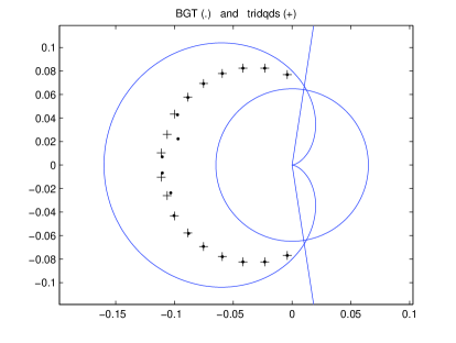
(a) $n=18$

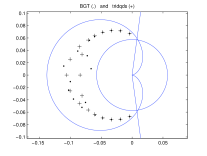
(b) $n=20$

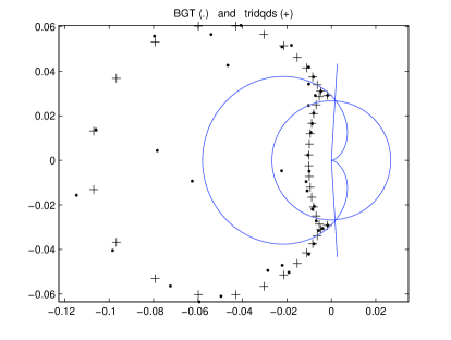
(c) $n=40$

Figure 3: Eigenvalues of Bessel matrix $B_{n}^{(-4.5,2)}$

Clement matrix

The so-called Clement matrices (see [3])

$$C=\operatorname{tridiag}(\boldsymbol{b},\boldsymbol{0},\boldsymbol{c})$$

with $b_{j}=j$ and $c_{j}=b_{n-j}$, $j=1,\ldots,n-1$, have real eigenvalues

$$\pm\;n-1,n-3,\ldots,1,\qquad\text{for }n\text{ even},$$

$$\pm\;n-1,n-3,\ldots,0,\qquad\text{for }n\text{ odd}.$$

These matrices posed no serious difficulties. The initial zero diagonal obliges the dqds based methods to take care when finding an initial $L,U$ factorization.

The tridqds code uses only real dqds transforms as it should. Our accuracy is less than $BGT$ but satisfactory. The complex dqds and tridqds performed identically. The ratio of elapsed times is the striking feature.

Our numerical tests have $n=100,200,400,800$. The minimum and maximum relative errors, $rel_{min}$ and $rel_{max}$, are shown in Table 2 and the CPU times in Table 3.

	$BGT$		complex dqds		tridqds
$n$	$rel_{min}$	$rel_{max}$	$rel_{min}$	$rel_{max}$	$rel_{mim}$	$rel_{max}$
100	$0$	$3\;10^{-16}$	$0$	$3\;10^{-14}$	$0$	$3\;10^{-14}$
200	$0$	$4\;10^{-16}$	$0$	$3\;10^{-13}$	$0$	$3\;10^{-13}$
400	$0$	$1\;10^{-15}$	$0$	$3\;10^{-12}$	$0$	$3\;10^{-12}$
800	$0$	$1\;10^{-15}$	$2\;10^{-16}$	$2\;10^{-12}$	$2\;10^{-16}$	$2\;10^{-12}$

Table 2: Relative errors for Clement matrices

$n$	$BGT$	complex dqds	tridqds
100	$4.2$	$0.06$	$0.06$
200	$12.6$	$0.12$	$0.13$
400	$42.2$	$0.45$	$0.50$
800	$174.2$	$1.8$	$1.8$

Table 3: CPU times in seconds for Clement matrices

Graded matrix

This matrix $C$ was created in $\Delta T$ form with $T=\operatorname{tridiag}(\boldsymbol{b},\boldsymbol{a},\boldsymbol{c})$,

$$a_{j} =b_{j}=c_{j}=3^{-(j-1)},\quad j=1,\ldots,n-1;\quad a_{n}=3^{-(n-1)},$$

and $\Delta=\mathop{\operator@font diag}\nolimits(\boldsymbol{\delta})$, $\delta_{j}=(-1)^{\lfloor(j+1)/2\rfloor}$, $j=1,\ldots,n$. The result is a balanced matrix with eigenvalues of different magnitude.

Figure 4 shows the approximated eigenvalues for $n=100$. Table 4 reports the CPU times.

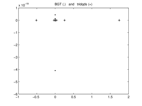
Figure 4: Eigenvalues of the graded matrix with $n=100$

$n$	$BGT$	complex dqds	tridqds
50	$0.31$	$0.02$	$0.02$
100	$0.67$	$0.06$	$0.04$
200	$2.12$	$0.14$	$0.06$
400	$...$	$0.45$	$0.35$

Table 4: CPU times in seconds for the graded matrices

$BGT$ code reported the message “Exceed maximum number of operations” for $n=400$. The performance of all methods for the flipped matrix is practically the same.

Matrix with clusters

Matrix Test 5 in [1],

$$C=D^{-1}\operatorname{tridiag}(\boldsymbol{1},\boldsymbol{\alpha},\boldsymbol{1}),\;\;D=\mathop{\operator@font diag}\nolimits(\boldsymbol{\beta}),\quad\boldsymbol{\alpha},\boldsymbol{\beta}\in\mathbb{R}^{n}\;\;\;$$

$$\alpha_{k}=10^{5(-1)^{k}}\cdot(-1)^{\lfloor k/4\rfloor},\;\;\beta_{k}=(-1)^{\lfloor k/3\rfloor},\quad k=1,\ldots,n,$$

seems to be a challenging test matrix. It was designed to have large, tight clusters of eigenvalues around $10^{-5}$, $-10^{5}$ and $10^{5}$. Half the spectrum is around $10^{-5}$ and the rest is divided unevenly between $-10^{5}$ and $10^{5}$. The diagonal alternates between entries of absolute value $10^{5}$ and $10^{-5}$ and so, for dqds codes, there is a lot of rearranging to do. When $n\geq 100$ it is not clear what is meant by accuracy.

All three codes obtain the correct number of eigenvalues in each cluster and the diameters of the clusters are all about $10^{-5}$. The striking feature is the time taken. See Table 5.

$n$	$BGT$	complex dqds	tridqds
50	$1.2$	$0.03$	$0.01$
100	$4.5$	$0.05$	$0.03$
200	$20.1$	$0.14$	$0.08$
400	$85.0$	$0.61$	$0.13$

Table 5: CPU times in seconds for Test 5 matrix

Matrix Test 4

For matrix Test 4 in [1],

$$C=D^{-1}\operatorname{tridiag}(\boldsymbol{1},\boldsymbol{\alpha},\boldsymbol{1}),\;\;D=\mathop{\operator@font diag}\nolimits(\boldsymbol{\beta}),\quad\boldsymbol{\alpha},\boldsymbol{\beta}\in\mathbb{R}^{n}\;\;\;$$

$$\alpha_{k}=(-1)^{k},\;\;\beta_{k}=20\cdot(-1)^{\lfloor k/5\rfloor},\quad k=1,\ldots,n,$$

the performance of the three codes is shown in Table 6. Figure 5 shows the eigenvalues of this matrix for $n=50$.

$n$	$BGT$	complex dqds	tridqds
50	$1.0$	$0.05$	$0.03$
100	$4.3$	$0.08$	$0.03$
200	$17.8$	$0.27$	$0.09$
400	$78.6$	$1.0$	$0.44$
800	$342.6$	$5.5$	$2.4$

Table 6: CPU times in seconds for Test 4 matrix

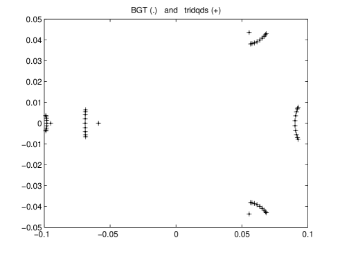
Figure 5: Eigenvalues of Test 4 matrix with $n=50$

Liu matrix

Z. A. Liu [13] devised an algorithm to obtain one-point spectrum unreduced tridiagonal matrices of arbitrary dimension $n\times n$. These matrices have only one eigenvalue, zero with multiplicity $n$, and the Jordan form consists of one Jordan block. Our code tridqds computes this eigenvalue exactly (and also the generalized eigenvectors) using the following method which is part of the prologue.

The best place to start looking for eigenvalues of a tridiagonal matrix $C=\operatorname{tridiag}(\boldsymbol{a},\boldsymbol{b},\boldsymbol{c})$ is at the arithmetic mean which we know $(\mu=\operatorname{trace}(C)/n)$. Before converting to $J-$form and factoring, we check whether $\mu$ is an eigenvalue by using the 3-term recurrence to solve

$$(\mu I-C)\boldsymbol{x}=\boldsymbol{e}_{n}p_{n}(\mu)/\prod_{i=1}^{n-1}c_{i}.$$

Here

$$x_{1} =1,\quad x_{2}=(\mu-a_{2})/c_{1},$$

$$x_{j+1} =\frac{1}{c_{j}}\left[(\mu-a_{j})x_{j}-b_{j-1}x_{j-1}\right],\quad j=2,\ldots,n-1,$$

and

$$\upsilon:=(\mu-a_{n})x_{n}-b_{n-1}x_{n-1}\left(=p_{n}(\mu)/\prod_{i=1}^{n-1}c_{i}\right).$$

If, by chance, $\upsilon$ vanishes, or is negligible compared to $\|\boldsymbol{x}\|$, then $\mu$ is an eigenvalue (to working accuracy) and $\boldsymbol{x}$ is an eigenvector. To check its multiplicity we differentiate with respect to $\mu$ and solve

$$(\mu I-C)\boldsymbol{y}=\boldsymbol{x}$$

with $y_{1}=0$, $y_{2}=1=x_{2}^{\prime}$ $(=x_{1})$. If

$$\upsilon^{\prime}=p_{n}^{\prime}(\mu)/\prod_{i=1}^{n-1}c_{i}:=(\mu-a_{n})y_{n}-b_{n-1}y_{n-1}+x_{n}$$

vanishes, or is negligible w.r.t. $\|\boldsymbol{y}\|$, then we continue the same way until the system is inconsistent or there are $n$ generalized eigenvectors.

Usually $\upsilon\neq 0$ and the calculation appears to have been a waste. This is not quite correct. In exact arithmetic, triangular factorization of $\mu I-C$ or $\mu I-J$, where $J=\Delta C\Delta^{-1}$, will break down if, and only if, $x_{j}$ vanishes for $1<j<n$. So our code examines $\min_{j}|x_{j}|$ and if it is too small w.r.t. its neighbors and w.r.t. $\|\boldsymbol{x}\|$ then we do not choose $\mu$ as our initial shift. Otherwise we do obtain initial $L$ and $U$ from $J-\mu I=LU$.

8 Conclusions and future work

We conclude that, working together, a single dqds transform with real shifts and our tridqds transform with complex conjugate pairs of shifts constitute the right tool for computing the eigenvalues of real tridiagonal matrices.

However there is far more work to be done for the following reasons. In a previous paper we discovered that, surprisingly often, eigenvalues are determined to, not high, but adequate relative accuracy; tiny relative changes $\eta$ in the parameters that define the matrix produce relative changes in the eigenvalue of the order of $10^{3}\eta$ or $10^{4}\eta$. This is good news. We cannot tell in advance when this occurs. In our opinion a relative condition number should be returned with each eigenvalue. This requires an approximation to the row and column eigenvectors, whether or not the user needs them.

We envision software that computes an initial approximation to each eigenvalue and then invokes a generalized Rayleigh quotient iteration to both compute eigenvectors and obtain a refined eigenvalue approximation, along with the smallest residual norms that could be achieved. Then the relative condition number can be formed. See [9].

Another practical feature is to scan the initial matrix to extract Gersgorin disks and a tight box in the complex plane that contains the spectrum. Matrices from industrial sources frequently permit “localization” of the eigenvectors belonging to certain parts of the spectrum. One consequence is that the relevant eigenvectors, and eigenvalues, may be obtained from small submatrices.

It is also important to scale and normalize the initial matrix and make use of the splitting that occurs with big matrices. Currently our shift strategy is quite straightforward and it is both difficult and worthwhile to improve it. There are plenty of challenges to be met before software for this real tridiagonal problem can be installed in packages such as LAPACK, not to mention parallel computation and scaLAPACK.

Appendix A Implementation details of minor step i

In this appendix we show how the calculations involved in each minor step of tridqds can be organized.

For each minor step $i,\;i=2,\ldots,n-3$, consider $F$ and $G$ as in (9). Denote the $2\times 1$ bulge in $F$, indicated with plus signs, by $\begin{bmatrix}x_{l}&y_{l}\end{bmatrix}^{T}$. And denote the entries $G_{i,i}$, $G_{i+1,i}$ and $G_{i+2,i}$, indicated with $*,+,+$, by $\begin{bmatrix}x_{r}&y_{r}&z_{r}\end{bmatrix}^{T}$. Subscripts $l$ and $r$ derive from “left” and “right”, respectively. This way we have

$$F=\begin{bmatrix}\ddots&&&&&\\ \ddots&1&&&&\\ &\hat{l}_{i-1}&u_{i}&1&&\\ &x_{l}&&u_{i+1}&1&\\ &y_{l}&&&u_{i+2}&\ddots\\ &&&&&\ddots\end{bmatrix},\qquad G=\begin{bmatrix}\ddots&\ddots&&&&\\ &\hat{u}_{i-1}&1&&&\\ &&x_{r}&&&\\ &&y_{r}&1&&\\ &&z_{r}&l_{i+1}&1&\\ &&&&\ddots&\ddots\end{bmatrix}$$

and the minor step $i$ can be accomplished using only these auxiliary variables.

$\underline{\textbf{Minor step {i}}}$

• • Matrices $Z_{i}^{-1}$ and $Z_{i}$

    $$Z_{i}^{-1}=\begin{bmatrix}\ddots&&&&&\\ &1&&&&\\ &&\frac{1}{u_{i}}&-\frac{1}{u_{i}}&&\\ &&0&1&&\\ &&&&1&\\ &&&&&\ddots\\ \end{bmatrix}, \qquad Z_{i}^{-1}=\begin{bmatrix}\ddots&&&&&\\ &1&&&&\\ &&u_{i}&1&&\\ &&0&1&&\\ &&&&1&\\ &&&&&\ddots\\ \end{bmatrix}$$

  • The effect of $Z_{i}^{-1}$ and the effect of $Z_{i}$

    $$FZ_{i}^{-1}=\begin{bmatrix}\ddots&&&&&\\ \ddots&1&&&&\\ &\hat{l}_{i-1}&1&0&&\\ &x_{l}&&u_{i+1}&1&\\ &y_{l}&&&u_{i+2}&\ddots\\ &&&&&\ddots\end{bmatrix}, \;Z_{i}G=\begin{bmatrix}\ddots&\ddots&&&&\\ &\hat{u}_{i-1}&1&&&\\ &&x_{r}&1&&\\ &&y_{r}&1&&\\ &&z_{r}&l_{i+1}&1&\\ &&&&\ddots&\ddots\end{bmatrix}$$

    where

    $$x_{r}\longleftarrow x_{r}*u_{i}+y_{r}\\$$

• • Matrices $\mathcal{L}_{i}^{-1}$ and $\mathcal{L}_{i}$

    $$\mathcal{L}_{i}^{-1}=\begin{bmatrix}\ddots&&&&&\\ &\ddots&&&&\\ &&1&&&\\ &&x_{l}&1&&\\ &&y_{l}&&1&\\ &&&&&\ddots\end{bmatrix},\qquad\mathcal{L}_{i}=\begin{bmatrix}\ddots&&&&&\\ &\ddots&&&&\\ &&1&&&\\ &&-x_{l}&1&&\\ &&-y_{l}&&1&\\ &&&&&\ddots\end{bmatrix}$$

    where

    $$\begin{array}[]{l}x_{l}\longleftarrow-x_{l}/\hat{l}_{i-1}\\ y_{l}\longleftarrow-y_{l}/\hat{l}_{i-1}\\ \end{array}$$

  • The effect of $\mathcal{L}_{i}^{-1}$

    $$\mathcal{L}_{i}^{-1}F=\begin{bmatrix}\ddots&&&&&\\ \ddots&1&&&&\\ &\hat{l}_{i-1}&1&&&\\ &&x_{l}&u_{i+1}&1&\\ &&y_{l}&&u_{i+2}&\ddots\\ &&&&&\ddots\end{bmatrix}$$

  • The effect of $\mathcal{L}_{i}$

    $$G\mathcal{L}_{i}=\begin{bmatrix}\ddots&\ddots&&&&\\ &\hat{u}_{i}&1&&\\ &x_{r}&1&&\\ &y_{r}&l_{i+1}&1&\\ &z_{r}&&l_{i+2}&1\\ &&&&\ddots&\ddots\end{bmatrix}$$

    where

    $$\begin{array}[]{l}\hat{u}_{i}\longleftarrow x_{r}-x_{l}\\ x_{r}\longleftarrow y_{r}-x_{l}\\ y_{r}\longleftarrow z_{r}-y_{l}-x_{l}*l_{i+1}\\ z_{r}\longleftarrow-y_{l}*l_{i+2}\\ \end{array}$$

• • Matrices $Y_{i}^{-1}$ and $Y_{i}$

    $$Y_{i}^{-1}=\begin{bmatrix}\ddots&&&&&\\ &1&&&\\ &x_{r}&1&&\\ &y_{r}&&1&\\ &z_{r}&&&1\\ &&&&&\ddots\end{bmatrix},\qquad Y_{i}=\begin{bmatrix}\ddots&&&&&\\ &1&&&\\ &-x_{r}&1&&\\ &-y_{r}&&1&\\ &-z_{r}&&&1\\ &&&&&\ddots\end{bmatrix}$$

    where

    $$\begin{array}[]{l}x_{r}\longleftarrow x_{r}/\hat{u}_{i}\\ y_{r}\longleftarrow y_{r}/\hat{u}_{i}\\ z_{r}\longleftarrow z_{r}/\hat{u}_{i}\\ \end{array}$$

  • The effect of $Y_{i}^{-1}$

    $$FY_{i}^{-1}=\begin{bmatrix}\ddots&&&&&\\ \ddots&1&&&&\\ &\hat{l}_{i}&u_{i+1}&1&&\\ &x_{l}&&u_{i+2}&1&\\ &y_{l}&&&u_{i+3}&\ddots\\ &&&&&\ddots\end{bmatrix}$$

    where

    $$\begin{array}[]{l}\hat{l}_{i}\longleftarrow x_{l}+y_{r}+x_{r}*u_{i+1}\\ x_{l}\longleftarrow y_{l}+z_{r}+y_{r}*u_{i+2}\\ y_{l}\longleftarrow z_{r}*u_{i+3}\\ \end{array}$$

  • The effect of $Y_{i}$

    $$Y_{i}G=\begin{bmatrix}\ddots&\ddots&&&&\\ &\hat{u}_{i}&1&&&\\ &&x_{r}&&&\\ &&y_{r}&1&&\\ &&z_{r}&l_{i+2}&1&\\ &&&&\ddots&\ddots\end{bmatrix}$$

    where

    $$\begin{array}[]{l}x_{r}\longleftarrow 1-x_{r}\\ y_{r}\longleftarrow l_{i+1}-y_{r}\\ z_{r}\longleftarrow-z_{r}\\ \end{array}$$

Appendix B tridqds algorithm

$$\begin{array}[]{rll}\textsl{tridqds}(\sigma,\bar{\sigma}):&\\ \\ &\textsf{\% \text{ step } 1}\\ &x_{r}=1;\;\;y_{r}=l_{1};\;\;z_{r}=0\\ &\textsf{\% \text{ the effect of $Z_{1}$}}\\ &x_{r}=x_{r}*u_{1}+y_{r}\\ &\textsf{\% \text{ the matrix $\mathcal{L}_{1}^{-1}$}}\\ &x_{l}=(u_{1}+l_{1})^{2}+u_{2}l_{1}-2(\Re\sigma)(u_{1}+l_{1})+|\sigma|^{2}\\ &y_{l}=-u_{2}l_{1}u_{3}l_{2}/x_{l}\\ &x_{l}=-u_{2}l_{1}(u_{1}+l_{1}+u_{2}+l_{2}-2(\Re\sigma))/x_{l}\\ &\textsf{\% \text{ the effect of $\mathcal{L}_{1}$}}\\ &\hat{u}_{1}=x_{r}-x_{l};\\ &x_{r}=y_{r}-x_{l};\;\;y_{r}=z_{r}-y_{l}-x_{l}*l_{2};\;\;z_{r}=-y_{l}*l_{3}\\ &\textsf{\% \text{ the matrix $Y_{1}^{-1}$}}\\ &x_{r}=x_{r}/\hat{u}_{1};\;\;y_{r}=y_{r}/\hat{u}_{1};\;\;z_{r}=z_{r}/\hat{u}_{1}\\ &\textsf{\% \text{ the effect of $Y_{1}^{-1}$}}\\ &\hat{l}_{1}=x_{l}+y_{r}+x_{r}*u_{2}\\ &x_{l}=y_{l}+z_{r}+y_{r}*u_{3};\;\;y_{l}=z_{r}*u_{4}\\ &\textsf{\% \text{ the effect of $Y_{1}$}}\\ &x_{r}=1-x_{r};\;\;y_{r}=l_{2}-y_{r};\;\;z_{r}=-z_{r}\\ \\ \end{array}$$

$$\begin{array}[]{rll}&\\ &\textbf{for }i=2,\ldots,n-3\\ &\hskip 17.07182pt\textsf{\% \text{ the effect of $Z_{i}$}}\\ &\hskip 17.07182ptx_{r}=x_{r}*u_{i}+y_{r}\\ &\hskip 17.07182pt\textsf{\% \text{ the matrix $\mathcal{L}_{i}^{-1}$}}\\ &\hskip 17.07182ptx_{l}=-x_{l}/\hat{l}_{i-1};\;\;y_{l}=-y_{l}/\hat{l}_{i-1};\\ &\hskip 17.07182pt\textsf{\% \text{ the effect of $\mathcal{L}_{i}$}}\\ &\hskip 17.07182pt\hat{u}_{i}=x_{r}-x_{l};\\ &\hskip 17.07182ptx_{r}=y_{r}-x_{l};\;\;y_{r}=z_{r}-y_{l}-x_{l}*l_{i+1};\;\;z_{r}=-y_{l}*l_{i+2}\\ &\hskip 17.07182pt\textsf{\% \text{ the matrix $Y_{i}^{-1}$}}\\ &\hskip 17.07182ptx_{r}=x_{r}/\hat{u}_{i};\;\;y_{r}=y_{r}/\hat{u}_{i};\;\;z_{r}=z_{r}/\hat{u}_{i}\\ &\hskip 17.07182pt\textsf{\% \text{ the effect of $Y_{i}^{-1}$}}\\ &\hskip 17.07182pt\hat{l}_{i}=x_{l}+y_{r}+x_{r}*u_{i+1}\\ &\hskip 17.07182ptx_{l}=y_{l}+z_{r}+y_{r}*u_{i+2};\;\;y_{l}=z_{r}*u_{i+3}\\ &\hskip 17.07182pt\textsf{\% \text{ the effect of $Y_{i}$}}\\ &\hskip 17.07182ptx_{r}=1-x_{r};\;\;y_{r}=l_{i+1}-y_{r};\;\;z_{r}=-z_{r}\\ &\textbf{end for}\\ \\ \end{array}$$

$$\begin{array}[]{rll}&\\ &\textsf{\% \text{ step } n-2}\\ &\textsf{\% \text{ the effect of $Z_{n-2}$}}\\ &x_{r}=x_{r}*u_{n-2}+y_{r}\\ &\textsf{\% \text{ the matrix $\mathcal{L}_{n-2}^{-1}$}}\\ &x_{l}=-x_{l}/\hat{l}_{n-3};\;\;y_{l}=-y_{l}/\hat{l}_{n-3};\\ &\textsf{\% \text{ the effect of $\mathcal{L}_{n-2}$}}\\ &\hat{u}_{n-2}=x_{r}-x_{l};\\ &x_{r}=y_{r}-x_{l};\;\;y_{r}=z_{r}-y_{l}-x_{l}*l_{n-1}\\ &\textsf{\% \text{ the matrix $Y_{n-2}^{-1}$}}\\ &x_{r}=x_{r}/\hat{u}_{n-2};\;\;y_{r}=y_{r}/\hat{u}_{n-2}\\ &\textsf{\% \text{ the effect of $Y_{n-2}^{-1}$}}\\ &\hat{l}_{n-2}=x_{l}+y_{r}+x_{r}*u_{n-1}\\ &x_{l}=y_{l}+y_{r}*u_{n}\\ &\textsf{\% \text{ the effect of $Y_{n-2}$}}\\ &x_{r}=1-x_{r};\;\;y_{r}=l_{n-1}-y_{r}\\ \\ \end{array}$$

$$\begin{array}[]{rll}&\textsf{\%\text{ step } n-1 }\\ &\textsf{\% \text{ the effect of $Z_{n-1}$}}\\ &x_{r}=x_{r}*u_{n-1}+y_{r}\\ &\textsf{\% \text{ the matrix $\mathcal{L}_{n-1}^{-1}$}}\\ &x_{l}=-x_{l}/\hat{l}_{n-2}\\ &\textsf{\% \text{ the effect of $\mathcal{L}_{n-1}$}}\\ &\hat{u}_{n-1}=x_{r}-x_{l};\\ &x_{r}=y_{r}-x_{l}\\ &\textsf{\% \text{ the matrix $Y_{n-1}^{-1}$}}\\ &x_{r}=x_{r}/\hat{u}_{n-1}\\ &\textsf{\% \text{ the effect of $Y_{n-1}^{-1}$}}\\ &\hat{l}_{n-1}=x_{l}+x_{r}*u_{n}\\ &\textsf{\% \text{ the effect of $Y_{n-1}$}}\\ &x_{r}=1-x_{r}\\ \\ \end{array}$$

$$\begin{array}[]{rll}&\textsf{{\%\text{ step } n}}\\ &\%\textsf{ the effect of $Z_{n}$}\\ &x_{r}=x_{r}*u_{n}\\ &\textsf{\% \text{ the matrix $\mathcal{L}_{n}^{-1}=I$}}\\ &\textsf{\% \text{ the effect of $\mathcal{L}_{n}$}}\\ &\hat{u}_{n}=x_{r};\\ &\textsf{\% \text{ the matrix $Y_{n}^{-1}=I$}}\\ \end{array}$$

References

- [1] D. A. Bini, L. Gemignani and F. Tisseur. The Ehrlich-Aberth method for the nonsymmetric tridiagonal eigenvalue problem. SIAM J. Matrix Analysis and its Aplications, 27(1):153-175, 2005.
- [2] A. Bunse-Gerstner. An analysis of the HR algorithm for computing the eigenvalues of a matrix. Linear Algebra and Its Applications, 35:155-173, 1981.
- [3] P. A. Clement. A class of triple-diagonal matrices for test purposes. SIAM Review, 1 (vol.1), January, 1959.
- [4] Jane K. Cullum.A QL procedure for computing the eigenvalues of complex symmetric tridiagonal matrices. SIAM J. Matrix Analysis and its Aplications, 17(1):83-109, 1996.
- [5] D. Day. Semi-duality in the two-sided lanczos algorithm. Ph.D thesis, University of California, Berkeley, 1993.
- [6] I. S. Dhillon and B. N. Parlett. Multiple representations to compute orthogonal egenvectors of symmetric tridiagonal matrices. Linear Algebra and its Applications, 387:1-28, 2004.
- [7] K. Fernando and B. Parlett.Accurate singular values and differential qd algorithms. Numerische Mathematik, 67:191-229, 1994.
- [8] C. Ferreira. The unsymmetric tridiagonal eigenvalue problem. Ph.D Thesis, University of Minho, 2007. http://hdl.handle.net/1822/6761
- [9] C. Ferreira and B. Parlett. Sensitivity of Eigenvalues of an unsymmetric tridiagonal matrix. Submitted.
- [10] C. Ferreira and B. Parlett. Convergence of LR algorithm for a one-point spectrum tridiagonal matrix. Numerische Mathematik, 113(3):417-431, 2009.
- [11] C. Ferreira and B. Parlett. Sensitivity of Eigenvalues of an unsymmetric tridiagonal matrix. Submitted.
- [12] J. G. F. Francis. The QR transformation - a unitary analogue to the LR transformation, Parts I and II. Computer Journal, 4:265-272 and 332-245, 1961/62.
- [13] Z. A. Liu. On the extended HR algorithm. Technical Report PAM-564, Center for Pure and Applied Mathematics, University of California, Berkeley, CA, USA, 1992.
- [14] B. N. Parlett. Reduction to tridiagonal form and minimal realizations, SIAM Jornal on Matrix Analysis, 13:567-593, 1992.
- [15] B. N. Parlett. The new qd algorithms. Acta Numerica, 459-491, 1995.
- [16] B. N. Parlett and Osni A. Marques. An implementation of the dqds algorithm. Linear Algebra and Its Applications, 309:217-259, 2000.
- [17] L. Pasquini. Accurate computation of the zeros of the generalized Bessel polynomials. Numerische Mathematic, 86:507-538, 2000.
- [18] H. Rutishauser. Solution of eigenvalue problems with the LR-transformation. National Bureau of Standards Applied Mathematics series 49:47-81, 1958.
- [19] H. Rutishauser and H.R. Schwarz. The LR transformation method for symmetric matrices. Numerische Mathematik, 5:273-289, 1963.
- [20] J. Slemons. The Result of Two Steps of the LR Algorithm is Diagonally Similar to the Result of One Step of the HR Algorithm . SIAM J. Matrix Analysis and its Aplications, 31(1):68-74, 2009.
- [21] D. S. Watkins. QR-like algorithms - An overview of convergence theory and practice. Lectures in Applied Mathematics, 32:879-893, 1996.
- [22] D. S. Watkins and L. Elsner. Convergence of algorithms of decomposition type for the eigenvalue problem. Linear Algebra and Its Applications, 143:19-47, 1991.
- [23] Z. Wu. The Triple dqds Algorithm for Complex Eigenvalues. Ph.D thesis, University of California, Berkeley, 1996.
- [24] H. Xu. The relation between the QR and LR algorithms. SIAM J. Matrix Analysis and its Aplications, 19(2):551-555, 1998.
- [25] Yao Yang. Error Analysis of the qds and dqds Algorithms. Ph.D thesis, University of California, Berkeley, 1994.