Model selection for spectro-polarimetric inversions

Abstract

Inferring magnetic and thermodynamic information from spectropolarimetric observations relies on the assumption of a parameterized model atmosphere whose parameters are tuned by comparison with observations. Often, the choice of the underlying atmospheric model is based on subjective reasons. In other cases, complex models are chosen based on objective reasons (for instance, the necessity to explain asymmetries in the Stokes profiles) but it is not clear what degree of complexity is needed. The lack of an objective way of comparing models has, sometimes, led to opposing views of the solar magnetism because the inferred physical scenarios are essentially different. We present the first quantitative model comparison based on the computation of the Bayesian evidence ratios for spectropolarimetric observations. Our results show that there is not a single model appropriate for all profiles simultaneously. Data with moderate signal-to-noise ratios favor models without gradients along the line-of-sight. If the observations shows clear circular and linear polarization signals above the noise level, models with gradients along the line are preferred. As a general rule, observations with large signal-to-noise ratios favor more complex models. We demonstrate that the evidence ratios correlate well with simple proxies. Therefore, we propose to calculate these proxies when carrying out standard least-squares inversions to allow for model comparison in the future.

1. Introduction

Spectropolarimetry is a very powerful diagnostic technique. It has allowed us to study in depth the thermodynamical and magnetic properties of the solar and stellar plasmas. However, the valuable information encoded in the Stokes profiles is often difficult to extract. The response of the spectral shape of a given spectral line to changes of the properties of the plasma is very convoluted, non-linear and, in many occasions, non-local.

In spite of the complex relation between the physical parameters and the emergent Stokes profiles, several simple diagnostic tools have been developed in the past and are still under wide use in solar physics. Among them, the line ratio technique (Stenflo, 1973, 2010, 2011), the center-of-gravity method (Semel, 1970; Rees & Semel, 1979) and the application of calibration curves between spectral line and magnetic field properties (e.g., Lites et al., 2008; Martínez Pillet et al., 2011, for recent applications) have had special relevance.

During the last few decades we have witnessed the development and systematic application of nonlinear inversion codes. They extract physically relevant information by comparing the observed Stokes profiles to those synthesized in appropriate atmospheric models. Because of the non-linearity between the physical parameters and the observables, these inversion methods make use of elaborate time-consuming non-linear optimization methods. The first heroic (because of the low computational power available at that time) efforts made use of relatively simple physical models, of which the Milne-Eddington (ME) approximation is the most widely spread (e.g., Harvey et al., 1972; Auer et al., 1977; Landi Degl’Innocenti & Landolfi, 2004). Although the simplifying assumptions made by the ME approximation may not be fully fulfilled in real solar plasmas, it is still one of the most widely used models, in part, because of its analytical simplicity. Even state-of-the-art inversion codes such as VFISV (Borrero et al., 2007, 2010), used for inferring magnetic field vectors from the Helioseismic and Magnetic Imager (HMI; onboard the Solar Dynamics Observatory) data, or as MILOS (Orozco Suárez et al., 2007) and MERLIN (Skumanich & Lites, 1987; Lites et al., 2007), currently applied to data from the Hinode spacecraft, are based on this assumption.

The increase in computational power made it feasible to use more elaborate models. A fundamental leap forward was the application of the idea of response functions (Landi Degl’Innocenti & Landi Degl’Innocenti, 1977) to the inversion of Stokes profiles with non-trivial depth stratifications of the physical quantities. The first representative of this family of codes was SIR (Stokes Inversion based on Response functions; Ruiz Cobo & del Toro Iniesta, 1992). The presence of gradients along the line-of-sight (LOS) of the physical properties are of importance for explaining the strong asymmetries observed in magnetized regions (Solanki & Pahlke, 1988; Grossmann-Doerth et al., 1988; Solanki & Montavon, 1993; Sigwarth et al., 1999; Khomenko et al., 2003; Martínez González et al., 2008; Viticchié & Sánchez Almeida, 2011). Based on the same strategy, Socas-Navarro et al. (1998) developed a code capable of dealing with lines in NLTE (non-local thermodynamical equilibrium). This model has been mainly applied for the inversion of Ca ii infrared triplet lines, which are formed under strong NLTE conditions (e.g., Socas-Navarro et al., 2000; de la Cruz Rodríguez et al., 2010).

Models based on the assumption of microstructured magnetic atmospheres which incorporate small-scale fluctuations of the physical quantities along the LOS have also been proposed (Sánchez Almeida, 1997). A property of such models is the natural generation of asymmetric profiles, which has been proposed as an alternative to explain the observed asymmetries (Sánchez Almeida et al., 1989; Sánchez Almeida & Lites, 2000; Viticchié et al., 2011).

The history of inversion codes displays an interesting characteristic. The complexity of the models proposed has increased with time thanks to two factors. First, the computational power has allowed us to solve the non-linear optimization problem faster. Second, the quality of spectropolarimetric observations has improved with time, with instruments systematically achieving signal-to-noise ratios above 1000 and reaching 10⁴ in many cases. This forces the inversion code to fit minute variations of the shape of the Stokes profile. In many cases, such small modifications of the shape of the profiles are encoding important physical effects.

Although counterintuitive, the availability of high-quality observations has also intensified a discussion that has been present from the beginning of the history of inversion codes. The selection of the model to be used for the inversions is often influenced by subjective reasons. A model can be chosen deliberately to be simple because of the necessity of inverting large maps as fast as possible. This is the case of HMI (Borrero et al., 2010). An inversion code based on a given model is sometimes chosen based on the availability of the inversion code and the expertise to use it. A model might be chosen based on its capability to fit as much detail of the Stokes profiles as possible. Sometimes the selection of a model is driven by spatial resolution. This is the case when there is a clear indication in the spectrum that structures are not resolved. Other possibilities can be invoked, but they sometimes contain a large subjective content.

The choice of the model is also important because it critically affects the interpretation of the inferred parameters. This is specially relevant for parameters that are more indirectly related to observables, like the magnetic field of non-resolved structures. There are widespread examples in the literature, especially when signals are weak. For instance, there has been some controversy regarding the magnetic field strength in the quiet Sun inferred from infrared or visible Fe i lines (e.g., Khomenko et al., 2003; Lites & Socas-Navarro, 2004; Domínguez Cerdeña et al., 2006; Martínez González et al., 2008). More recently, conflicting properties of the magnetic field in internetwork regions of the quiet Sun have been obtained by Lites et al. (2008) and Orozco Suárez et al. (2007) on the one hand, and by Stenflo (2010) on the other, from the very same Hinode observations (and partially supported with data from ground by Beck & Rezaei, 2009). These discrepancies are only “apparent” because they are caused by the application of different modelings when the organization of internetwork magnetic fields is still an unknown. Once we know the nature of the magnetic fields in the quiet Sun or, in other words, we have access to the most probable model among all possible ones, the results will be reliable. This problem does not arise for parameters that are more directly related to observables like bulk velocities, field azimuths, magnetic flux, etc.

This paper does not deal with the actual implementation of particular inversion algorithms and codes, or their respective efficiencies, but with the suitability of the underlying physical models to explain the observations. To this aim we perform the first fully Bayesian comparison of models for the inversion of Stokes profiles. To this end, we analyze a sample of Stokes profiles observed with the spectropolarimeter (SP; Lites et al., 2001) aboard Hinode (Kosugi et al., 2007) and with the vector magnetograph IMaX (Martínez Pillet et al., 2011) onboard the Sunrise balloon (Solanki et al., 2010). We discuss, for different cases, the model (chosen from a pool of fixed models) that is favored by data and their relative probabilities based on the computation of the evidence. The evidence is calculated using the Bayesian inference code developed by Asensio Ramos et al. (2007) and recent extensions that we have made to the code to deal with models with gradient.

2. Model selection theory

We apply model selection theory to determine which is the model best suited for explaining the Stokes profiles observed in a pixel (e.g., Trotta, 2008, for a general description and more details). Let’s assume we have $N_{\mathrm{mod}}$ models $\{\mathcal{M}_{i},i=1\ldots N_{\mathrm{mod}}\}$ competing to explain the same set of observations formally represented by $D$. Here, $D$ will be represented by a formal vector $\mathbf{d}=[I(\lambda_{1}),I(\lambda_{2}),...,Q(\lambda_{1}),...,U(\lambda_{1}),...,V(\lambda_{1}),...]$ whose elements are the values of the Stokes parameters $I$, $Q$, $U$, and/or $V$ at certain wavelengths $\lambda_{1},\lambda_{2},...$. By a model we mean an algorithm that depends on a set of $N_{j}^{(i)}$ parameters $\mbox{\boldmath$\theta$}_{i}=(\theta_{i;1},\theta_{i;2},...,\theta_{i;N_{j}^{(i)}})$ (often, the temperature at one or several points in a model atmosphere; the magnetic field strength, in clination, and azimuth; the density, etc), whose output is a prediction $\mathbf{y}(\mbox{\boldmath$\theta$}_{i})$ of the data. The Bayes theorem (Jaynes, 2003; MacKay, 2003; Gregory, 2005) states that the posterior probability of each model at the light of the obs erved data is

$$p(\mathcal{M}_{i}|D)=\frac{p(D|\mathcal{M}_{i})p(\mathcal{M}_{i})}{p(D)},$$ (1)

where $p(\mathcal{M}_{i})$ is our prior belief in each model (which we will assume to be the same for all the models considered here; see below), while $p(D)$ is just a normalization constant:

$$p(D)=\sum_{i=1}^{N_{\mathrm{mod}}}p(D|\mathcal{M}_{i})p(\mathcal{M}_{i}).$$ (2)

Finally, $p(D|{\cal M}_{i})$ is the evidence or marginal likelihood, which is the key ingredient of our model comparison, and is given by the following integral (e.g., Trotta, 2008; Asensio Ramos, 2011):

$$p(D|\mathcal{M}_{i})=\int\mathrm{d}\mbox{\boldmath$\theta$}_{i}p(\mbox{\boldmath$\theta$}_{i}|\mathcal{M}_{i})p(D|\mbox{\boldmath$\theta$}_{i},\mathcal{M}_{i}).$$ (3)

The quantity $p(\mbox{\boldmath$\theta$}_{i}|\mathcal{M}_{i})$ is the prior distribution for the model parameters. If, for example, we assume that $\theta_{i;j}$ (i.e., the $j$-th parameter of mode $i$) is a priori distributed uniformly between $\theta_{i;j}^{\mathrm{min}}$ and $\theta_{i;j}^{\mathrm{max}}$, then

$$p(\theta_{i}^{j}|\mathcal{M}_{i})=\left\{\begin{array}[]{clc}\left[\theta_{i;j}^{\mathrm{max}}-\theta_{i;j}^{\mathrm{min}}\right]^{-1}&&\theta_{i;j}^{\mathrm{min}}<\theta_{i;j}<\theta_{i;j}^{\mathrm{max}}\\ 0&&\mathrm{otherwise}\end{array}\right..$$ (4)

The quantity $p(D|\mbox{\boldmath$\theta$}_{i},\mathcal{M}_{i})$ in Eq. (3) is the likelihood, which is computed from the observed data. Assuming that the observations are corrupted with uncorrelated Gaussian random noise, then

$$p(D|\mbox{\boldmath$\theta$}_{i},\mathcal{M}_{i})=\prod_{j=1}^{M}\left(2\pi\sigma_{j}^{2}\right)^{-1/2}\exp\left[-\frac{\left(y_{j}(\mbox{\boldmath$\theta$}_{i})-d_{j}\right)^{2}}{2\sigma_{j}^{2}}\right],$$ (5)

(for mode details, see Asensio Ramos et al., 2007; Asensio Ramos, 2009). In general, we will assume our priors to be uniform (Eq. 4), hence, the evidence in Eq. (3) simply reads:

$$p(D|\mathcal{M}_{i})=\left[\prod_{j=1}^{N_{i}}\frac{1}{(\theta_{i}^{j})^{\mathrm{max}}-(\theta_{i}^{j})^{\mathrm{min}}}\right]\int_{\Omega}\mathrm{d}\mbox{\boldmath$\theta$}_{i}p(D|\mbox{\boldmath$\theta$}_{i},\mathcal{M}_{i}),$$ (6)

where the integral is computed extended over the volume $\Omega$ which contains the region where the priors are non-zero. It is important to note that, if a model parameter is completely unconstrained by the observed data (so the ensuing likelihood does not depend on this parameter), the evidence does not penalize it because it factorizes from the integral.

Given two models, $\mathcal{M}_{0}$ and $\mathcal{M}_{1}$ that are proposed to explain an observation, the ratio of posteriors

$$\frac{p(\mathcal{M}_{0}|D)}{p(\mathcal{M}_{1}|D)}=\frac{p(\mathcal{M}_{0})}{p(\mathcal{M}_{1})}\frac{p(D|\mathcal{M}_{0})}{p(D|\mathcal{M}_{1})},$$ (7)

is used to compute how more probable one model is with respect to the other (Jeffreys, 1961). The ratio of evidences is known as the Bayes factor, $B_{01}$, and it is trivially given by:

$$B_{01}=\frac{p(D|\mathcal{M}_{0})}{p(D|\mathcal{M}_{1})}.$$ (8)

If both models are assumed to have the same a-priori probability (which is what we have assumed in all subsequent computations), the ratio of posteriors is just the Bayes factor. Large values of $B_{01}$ indicate a preference for model $\mathcal{M}_{0}$ while small values indicate a preference for model $\mathcal{M}_{1}$. Table 2 gives the modified Jeffreys scale that can be used to translate values of the Bayes factor into strengths of belief (Jeffreys, 1961; Kass & Raftery, 1995; Gordon & Trotta, 2007).

Table 1Modified empirical Jeffreys’ scale (taken from Trotta, 2008)

$|\ln B_{01}|$	Odds	Strength of evidence
$<1.0$	$\lesssim 3:1$	Inconclusive
$1.0$	$\sim 3:1$	Weak evidence
$2.5$	$\sim 12:1$	Moderate evidence
$5.0$	$\sim 150:1$	Strong evidence

Therefore, model comparison is a matter of computing $p(\mathcal{M}_{i}|D)$ for all models and calculating their ratios for pairs of models. As shown by Eq. (3), the evidence contains a balance between the quality of the fit (encoded in the likelihood) and the number of parameters (encoded on the prior). In order to gain some insight consider the following example. Let ${\cal M}_{1}$ be a model with a single parameter $\theta$, and ${\cal M}_{0}$ another one with this parameter fixed to the value $\theta_{0}$. If the prior on the parameter for ${\cal M}_{1}$ is flat with a range $\Delta\theta$ sufficiently large to acommodate the likelihood, then

$$p(\theta|\mathcal{M}_{0}) = \delta(\theta-\theta_{0})$$

$$p(\theta|\mathcal{M}_{1}) = \left\{\begin{array}[]{clc}\frac{1}{\Delta\theta}&&\theta_{i;j}^{\mathrm{min}}<\theta_{i;j}<\theta_{i;j}^{\mathrm{max}}\\ 0&&\mathrm{otherwise}\end{array}\right.$$ (11)

Now, let the likelihood be a relatively peaked function around the value $\bar{\theta}$, with a characteristic width $\delta\theta$, then, from Eq. (3) the evidences in both cases read

$$p(D|\mathcal{M}_{0}) = p(D|\theta_{0},\mathcal{M}_{1})$$

$$p(D|\mathcal{M}_{1}) \approx p(D|\hat{\theta},\mathcal{M}_{1})\frac{\delta\theta}{\Delta\theta},$$ (12)

Assuming identical priors for both models, the evidence ratio is

$$\frac{p(D|\mathcal{M}_{1})}{p(D|\mathcal{M}_{0})}\approx\frac{p(D|\hat{\theta},\mathcal{M}_{1})}{p(D|\theta_{0},\mathcal{M}_{0})}\frac{\delta\theta}{\Delta\theta}.$$ (13)

Consequently, since the ratio of likelihoods has to be larger than or equal to 1 (model $\mathcal{M}_{1}$ contains model $\mathcal{M}_{0}$), model $\mathcal{M}_{1}$ is preferred to model $\mathcal{M}_{0}$ when the prior space is not so large with respect to the width of the likelihood. This shows that the evidence ratio works as a Bayesian Occam’s razor.

The main difficulty in model comparison is that the evidence in Eq. (3) is computationally very demanding because it is the result of a high-dimensional integral (e.g., Trotta, 2008, and references therein). In recent years, some efficient algorithms, specially those based on nested sampling (Skilling, 2004), have been developed to deal with this problem. The codes that we use in this paper make use of the Multinest algorithm (Feroz et al., 2009) which performs very well in our cases.

3. Observations

3.1. Spectropolarimetry

We select the profiles for the application of the Bayesian model comparison for spectropolarimetric data from a representative sample of what one can find in the solar photosphere. For the quiet Sun, they have been extracted from the observations analyzed by Lites et al. (2008). They were obtained at disk center on 2007 March 10 with the spectropolarimeter SOT/SP aboard Hinode with a spatial resolution of $\sim 0.32^{\prime\prime}$. The observed spectral region consists of the Fe i doublet at 6301.5 and 6302.5 Å with a spectral resolution close to 3$\times$10⁵, resulting in a total of 112 wavelength points. After calibration, the standard deviation of the noise in Stokes $Q$, $U$ and $V$ in units of the continuum is estimated to be of the order of 1.1-1.2$\times$10^-3. Likewise, the standard deviation of Stokes $I$ computed on a continuum window is estimated to be $\sim$6$\times$10^-3, the increase being probably produced by flat-fielding effects. Given the large computational effort that the estimation of the evidence requires, we have focused on individual profiles extracted from the Stokes $V$ classification calculated by Viticchié et al. (2011) using a k-means unsupervised classification algorithm widely used in machine learning (Everitt, 1995; Bishop, 2006). We have selected individual profiles from the observations whose polarization amplitude is, in any of the Stokes parameters, above a threshold of 4.5 times the standard deviation of the noise. This way, we avoid large uncertainties in the model parameters as pointed out by Asensio Ramos (2009). The considered profiles are shown in black curves in Fig. 1 and their classification, including the nomenclature for the shape of the profiles used by Viticchié et al. (2011) is displayed in Table 4. Of the six groups available (network, blue-lobe, red-lobe, asymmetric, antisymmetric and $Q$-like), we have picked representative profiles, some of them having no apparent linear polarization above the noise threshold and some of them showing clear signals. We consider that they represent a good sample of what one can find in the quiet Sun observed with Hinode.

Concerning the profiles associated to umbra and penumbra, they were extracted from Hinode observations obtained on 2007 February 27. The estimated noise level in the umbra for Stokes $Q$, $U$ and $V$ is of the order of 5$\times$10^-3 in units of the continuum intensity, while it increases to 0.02 for Stokes $I$. The noise level is much larger than for the quiet Sun profiles, partly because of the reduced number of photons and also because of the apperance of molecular lines that we do not fit.

3.2. Imaging polarimetry

Four IMaX observations have been chosen to study model comparison in imaging polarimetric data. The first one is characterized by Stokes $V$ above the noise level and Stokes $Q$ and $U$ below the noise. The second one has Stokes $Q$ and $U$ above the noise and $V$ below. The third has all Stokes parameters above the noise, while the fourth has all Stokes parameters below the noise. The analysis of model comparison for the inversion of these profiles is of special relevance given their low spectral sampling. The observations consist of the four Stokes parameters at $-80$, $-40$, $+40$, $+80$ and $+227$ mÅ around the Fe i line at 5250.209 Å. The spectral point spread function (PSF) has very extended tails, typical of Fabry-Pérot instruments. Instead of taking it into account exactly, we follow Lagg et al. (2010) who substituted the real PSF by a Gaussian PSF of 85 mÅ ($\sim 2.9$ km s^-1) of full width at half-maximum (FWHM). Although the Gaussian PSF does not present extended tails, its convolution with the FTS spectrum gives line profiles similar to those obtained using the correct PSF (see Martínez Pillet et al., 2011).

The estimated noise level is 4$\times$10^-3 for Stokes $I$ and 10^-3 for Stokes $Q$, $U$ and $V$, all in units of the continuum intensity. The spatial resolution of the instrument is estimated to be between 0.15^′′ and 0.18^′′ (Lagg et al., 2010).

Table 6 shows some interesting properties of the observed Stokes profiles: $P_{\mathrm{tot}}$ is the maximum total polarization, $P_{V}$ is the maximum circular polarization, $a$ and $A$ are the area and amplitude asymmetries respectively (e.g., Solanki & Stenflo, 1986), while $v_{\mathrm{V}}$ and $v_{\mathrm{I}}$ are the Stokes $V$ zero-crossing velocity and the Stokes $I$ velocity of the minimum. The velocities are related to the rest wavelength of the spectral lines (they are not absolute). The sign of the area asymmetry is chosen equal to the sign of the bluest peak of Stokes $V$, following Martínez Pillet et al. (1997). We have not tabulated the asymmetries for the IMaX data because we are not confident on their values with only 5 points in wavelength and of class 34 because it clearly shows the presence of several lobes making the definition of asymmetries invalid.

4. Atmospheric models

Among the infinitely many models one might build to reproduce the emergent Stokes profiles from a magnetized atmosphere, we consider for our analysis those most widely used in the literature. All of them are based on different approximations for the solution of the radiative transfer equation for polarized radiation in a plane-parallel atmosphere (see Landi Degl’Innocenti & Landolfi, 2004):

$$\frac{d\mathbf{S}}{dz}=\mbox{\boldmath$\epsilon$}-\mathbf{K}\mathbf{S},$$ (14)

where $z$ is the spatial coordinate along the ray, $\mathbf{S}=(I,Q,U,V)^{t}$ is the Stokes vector, $\epsilon$ the emissivity vector, and $\mathbf{K}$ the propagation matrix.

All models considered assume local thermodynamic equilibrium. Therefore, $\epsilon$ and $\mathbf{K}$ depend on the local thermodynamic and magnetic properties of the medium but not on $\mathbf{S}$ itself. Three types of hypotheses are assumed for the variation of $\epsilon$ and $\mathbf{K}$ with $z$: i) constant along the line of sight, ii) some thermodynamic quantities vary (linearly) but the magnetic field is constant, iii) all quantities may vary with $z$. Finally, we consider models with a single atmosphere occupying the whole element, and models with two independent atmospheres within the same resolution element. In the latter case, the emergent Stokes profiles are given by

$$\mathbf{S}=f\mathbf{S}_{1}+(1-f)\mathbf{S}_{2},$$ (15)

where $\mathbf{S}_{1}$ and $\mathbf{S}_{2}$ are the emergent profiles of each of the two components, which occupy fractions $f$ and $(1-f)$ of the pixel, respectively. Two possibilities are considered for these two components. First, $\mathbf{S}_{1}$ corresponds to a magnetic component (hence, $Q,U$, and $V$ are, in general, non-zero), while $\mathbf{S}_{2}$ forms in a field-free atmosphere (hence, $Q=U=V=0$). Second, both atmospheres are magnetized.

In these models, we consider the formation of the widely used Fe i 630 nm doublet and the 5250.2 Å line. The atomic data for the synthesis of the lines has been compiled from the VALD database (Piskunov et al., 1995; Kupka et al., 1999). The data is summarized in Table 2. Collisional broadening is treated under the formalism of Anstee & O’Mara (1995) for the broadening of spectral lines (only for allowed transitions), with the velocity parameter ($\alpha$) and the line broadening cross section ($\sigma$, in units of $a_{0}^{2}$, with $a_{0}$ the Bohr radius) obtained from the code developed by Barklem et al. (1998).

Polarimetric data for the imaging polarimetry case is calculated from high spectral resolution synthetic profiles convolved with Gaussian transmission functions of 85 mÅ  width, then sampled at the five spectral positions used in the V5-6 mode of IMaX.

In order to limit the scope of our analysis, we left out of our study physical models considering the formation of the spectral line in non-LTE conditions (e.g., Socas-Navarro et al., 2000). It is well established that these effects play a negligible role in the formation of the spectral features we are interested in (Shchukina & Trujillo Bueno, 2001). We did not consider, either, models with more than two components (e.g., Bernasconi & Solanki, 1996; Beck et al., 2007; Beck & Rezaei, 2009) or statistical models in which the thermodynamic and/or magnetic properties of the atmosphere are given statistically (e.g., Sánchez Almeida et al., 1996; Sánchez Almeida, 1997; Carroll & Kopf, 2007). These models have been introduced to explain some of the most complex observed features which are difficult or impossible to explain with the models considered here. Furthermore, we also limit this analysis to the Zeeman effect, neglecting atomic level polarization. The study of these important class of models are left for a further study.

4.1. Weak-field approximation

The first model we use for this analysis is the well-known weak-field approximation (Landi Degl’Innocenti & Landi Degl’Innocenti, 1973). It is valid whenever the splitting produced in a given spectral line via the Zeeman effect is smaller than the intrinsic line broadening. In this approximation, there is a very simple relation between the magnetic properties of the plasma and the derivatives of the Stokes $I$ profile and the emergent Stokes parameters at first order for Stokes $V$ and second order for Stokes $Q$, $U$ (see App. A). It is important to point out that, strictly speaking, the likelihood in the weak-field approximation depends only on $D=\{Q,U,V\}$. Stokes $I$ enters only through the computation of the derivatives used in Eq. (A1) and, consequently, is part of the model, not of the observations. Because of this, the formalism of model selection cannot be directly applied to compare the weak-field model with the rest of models, because they have to share the same set of observations $D=\{I,Q,U,V\}$. To fix this issue, we propose a slightly revised weak-field approximation in which we also model Stokes $I$ as an absorption line at central wavelength $\lambda_{0}$ using:

$$I(\lambda)=1-dH\left(\frac{\lambda-\lambda_{0}-\lambda_{0}v_{\mathrm{LOS}}/c}{\Delta\lambda_{\mathrm{dopp}}},a\right),$$ (16)

where $H(v,a)$ is a Voigt profile. Therefore, each Stokes $I$ is defined with the aid of the line absorption ($d$), the Doppler width of the line in wavelength units ($\Delta\lambda_{\mathrm{dopp}}$), the wavelength shift due to a macroscopic bulk velocity ($v_{\mathrm{LOS}}$) and the damping constant ($a$). To these parameters, we add the LOS component of the magnetic field vector ($B_{\parallel}$), the projection of the magnetic field vector on the perpendicular to the LOS ($B_{\perp}$) and the azimuth of the magnetic field ($\chi$). This approximation to the weak-field approximation is also interesting for the V5-6 mode of IMaX because of the scarcity of points. This way, the wavelength derivatives of Stokes $I$ needed for defining circular and linear polarization profiles are evaluated with more precision.

Table 2Atomic parameters.

$\lambda$ (Å)	Excitation	$\log(gf)$	Transition	$\sigma$	$\alpha$	$\bar{g}$	$\bar{G}$
	pot. (eV)
6301.498	3.654	$-0.745$	5D2 - 5P2	839.9	0.243	1.667	2.517
6302.494	3.687	$-1.203$	5D0 - 5P1	856.9	0.240	2.500	6.250
5250.209	0.121	$-4.938$	5D0 - 7P1	-	-	3.000	9.000

Table 3Model parameters and prior ranges.

Parameter	Prior range	WEAKF	ME1+1	ME2	NOGR1+1	NOGR2	LINGR1+1	LINGR2
$B_{\parallel}$	$[-3000,3000]$ G	1
$B_{\perp}$	$[0,4000]$ G	1
$\Delta\lambda_{\mathrm{dopp}}$	$[0.01,0.08]$ mÅ	1	2	2
$v_{\mathrm{LOS}}$	$[-5,5]$ km s-1	1	2	2	2	2	4	4
$\beta$	$[0,40]$		2	2
$\eta_{0}$	$[0,40]$		4	4
$a$	$[0,0.5]$	1	2	2
$B$	$[0,3000]$ G		1	2	1	2	2	4
$\theta_{B}$	$[0,180]$ deg		1	2	1	2	1	2
$\phi_{B}$	$[0,180]$ deg	1	1	2	1	2	1	2
$T$	$[-4000,4000]$ K				6	6	6	6
$v_{\mathrm{mic}}$	$[0,4]$ km s-1				4	4	4	4
$v_{\mathrm{mac}}$	$[0.1,4]$ km s-1				1	1	1	1
$d$	$[0,1]$	1
$f$	$[0,1]$		1	1	1	1	1	1
Total number of parameters		7	16	19	17	20	20	24

Table 4Log-evidences for all profiles under different models.

	$V$ shape	SNRV	SNRL	WEAKF	ME1+1	ME2	NOGR1+1	NOGR2	LINGR1+1	LINGR2
Class 0	Network	23.42	2.77	1723.81	1660.62	1753.04	1809.28	1860.67	1906.46	1869.03
Class 1	Blue-lobe	19.35	4.08	1681.35	1749.58	1823.81	1832.26	1784.11	1869.85	1821.19
Class 2	Asymm.	8.61	2.69	2012.98	1935.33	2013.65	1988.22	1985.49	1948.34	1958.16
Class 4	Network	121.61	11.34	376.78	-176.43	1488.50	1135.08	1750.46	1347.22	1870.46
Class 9	Antisymm.	7.02	3.36	2020.51	1931.57	2005.87	2023.87	2011.58	1968.85	1968.04
Class 11	Asymm.	14.90	8.39	1866.99	1784.53	1989.53	1987.54	2005.74	1867.97	1948.63
Class 17	Red-lobe	7.92	3.46	1799.50	1917.24	2020.91	2010.74	1997.67	1986.40	1970.23
Class 25	$Q$-like	6.38	3.27	1891.65	1986.42	1962.10	2003.31	1987.00	1983.41	1976.43
Class 34	$Q$-like	6.81	7.16	1846.99	1942.06	1974.09	1966.59	1947.35	1938.07	1912.06
Penumbra	$\cdots$	130.91	71.10	-16732.98	336.36	1096.64	-342.23	540.81	-312.53	796.47
Umbra	$\cdots$	25.61	10.79	-125.80	1286.08	1350.64	1137.25	1290.49	1136.49	1271.89
IMaX1	Large $V$	2.83	4.52	50.73	41.30	20.84	-34.56	-57.58	-41.33	-105.31
IMaX2	Large $QU$	9.80	1.70	30.42	20.99	29.90	-53.33	-49.52	-42.52	-94.61
IMaX3	Large $QUV$	6.14	5.10	12.67	27.55	13.25	-39.50	-61.06	-49.78	-82.14
IMaX4	Weak $QUV$	1.30	1.15	69.83	26.97	4.93	-30.29	-81.86	-63.25	-140.28

Table 5Bayesian Information Criterion for all profiles under different models.

	WEAKF	ME1+1	ME2	NOGR1+1	NOGR2	LINGR1+1	LINGR2
Class 0	1349.17	1473.11	1272.03	1047.49	951.23	845.89	897.67
Class 1	1436.13	1239.75	1116.04	1003.70	1078.10	874.41	944.51
Class 2	771.29	889.01	745.76	683.87	669.06	755.23	717.76
Class 4	4037.33	5135.94	1767.55	2423.49	1150.73	1978.35	832.77
Class 9	757.79	895.62	758.04	627.73	645.41	717.80	703.27
Class 11	1057.44	1175.08	779.94	674.40	639.60	907.18	729.46
Class 17	1196.41	954.41	730.28	661.41	647.05	697.42	684.23
Class 25	1014.89	806.24	803.24	687.35	706.02	717.65	705.45
Class 34	1096.30	880.69	779.09	756.46	766.41	801.63	807.33
Penumbra	38124.65	3972.00	2428.08	5229.84	3425.94	5118.68	2887.95
Umbra	3691.00	843.90	695.22	1067.04	723.85	1051.54	737.57
IMaX1	77.15	135.19	144.92	1521.15	1284.42	1237.18	2160.23
IMaX2	116.64	182.23	130.70	2344.45	515.75	1125.61	1414.07
IMaX3	149.54	153.08	159.19	1748.04	1788.02	1400.30	1509.17
IMaX4	35.86	164.37	182.56	1650.46	2080.83	1924.08	3796.05

Table 6Properties of the observed Stokes profiles.

	$P_{\mathrm{tot}}$ [%]	$P_{V}$ [%]	$a$ [%]	$A$ [%]	$v_{V}$ [km s-1]	$v_{I}$ [km s-1]
Class 0	$2.55$	$2.55$	$12.48$	$39.87$	$0.24$	$0.03$
Class 1	$2.12$	$2.10$	$48.98$	$49.06$	$-1.65$	$0.04$
Class 2	$0.94$	$0.94$	$10.91$	$-11.28$	$-1.27$	$-0.86$
Class 4	$13.23$	$13.22$	$1.27$	$12.84$	$-0.52$	$-0.53$
Class 9	$0.77$	$0.76$	$10.51$	$14.67$	$0.09$	$-0.23$
Class 11	$1.82$	$1.62$	$-0.89$	$5.93$	$-0.71$	$-0.26$
Class 17	$0.95$	$0.86$	$-17.41$	$-35.69$	$-1.72$	$-0.27$
Class 25	$0.70$	$0.69$	$-18.42$	$43.70$	$4.81$	$0.48$
Class 34	$0.86$	$0.74$	$-$	$-$	$-4.27$	$-1.06$
Penumbra	$18.93$	$17.40$	$4.50$	$-2.84$	$-0.17$	$-0.05$
Umbra	$21.10$	$21.08$	$-4.49$	$-5.19$	$-0.17$	$2.13$
IMaX1	$0.53$	$0.28$	$-$	$-$	$-3.24$	$1.08$
IMaX2	$0.99$	$0.98$	$-$	$-$	$2.36$	$1.69$
IMaX3	$0.70$	$0.61$	$-$	$-$	$-0.43$	$-0.00$
IMaX4	$0.17$	$0.13$	$-$	$-$	$-3.17$	$1.31$

Table 7Values of the reduced $\chi^{2}$ for the best fits and their ratios.

	$\chi^{2}_{\mathrm{ME1+1}}$	$\chi^{2}_{\mathrm{ME2}}$	$\frac{\chi^{2}_{\mathrm{ME2}}}{\chi^{2}_{\mathrm{ME1+1}}}$	$\chi^{2}_{\mathrm{NOGR1+1}}$	$\chi^{2}_{\mathrm{NOGR2}}$	$\frac{\chi^{2}_{\mathrm{NOGR2}}}{\chi^{2}_{\mathrm{NOGR1+1}}}$	$\chi^{2}_{\mathrm{LINGR1+1}}$	$\chi^{2}_{\mathrm{LINGR2}}$	$\frac{\chi^{2}_{\mathrm{LINGR2}}}{\chi^{2}_{\mathrm{LINGR1+1}}}$
Class 0	3.07	2.58	0.84	2.11	1.85	0.88	1.62	1.68	1.04
Class 1	2.55	2.23	0.88	2.01	2.13	1.06	1.68	1.78	1.06
Class 2	1.77	1.41	0.80	1.29	1.22	0.94	1.41	1.28	0.90
Class 4	11.25	3.69	0.33	5.18	2.30	0.44	4.14	1.53	0.37
Class 9	1.78	1.43	0.80	1.17	1.17	1.00	1.33	1.24	0.93
Class 11	2.40	1.48	0.62	1.27	1.16	0.91	1.75	1.30	0.74
Class 17	1.91	1.37	0.72	1.24	1.17	0.94	1.28	1.20	0.93
Class 25	1.58	1.53	0.97	1.30	1.30	1.00	1.33	1.25	0.94
Class 34	1.75	1.48	0.85	1.46	1.44	0.99	1.52	1.48	0.97
Penumbra	8.65	5.16	0.60	11.44	7.37	0.64	11.15	6.12	0.55
Umbra	1.67	1.29	0.78	2.15	1.34	0.62	2.07	1.32	0.64

4.2. Milne-Eddington models

The second simplest model we consider is based on the Unno-Rachkovsky solution of the radiative transfer equation in a Milne-Eddington atmosphere (see Harvey et al., 1972; Auer et al., 1977; Landi Degl’Innocenti & Landolfi, 2004, for details). Under this approximation, we assume that the ratio between the line absorption coefficient and the continuum absorption coefficient does not vary with depth in the atmosphere. The same happens with the bulk velocity of the plasma and the magnetic field vector. Additionally, we assume that the source function varies linearly with optical depth along the LOS. Each (magnetic or non-magnetic) component is characterized by a vector of physical quantities $\theta$ that contains: the Doppler width of the line in wavelength units ($\Delta\lambda_{\mathrm{dopp}}$), the wavelength shift due to a macroscopic bulk velocity ($v_{\mathrm{LOS}}$), the gradient of the source function ($\beta$), the ratio between the line and continuum absorption coefficients ($\eta_{0}$) for each line and a line damping parameter ($a$). This vector is augmented in the magnetized components with the magnetic field vector parameterized by its modulus, inclination and azimuth with respect to the local vertical direction ($B$, $\theta_{B}$ and $\phi_{B}$, respectively). Additionally, a filling factor ($f$) is included to weight the two components following Eq. (15). The specific equations used in our code are shown in App. A. The number of unknowns is 16 for the case of one field-free component plus a magnetic one (labeled ME1+1) and 19 for the case of two magnetic components (labeled ME2). Note that the number of wavelength points of the IMaX data is similar to the number of free parameters. Consequently, we expect the model selection scheme to favor simpler models (with less number of free parameters) for IMaX observations.

We use uniform priors for all variables, with the ranges indicated in Table 3. It is important to note that the ranges of the parameters have to be set up realistically since they affect the final value of the evidence. The reason is that the evidence is the integral of the normalized likelihood weighted by the normalized prior. As a consequence, the larger the prior volume, the smaller the evidence. We consider that the values shown in Table 3 are a good representation of what we expect a priori. In any case, we have empirically tested that modifying the range of the parameters (always making sure not to cut regions of the space of parameters that are compatible with the observations) has a small effect on the evidence because of the dominance of the integral of the likelihood. However, adding a new parameter strongly modifies the evidence because of the increased dimensionality of the space of parameters. Note that we avoid the 180^∘ ambiguity by restricting the azimuth to lay between 0^∘ and 180^∘.

The computation of the evidence is carried out with Bayes-ME (Asensio Ramos et al., 2007), the Bayesian inference code for Milne-Eddington atmospheres. This code makes use of the Multinest algorithm (Feroz et al., 2009), based on the nested sampling approach introduced by Skilling (2004). One of the free parameters of Multinest is the number of live points (see Feroz et al., 2009, for more details), which is directly related to the final precision of the estimate of the evidence. We have verified that $n_{\mathrm{live}}=600$ gives enough precision for our purposes. Concerning the computing time, each inference with Bayes-ME takes of the order of one minute, being slightly dependent on the number of free parameters.

4.3. Models with gradients along the LOS

Some of the Stokes profiles analyzed in this work present asymmetries, both in area and in amplitude. It is known that amplitude asymmetries can be produced with the presence of more than one magnetic component (even with Milne-Eddington atmospheres), something that we already take into account in Eq. (15). On the contrary, area asymmetries can only be produced under the presence of correlated gradients between the velocity and the magnetic field vector along the LOS. For this reason we also consider models that acommodate such gradients and are in local thermodynamical equilibrium (LTE), which constitute our most complex models.

Following previous approaches (Ruiz Cobo & del Toro Iniesta, 1992; Socas-Navarro et al., 1998; Frutiger et al., 2000), the Harvard-Smithsonian Reference Atmosphere model (HSRA; Gingerich et al., 1971) is used as a starting point. In this model, the physical quantities defined in Table 3 are perturbed (within the range presented in the table) at predefined positions (usually termed nodes) to improve the fitting. A polynomial function in the continuum optical depth is fit to the value of the nodes and added directly to the original HSRA stratification. The order of the polynomial depends on the number of nodes considered for each physical quantity. If only one node is chosen, the HSRA stratification is perturbed by adding a constant at every height but keeping the original gradients. If two nodes are chosen, a straight line is used to modify the HSRA stratification, thus introducing additional gradients. In the case of three nodes, a parabola modifies the gradient and the curvature. For instance, a parabolic function is added to the HSRA temperature stratification, where the value at three nodes in the atmosphere are chosen in the range $[-4000,4000]$ K.

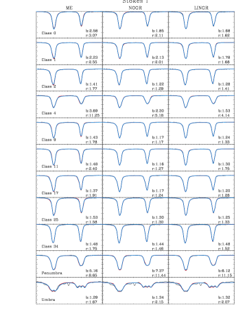
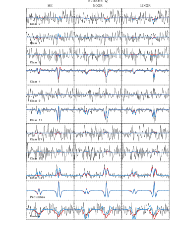
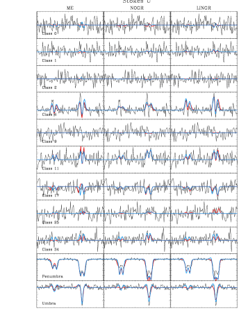
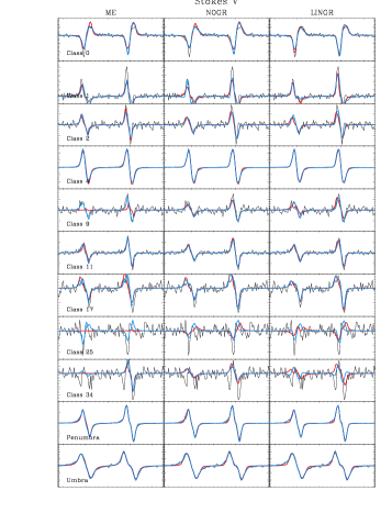
Figure 1.— Maximum a-posteriori fits to the observed Stokes profiles. The black curves are the observed Stokes profiles. The red curves correspond to the models with one magnetic and one non-magnetic components, while the the models with two magnetic components correspond to the blue profiles. We indicate the value of the $\chi^{2}$ for each fit, where the labels $b$ and $r$ refer to “blue” and “red” curves, respectively.

The number of nodes selected for each physical parameter is displayed on Table 3. We fix the number of nodes for the temperature to three, so that the total amount of nodes is six for the two components. In order to test which is the importance of gradients, we consider two options for the LOS velocity and the magnetic field strength. The first one assumes that both quantities take a constant value throughout the atmosphere (models NOGR1+1 and NOGR2, depending on the number of magnetic components). The second one introduces a linear gradient with optical depth (models LINGR1+1 and LINGR2). This opens up the generation of correlated gradients which can potentially generate asymmetries in the Stokes profiles. The number of nodes of the rest of the parameters is kept fixed in both models.

The evidence is calculated with Bayes-LTE, an updated version of Bayes-ME which makes use of an accelerated version of the synthesis core of Nicole (Socas-Navarro, de la Cruz Rodríguez, Asensio Ramos, Trujillo Bueno & Ruiz Cobo, in preparation) and it is also based on the Multinest algorithm. The computation cost of Bayes-LTE is larger than that for Bayes-ME given the large number of evaluations of the model. Each inference with Bayes-LTE takes of the order of 10-20 minutes, being slightly dependent on the number of free parameters. The synthesis engine uses the Hermitian formal solver of Bellot Rubio et al. (1998) and obtains the pressure scale by putting the model in hydrostatic equilibrium using a neural network approach to speed up the calculation. Once synthesized, the lines are convolved with a macroturbulent velocity ($v_{\mathrm{mac}}$) to increase the broadening and produce a better fitting.

5. Results and discussion

5.1. Maximum a-posteriori profiles

Although a potentially large space of parameters is compatible with the observations, the set of parameters that maximize the full multidimensional posterior (maximum a-posteriori; MAP) is of some interest. Since we use flat priors, this solution is equivalent to the one that maximizes the likelihood. Additionally, because we use a Gaussian likelihood, this solution is also equivalent to the one that minimizes the standard $\chi^{2}$ metric used in standard least squares inversion codes. It is important to stress that this solution is not distinguished in any special way from all those that fit the profiles inside the error bars.

Fig. 1 shows the observed Hinode Stokes $I$, $Q$, $U$ and $V$ in black, together with the best fits. The first column corresponds to the fits with Milne-Eddington models, the second to LTE models without gradients along the LOS on the field strength and velocity and the third column to LTE models with gradients. In each column, the red curves correspond to the case of one magnetic component plus a field-free one, while the blue curves refer to the case of two magnetic components. Compared with typical inversion results, one would say that all models are able to do a good job on fitting the full set of profiles. The value of the reduced $\chi^{2}$ metric is shown in each panel, for the 1+1 components red (r) and 2 components blue (b) models. They are displayed again in Tab. 7, where we also show the reduced $\chi^{2}$ ratio between the model with 2 components and the model with 1+1 components. We get small values (close to 1) for all fits, indicating that the fits are acceptable, something that is also relevant from a pure visual inspection. In general, we find a quite systematic decrease of the reduced $\chi^{2}$ when adding a second magnetic component, meaning that the fit is marginally improved. The decrease of the reduced $\chi^{2}$ when adding a second magnetic component is especially large for a few profiles (e.g., class 4 and penumbra). They coincide with the observations with the largest signal-to-noise (SNR). This is an expected behavior in general, consequence of an increase on the number of free parameters, that gives a larger flexibility to the model to fit more details of the observed Stokes profiles. If the SNR of the observation is large, even a relatively good fit obtained with the 1+1 models will produce a large $\chi^{2}$ (this is what happens with class 4 and penumbra), which will be largely reduced by allowing more freedom to the model (using two magnetic components). However, this is not always the case, given that some ratios reported in Tab. 7 are larger than 1. This is the case for classes 0 and 1 in the models with gradients along the LOS. They correspond to profiles with a low polarization amplitude and strong Stokes $V$ asymmetries. In summary, it is hard to say from these fits which model is preferred over the others. Pragmatically, in light of the quality of the fits, one would choose the simplest model. However, the question is whether an improvement in the $\chi^{2}$ is worth the increase in the number of parameters.

Model selection is carried out by comparing evidences, i.e., computing the integral of the posterior over all model parameters. Therefore, the specific values of the parameters is irrelevant. However, for the sake of completeness, we have displayed in Tab. 8 of Appendix B the maximum a-posteriori values of some parameters for all atmospheric models considered and for all observed Stokes profiles. Concerning the magnetic flux density, we see that the inferred value is quite robust to the specific model, except for the umbral profile (in which this quantity is not related to the amplitude of the Stokes $V$ profile) and some IMaX profiles (for which the information is scarce). This is a consequence of the fact that, if the magnetic field strength is not too strong, the magnetic flux density is almost an observable. On the contrary, there is a large variability on the inferred value of the filling factor, something that directly influences the field strength and the inclination. We conclude that the inferred MAP values depend on the selected model and that model selection turns out to be important.

5.2. Model comparison

Once the Bayesian evidence is computed for all models considered, model comparison is just a matter of comparing real numbers and decide on the most probable model following Table 2. Due to the potentially small/large value of the evidence, we reported the value of $\ln p(D|\mathcal{M}_{i})$ in Table 4. We indicate in bold red the model with the largest evidence and in italic red those models that are in competition with the selected model according to the Jeffreys’ scale. Given that we cannot discard the presence of more models compatible with the data, the evidence cannot be considered as an absolute scale. Consequently, we can only compute evidence ratios assuming the same a-priori probability for every model. For this reason, it is also illustrative to consider model comparison in a league framework. This is shown in Fig. 2, where each square indicates the value of the logarithmic evidence ratio obtained from the competition of pairs of models (model in the vertical axis versus model in the horizontal axis). Red colors point out that the model in the left axis is preferred with respect to the model in the horizontal axis. Blue colors are used when the model in the vertical axis is the least preferred one. Light red (blue) colors are associated with the second most (less) probable model. Obviously, only half of the squares contain relevant information, with the other half showing redundant data because they are antisymmetric with respect to the diagonal (with a sign change, equivalent to an inverse in a linear scale for the evidence ratio).

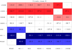
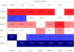
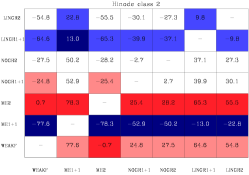
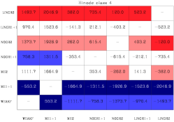
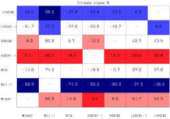
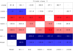
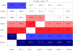
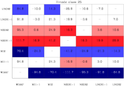
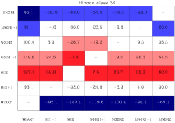
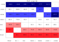
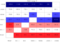
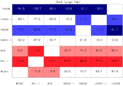
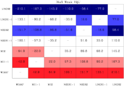
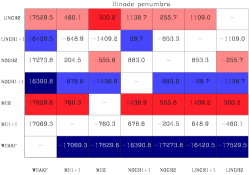
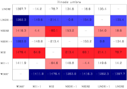
Figure 2.— Logarithmic evidence ratio from each model with respect to the every other model. Models can be compared using these tables if we assume the same a-priori probability for all of them. Each square reports the log evidence ratio between a given model in the vertical axis versus a certain model in the horizontal axis. Red (and light red) indicate the most probable (and second most probable) model in each column, while blue (and light blue) show the less probable (and second less probable) model in each column. Note that these tables are symmetric with respect to the diagonal.

The first thing to note is that there is not a single model that can be considered the “best” for all profiles. A Milne-Eddington model with two magnetic components seems to be the most probable for classes 2, 17 and 34. According to Viticchié et al. (2011), they only represent $\sim$9% of the field-of-view. Classes 0, 1 and 4 favor models with gradients along the LOS in velocity and magnetic field, while classes 9, 11 and 25 favor models without gradients in velocity and magnetic field. A simple weak-field approximation is the model of choice for the majority of IMaX data. Moreover, there is not a single “worst” model, although ME1+1 can be considered not appropriate among the selected models, in general, for explaining our quiet Sun Hinode profiles. This might sound strange given that many spectropolarimetric inversions of Hinode data have been carried out with ME1+1 models. Our results demonstrate that this model is often not preferred by data while the opposite occurs for the ME2 model. The reason has to be found on the presence of asymmetries that a ME1+1 model cannot fit. Obviously, this conclusion is based on the limited number of models that we have considered. If one proposes a different model (there is no difference whether this is a different atmospheric model or one from our selection but with some parameters fixed), it is a matter of computing the evidence to find out if it is preferred by the data.

Another property of our model comparison is that, normally, one model is orders of magnitude much more probable than the rest. Only a few models are really in the position of competing. For instance, for class 9, we see that NOGR1+1 has a log-evidence $\sim$3.4 larger than WEAKF. According to Table 2, there is moderate evidence that NOGR1+1 is preferable to WEAKF. On the contrary, for class 2, we can safely say that there is not a clear preference for ME2 or WEAKF2 (the difference in log-evidence is smaller than 1), with the two models being much more probable than the rest. Other examples can be found by looking at the comparisons of Fig. 2.

Among the quiet Sun profiles, only for classes 0, 1 and 4 the analysis favors models with linear gradients on the field strength and LOS velocity, with class 4 preferring a model with two magnetic components. Classes 0 and 4 have been associated by Viticchié et al. (2011) to the network and they present large amplitudes of circular and linear polarization (class 0 arriving to 2.55% and 0.32% in Stokes $V$ and $L$, respectively, and class 4 reaching 13.2% and 1.30% in Stokes $V$ and $L$, respectively). It is apparent from these results that large SNR ratios are important to favor (or at least allow) more complicated models, especially when the Stokes profiles are inherently complex (asymmetries, several components clearly visible). It is important to point out that the higher SNR is the responsible for the need of increased complexity just because it does not suppress the important details of the Stokes profiles that arise in complex atmospheres. For example, classes 0 and 1 favor LINGR1+1 because the SNR is relatively high and the asymmetry of the Stokes $V$ profiles is clearly visible. Consequently, an increase in the complexity of the model is compensated by the increase on the quality of the fit. On the other side we find, for example, class 2, with small asymmetries and favoring simple models. Additionally, large SNR in Stokes $Q$ and $U$ are also crucial to favor more complicated models. In our case, class 4 have the largest linear polarization signal in the whole set and thus favors complex models even though the asymmetries of Stokes $V$ are small, while classes 0 and 1 are among the ones with the smallest amplitude of linear polarization.

In summary, if the SNR is large, it is possible to increase the number of model parameters if we are able to fit features in the profile that are well above the noise level. This is also consistent with the fact that the MAP fit gives the smallest $\chi^{2}$ for class 0, 1 and 4. Note that, even if the $\chi^{2}$ of class 0 under LINGR1+1 and LINGR2 models is very similar, LINGR1+1 is preferred because of the smaller number of free parameters.

A ME2 model is preferred for all profiles belonging to classes 2, 17 and 34. In general, these classes have linear polarization profiles at or below the noise level (except class 34, which presents clear Stokes $Q$ profiles). Of interest is also the fact that classes 2 and 9, which have the WEAKF model in competition with more complex models, present no detection of linear polarization, while the circular polarization profiles are nearly antisymmetric. The model comparison is suggesting that there is limited information in such profiles and that a WEAKF model can do a good work extracting all available information. A different problem is, obviously, how to interpret this information.

A particularly interesting case is the profile of class 34. The Stokes $V$ signal is clearly $Q$-like as described by Viticchié et al. (2011), giving the idea of several magnetic components with opposite polarities inside the resolution element. The Bayesian analysis suggests that a ME2 model is enough. This seems reasonable, although it is clear that the best fit is not able to correctly fit the two polarities in Stokes $V$. The reason is that the amplitude of Stokes $Q$ is even larger than that of Stokes $V$ and there is not a clear hint of such two components in linear polarization.

Concerning the Hinode profiles observed in sunspots, Table 4 points out that a ME2 model is the most suitable one. This model already produces a very good fit for the two profiles. For the umbra, this preference for ME2 is also understood at the light of the enhanced noise due to the reduced number of photons or the presence of molecular lines not accounted for in the inversion.

The comparison of models for explaining IMaX profiles is also very illuminating. The reduced number of data points strongly suggests that the simple weak-field approximation is the model of choice for explaining the observations among the ones considered in this work. This is especially relevant for the profiles in which either circular or linear polarization (or both simultaneously) is small. This experiment with IMaX data (with the preference for very simple models) shows that complex models with a relatively large number of free parameters are only favored when the number of sampling points in wavelength is large, at least larger than the 25 points of IMaX data. If the sampling is sufficient, the information encoded in the Stokes profiles about the model parameters compensate for the increase in the prior volume of complex models. In case both polarizations are clearly above the noise level, model ME1+1 is preferred, clearly suggesting that some information about the sub-structure in the pixel can be extracted from the observations (apart from the magnetic flux density that can be obtained from the WEAKF approximation). which might be surprising for such a poor spectral sampling. Note that the weak-field approximation allows one to extract very simple quantities from the observables, without allowing for an explicit substructure inside the pixel. We point out that it might be possible to find more complex models but with a reduced number of parameters (smaller than ME1+1) so that it can be preferred by data. The only way to decide on this is to calculate the value of the evidence and compute the evidence ratio.

5.3. Simpler proxies

Given that calculating a reliable estimation of the evidence is computationally very demanding, it is of interest to compare it with simpler proxies used for model comparison. The property of such proxies is that they can be calculated very fast and it is not necessary to perform the multidimensional integral of the evidence. Two of the simple, routinely used proxies are the Bayesian Information Criterion (BIC; Schwarz, 1978) and the Akaike Information Criterion (AIC; Akaike, 1974). Both methods, which are based on the crude approximation of gaussianity of the posterior with respect to the model parameters, are extremely simple to calculate:

$$\mathrm{BIC} = -2\ln\mathcal{L}_{\mathrm{max}}+k\ln N$$ (17)

$$\mathrm{AIC} = -2\ln\mathcal{L}_{\mathrm{max}}+2k,$$ (18)

where $k$ is the number of free parameters of the model, $\mathcal{L}_{\mathrm{max}}$ is the peak value of the likelihood (at the least-squares solution if flat priors are used) and $N$ is the number of observed points. In the case of a Gaussian likelihood, they transform to:

$$\mathrm{BIC} = \chi^{2}_{\mathrm{min}}+k\ln N$$

$$\mathrm{AIC} = \chi^{2}_{\mathrm{min}}+2k,$$ (19)

which can be readly calculated for standard inversion methods based on a least-squares minimization, using the set of parameters $\hat{\mbox{\boldmath$\theta$}}$ that minimize the $\chi^{2}$:

$$\chi^{2}_{\mathrm{min}}=\sum_{j=1}^{M}\left(\frac{y_{j}(\hat{\mbox{\boldmath$\theta$}})-d_{j}}{\sigma_{j}}\right)^{2}.$$ (20)

One of the fundamental problems of these criteria (apart from the assumption of gaussianity of the posterior) is that they penalize all parameters equally, not taking into account situations in which data does not constrain some parameters.

The computed values of the BIC are shown in Table 5. The model with the smallest value of the BIC is the preferred one, contrary to what happens with the evidence. This model is indicated in bold red when it gives the same result using the Bayesian evidence and in blue when it gives a different result. When comparing two models, we have verified that more than 80% of the time the BIC picks up the same model selected by the evidence ratio when dealing with Hinode observations, while this value increases to $\sim$90% when focusing on IMaX profiles. The success rate for selecting the best model using the BIC (as compared with the fully Bayesian case) goes down to 73%. We consider this an indication that the BIC is a very good proxy for the Bayesian evidence. The AIC performs similarly, with BIC being slightly more robust. For instance, the LINGR2 model is preferred by all model comparison methods for the profile associated to Class 4. On the contrary, the weak-field approximation is preferred for Class 9 according to the evidence ratio, while the more complex NOGR2 model is the one of choice according to BIC. Note that, according to the evidence ratio, this is the next preferred model in the hierarchy.

In any case, given the relatively large success rate of BIC for comparison of two models, we suggest anyone carrying out standard inversions to compute the value of the BIC for the selected model. This facilitates model comparison in the future and is able to select the more probable model in a comparison of two with $\sim$80% confidence if our results are used as a calibration. Another application of interest of the proxy is to estimate the minimum number of wavelength points used to sampled the Stokes profiles when observing an unresolved magnetic structure. If one confronts a ME model with one magnetic component and a ME1+1 model to obtain information about the filling-factor, the ME1+1 model will be preferred when BIC(ME1+1) is larger than BIC(ME). With the estimated values of the $\chi^{2}$, one can infer the number of wavelength points to prefer ME1+1.

6. Conclusions

We have presented the first quantitative Bayesian comparison of models used for the interpretation of observed Stokes profiles. Our results suggest that there is not a single model that is suitable for explaining different Stokes profiles in the quiet Sun and in active regions. In essence, the selected model in each case depends on the amount of information encoded in the observations. Simpler models are preferred when the SNR is low or when the spectral sampling is poor because this information is diluted by the noise. Even if the underlying physics is very complex and is producing inherently very complicated Stokes profiles, the presence of noise destroys the information and a simple model is enough to explain them. More complex models are favored when the SNR is large (especially if this is the case for the four Stokes parameters simultaneously) because minute variations of the shape of the Stokes parameters have to be fitted. We stress again that the higher SNR is the responsible for the need of increased complexity just because it does not suppress the important details of the Stokes profiles that arise in complex atmospheres (asymmetries, several components, etc.). Then, we conclude that the complexity of the observed Stokes profiles is the main driver for favoring more elaborate models.

Given that the Bayesian evidence is computationally heavy, we suggest to use the BIC as a trivial output of any inversion code. This will facilitate a more quantitative model comparison in the future, if used as a proxy of the Bayesian evidence. Additionally, the good behavior of the BIC can be used to develop an metainversion scheme in which any of the Eqs. (19) is minimized modifying the values of the free parameters of the models and the models themselves. The result would be a good approximation to the best model that is allowed by the data.

Appendix A Appendix

For the sake of clarity, we write the explicit expressions we have used in each model for the computation of the Stokes profiles.

A.1. Weak-field approximation

In the weak-field approximation, these are the relations between Stokes $Q$, $U$ and $V$ and Stokes $I$ (Landi Degl’Innocenti & Landolfi, 2004):

$$V(\lambda) = -4.67\times 10^{-13}\bar{g}\lambda^{2}B_{\parallel}\frac{\partial I(\lambda)}{\partial\lambda}$$

$$Q(\lambda) = -5.45\times 10^{-26}\bar{G}\lambda^{4}B_{\perp}^{2}\cos 2\chi\frac{\partial^{2}I(\lambda)}{\partial\lambda^{2}}$$

$$U(\lambda) = -5.45\times 10^{-26}\bar{G}\lambda^{4}B_{\perp}^{2}\sin 2\chi\frac{\partial^{2}I(\lambda)}{\partial\lambda^{2}},$$ (A1)

with the wavelength $\lambda$ in Å and the components of the magnetic field vector measured in G. The factor $\bar{g}$ is the effective Landé factor and $\bar{G}$ is the equivalent for linear polarization (e.g., Landi Degl’Innocenti & Landolfi, 2004). The relations at second order for Stokes $Q$ and $U$ are only valid for non-saturated lines. In our modified weak-field approximation, Stokes $I$ is given by Eq. (16) and its derivatives can be computed analytically.

A.2. Milne-Eddington solution

In the Milne-Eddington approximation, the emergent Stokes profiles normalized to the continuum intensity are given by Eqs. (9.110) of Landi Degl’Innocenti & Landolfi (2004), that we rewrite here:

$$\frac{I(\mu)}{I_{c}} = \frac{1}{1+\beta\mu}\left\{1+\beta\mu\Delta^{-1}(1+k_{I})\left[(1+k_{I})^{2}+f_{Q}^{2}+f_{U}^{2}+f_{V}^{2}\right]\right\}$$

$$\frac{Q(\mu)}{I_{c}} = -\frac{\beta\mu}{1+\beta\mu}\Delta^{-1}\left\{(1+k_{I})^{2}k_{Q}-(1+k_{I})(k_{U}f_{V}-k_{V}f_{U})+f_{Q}(k_{Q}f_{Q}+k_{U}f_{U}+k_{V}f_{V})\right\}$$

$$\frac{U(\mu)}{I_{c}} = -\frac{\beta\mu}{1+\beta\mu}\Delta^{-1}\left\{(1+k_{I})^{2}k_{U}-(1+k_{I})(k_{V}f_{Q}-k_{Q}f_{V})+f_{U}(k_{Q}f_{Q}+k_{U}f_{U}+k_{V}f_{V})\right\}$$

$$\frac{V(\mu)}{I_{c}} = -\frac{\beta\mu}{1+\beta\mu}\Delta^{-1}\left\{(1+k_{I})^{2}k_{V}-(1+k_{I})(k_{Q}f_{U}-k_{U}f_{Q})+f_{V}(k_{Q}f_{Q}+k_{U}f_{U}+k_{V}f_{V})\right\},$$ (A2)

where

$$\Delta=(1+k_{I})^{4}+(1+k_{I})^{2}(f_{Q}^{2}+f_{U}^{2}+f_{V}^{2}-k_{Q}^{2}-k_{U}^{2}-k_{V}^{2})-(k_{Q}f_{Q}+k_{U}f_{U}+k_{V}f_{V})^{2}.$$ (A3)

The $k_{i}$ with $i=\{I,Q,U,V\}$ and $f_{i}$ with $i=\{Q,U,V\}$ are the elements of the propagation matrix, as defined in Eq. (9.39) of Landi Degl’Innocenti & Landolfi (2004).

Appendix B Maximum a-posteriori values

Table 8 shows, for all models except the weak-field approximation, the maximum a-posteriori values of: the field strength ($B$), field inclination ($\theta_{B}$), filling factor ($f$) and the magnetic flux density ($\phi$). In these models, the magnetic flux density is computed as $\phi=fB_{1}\cos({[\theta_{B}]}_{1})+(1-f)B_{2}\cos({[\theta_{B}]}_{2})$. Given the special nature of the weak-field model, we only tabulated the magnetic flux density, which is given by $B_{\parallel}$ since there is only one component. Since we use flat priors, the tabulated values coincide with those one would obtain using a standard least-squares fitting of the observed profiles. For the models with two magnetic components, we show the value of $B$ and $\theta_{B}$ in both components. For the models with gradients along the line-of-sight, we tabulate the value at $\log\tau_{5000}=-2$, as a representation of the conditions in the line formation region. We have not shown the error bars to avoid crowding.

Table 8Maximum a-posteriori values for some parameters.

$\phi$ [Mx cm-2]	WEAKF	ME1+1	ME2	NOGR1+1	NOGR2	LINGR1+1	LINGR2
Class 0	$-72.54$	$-62.39$	$-67.83$	$-122.52$	$-145.91$	$-197.62$	$-153.47$
Class 1	$26.71$	$30.89$	$26.67$	$40.37$	$-38.94$	$65.46$	$125.00$
Class 2	$17.80$	$14.02$	$16.97$	$22.64$	$18.65$	$44.93$	$3.74$
Class 4	$676.25$	$734.28$	$708.20$	$501.82$	$615.53$	$514.85$	$601.46$
Class 9	$14.50$	$3.90$	$19.52$	$24.51$	$19.62$	$55.32$	$20.64$
Class 11	$34.95$	$25.71$	$36.91$	$44.36$	$47.33$	$97.59$	$32.41$
Class 17	$16.54$	$15.62$	$19.12$	$23.89$	$27.67$	$46.00$	$23.82$
Class 25	$-9.41$	$0.11$	$-15.85$	$-10.27$	$-1.97$	$-25.50$	$-2.25$
Class 34	$6.28$	$8.28$	$9.36$	$14.51$	$10.73$	$31.93$	$-12.75$
Penumbra	$697.89$	$725.43$	$719.37$	$543.02$	$782.60$	$839.17$	$819.95$
Umbra	$999.86$	$1298.82$	$2532.40$	$2279.34$	$2899.99$	$1703.17$	$2684.40$
IMaX1	$-6.11$	$-11.44$	$-0.18$	$4.64$	$68.47$	$-251.23$	$-1034.43$
IMaX2	$43.97$	$51.38$	$-31.95$	$135.27$	$7.88$	$465.60$	$15.86$
IMaX3	$-18.86$	$-14.42$	$-77.15$	$-281.55$	$-748.89$	$-376.38$	$-514.77$
IMaX4	$-1.39$	$1.42$	$-1.99$	$-34.24$	$125.99$	$0.21$	$1020.42$
$B$ [G]
Class 0	$-$	$1285.24$	$104.79/234.61$	$228.00$	$247.00/82.20$	$367.00$	$357.00/47.90$
Class 1	$-$	$114.62$	$59.03/81.74$	$81.10$	$52.00/96.70$	$143.00$	$68.10/229.00$
Class 2	$-$	$49.73$	$58.35/54.31$	$58.20$	$52.20/48.70$	$103.00$	$36.40/178.00$
Class 4	$-$	$932.46$	$617.19/864.72$	$977.00$	$538.00/819.00$	$814.00$	$844.00/567.00$
Class 9	$-$	$29.80$	$41.18/42.59$	$58.60$	$79.00/44.30$	$102.00$	$106.00/29.90$
Class 11	$-$	$218.74$	$78.82/179.61$	$207.00$	$167.00/161.00$	$395.00$	$155.00/69.30$
Class 17	$-$	$223.00$	$93.53/52.60$	$157.00$	$41.60/151.00$	$248.00$	$134.00/57.30$
Class 25	$-$	$15.98$	$58.29/48.57$	$95.90$	$82.00/54.20$	$191.00$	$213.00/57.00$
Class 34	$-$	$218.70$	$206.35/198.37$	$298.00$	$126.00/337.00$	$488.00$	$545.00/136.00$
Penumbra	$-$	$1337.04$	$1299.85/1337.64$	$1320.00$	$1480.00/930.00$	$1430.00$	$1400.00/1270.00$
Umbra	$-$	$2927.44$	$2888.75/2253.19$	$3030.00$	$2630.00/3810.00$	$2480.00$	$3800.00/2110.00$
IMaX1	$-$	$1369.61$	$59.87/97.49$	$2650.00$	$1870.00/62.70$	$2230.00$	$2170.00/82.90$
IMaX2	$-$	$963.44$	$166.10/34.36$	$381.00$	$259.00/41.20$	$798.00$	$43.00/177.00$
IMaX3	$-$	$435.38$	$140.52/99.94$	$1530.00$	$84.60/3420.00$	$1530.00$	$2260.00/88.70$
IMaX4	$-$	$398.50$	$1.93/51.77$	$572.00$	$13.30/3090.00$	$1890.00$	$102.00/3260.00$
$\theta_{B}$ [deg]
Class 0	$-$	$178.52$	$117.86/137.50$	$149.30$	$158.60/131.60$	$156.40$	$139.50/130.70$
Class 1	$-$	$64.05$	$103.24/63.14$	$40.70$	$61.50/169.80$	$40.30$	$54.10/22.80$
Class 2	$-$	$54.85$	$69.66/87.38$	$52.00$	$65.90/72.50$	$40.40$	$67.80/92.90$
Class 4	$-$	$24.34$	$25.29/25.75$	$15.00$	$43.40/17.80$	$23.80$	$23.60/23.10$
Class 9	$-$	$3.57$	$64.72/46.25$	$48.30$	$71.20/74.90$	$20.00$	$75.20/63.60$
Class 11	$-$	$75.29$	$51.24/79.07$	$71.60$	$80.20/69.10$	$66.20$	$80.00/58.10$
Class 17	$-$	$78.38$	$79.37/59.38$	$72.90$	$76.20/75.10$	$70.10$	$75.50/77.50$
Class 25	$-$	$88.13$	$98.26/125.90$	$104.90$	$84.90/102.10$	$104.30$	$86.00/104.20$
Class 34	$-$	$77.46$	$77.68/89.36$	$84.10$	$87.60/87.10$	$82.20$	$93.90/87.10$
Penumbra	$-$	$51.47$	$53.44/64.39$	$53.00$	$49.80/59.30$	$50.10$	$50.50/59.60$
Umbra	$-$	$17.80$	$21.52/21.43$	$15.90$	$26.20/27.20$	$16.80$	$27.70/26.50$
IMaX1	$-$	$100.67$	$93.36/28.90$	$89.10$	$79.60/96.90$	$109.70$	$186.10/94.70$
IMaX2	$-$	$13.36$	$137.65/128.97$	$47.20$	$112.50/36.90$	$19.80$	$31.50/111.70$
IMaX3	$-$	$103.04$	$137.34/138.23$	$111.70$	$97.00/152.30$	$121.40$	$143.80/96.40$
IMaX4	$-$	$75.73$	$140.44/126.82$	$96.70$	$89.10/40.50$	$89.20$	$92.10/34.00$
$f$
Class 0	$-$	$0.05$	$0.85$	$0.62$	$0.52$	$0.59$	$0.51$
Class 1	$-$	$0.62$	$0.20$	$0.66$	$0.47$	$0.60$	$0.50$
Class 2	$-$	$0.49$	$0.81$	$0.63$	$0.60$	$0.57$	$0.56$
Class 4	$-$	$0.86$	$0.32$	$0.53$	$0.42$	$0.69$	$0.32$
Class 9	$-$	$0.13$	$0.84$	$0.63$	$0.58$	$0.58$	$0.53$
Class 11	$-$	$0.46$	$0.19$	$0.68$	$0.35$	$0.61$	$0.43$
Class 17	$-$	$0.35$	$0.80$	$0.52$	$0.39$	$0.54$	$0.54$
Class 25	$-$	$0.21$	$0.63$	$0.42$	$0.50$	$0.54$	$0.41$
Class 34	$-$	$0.17$	$0.17$	$0.47$	$0.54$	$0.48$	$0.45$
Penumbra	$-$	$0.87$	$0.72$	$0.68$	$0.64$	$0.91$	$0.72$
Umbra	$-$	$0.47$	$0.74$	$0.78$	$0.47$	$0.72$	$0.54$
IMaX1	$-$	$0.05$	$0.96$	$0.11$	$0.22$	$0.33$	$0.48$
IMaX2	$-$	$0.05$	$0.10$	$0.52$	$0.19$	$0.62$	$0.80$
IMaX3	$-$	$0.15$	$0.09$	$0.50$	$0.76$	$0.47$	$0.28$
IMaX4	$-$	$0.01$	$0.98$	$0.51$	$0.95$	$0.01$	$0.62$

References

- Akaike (1974) Akaike, H. 1974, IEEE Trans. Autom. Control, 19, 716
- Anstee & O’Mara (1995) Anstee, S. D., & O’Mara, B. J. 1995, MNRAS, 276, 859
- Asensio Ramos (2009) Asensio Ramos, A. 2009, ApJ, 701, 1032
- Asensio Ramos (2011) Asensio Ramos, A. 2011, in Astronomical Society of the Pacific Conference Series, Vol. 437, Astronomical Society of the Pacific Conference Series, ed. J. R. Kuhn, D. M. Harrington, H. Lin, S. V. Berdyugina, J. Trujillo-Bueno, S. L. Keil, & T. Rimmele, 135–+
- Asensio Ramos & Manso Sainz (2011) Asensio Ramos, A., & Manso Sainz, R. 2011, ApJ, 731, 125
- Asensio Ramos et al. (2007) Asensio Ramos, A., Martínez González, M. J., & Rubiño Martín, J. A. 2007, A&A, 476, 959
- Auer et al. (1977) Auer, L. H., House, L. L., & Heasley, J. N. 1977, Sol. Phys., 55, 47
- Barklem et al. (1998) Barklem, P. S., Anstee, S. D., & O’Mara, B. J. 1998, Publications of the Astronomical Society of Australia, 15, 336
- Beck et al. (2007) Beck, C., Bellot Rubio, L. R., Schlichenmaier, R., & Sütterlin, P. 2007, A&A, 472, 607
- Beck & Rezaei (2009) Beck, C., & Rezaei, R. 2009, A&A, 502, 969
- Bellot Rubio et al. (1998) Bellot Rubio, L. R., Ruiz Cobo, B., & Collados, M. 1998, ApJ, 506, 805
- Bernasconi & Solanki (1996) Bernasconi, P. N., & Solanki, S. K. 1996, Sol. Phys., 164, 277
- Bishop (2006) Bishop, C. M. 2006, Pattern Recognition and Machine Learning (New York: Spinger)
- Borrero et al. (2010) Borrero, J. M., Tomczyk, S., Kubo, M., Socas-Navarro, H., Schou, J., Couvidat, S., & Bogart, R. 2010, Sol. Phys., 35
- Borrero et al. (2007) Borrero, J. M., Tomczyk, S., Norton, A., Darnell, T., Schou, J., Scherrer, P., Bush, R., & Liu, Y. 2007, Sol. Phys., 240, 177
- Carroll & Kopf (2007) Carroll, T. A., & Kopf, M. 2007, A&A, 468, 323
- de la Cruz Rodríguez et al. (2010) de la Cruz Rodríguez, J., Socas-Navarro, H., van Noort, M., & Rouppe van der Voort, L. 2010, MemSAI, 81, 716
- Domínguez Cerdeña et al. (2006) Domínguez Cerdeña, I., Sánchez Almeida, J., & Kneer, F. 2006, ApJ, 646, 1421
- Everitt (1995) Everitt, B. S. 1995, Cluster Analysis (London: Arnold)
- Feroz et al. (2009) Feroz, F., Hobson, M. P., & Bridges, M. 2009, MNRAS, 398, 1601
- Frutiger et al. (2000) Frutiger, C., Solanki, S. K., Fligge, M., & Bruls, J. H. M. J. 2000, A&A, 358, 1109
- Gingerich et al. (1971) Gingerich, O., Noyes, R. W., Kalkofen, W., & Cuny, Y. 1971, Sol. Phys., 18, 347
- Gordon & Trotta (2007) Gordon, C., & Trotta, R. 2007, MNRAS, 382, 1859
- Gregory (2005) Gregory, P. C. 2005, Bayesian Logical Data Analysis for the Physical Sciences (Cambridge: Cambridge University Press)
- Grossmann-Doerth et al. (1988) Grossmann-Doerth, U., Schuessler, M., & Solanki, S. K. 1988, A&A, 206, L37
- Harvey et al. (1972) Harvey, J., Livingston, W., & Slaughter, C. 1972, in Line Formation in the Presence of Magnetic Fields, 227–+
- Jaynes (2003) Jaynes, E. T. 2003, Probability Theory: The Logic of Science (Cambridge: Cambridge University Press)
- Jeffreys (1961) Jeffreys, H. 1961, Theory of Probability (Oxford: Oxford University Press)
- Kass & Raftery (1995) Kass, R., & Raftery, A. 1995, J. Am. Stat. Assoc., 90, 773
- Khomenko et al. (2003) Khomenko, E. V., Collados, M., Solanki, S. K., Lagg, A., & Trujillo Bueno, J. 2003, A&A, 408, 1115
- Kosugi et al. (2007) Kosugi, T., Matsuzaki, K., Sakao, T., Shimizu, T., Sone, Y., Tachikawa, S., Hashimoto, T., Minesugi, K., Ohnishi, A., Yamada, T., Tsuneta, S., Hara, H., Ichimoto, K., Suematsu, Y., Shimojo, M., Watanabe, T., Shimada, S., Davis, J. M., Hill, L. D., Owens, J. K., Title, A. M., Culhane, J. L., Harra, L. K., Doschek, G. A., & Golub, L. 2007, Sol. Phys., 243, 3
- Kupka et al. (1999) Kupka, F., Piskunov, N., Ryabchikova, T. A., Stempels, H. C., & Weiss, W. W. 1999, A&AS, 138, 119
- Lagg et al. (2010) Lagg, A., Solanki, S. K., Riethmüller, T. L., Martínez Pillet, V., Schüssler, M., Hirzberger, J., Feller, A., Borrero, J. M., Schmidt, W., del Toro Iniesta, J. C., Bonet, J. A., Barthol, P., Berkefeld, T., Domingo, V., Gandorfer, A., Knölker, M., & Title, A. M. 2010, ApJl, 723, L164
- Landi Degl’Innocenti & Landi Degl’Innocenti (1973) Landi Degl’Innocenti, E., & Landi Degl’Innocenti, M. 1973, Sol. Phys., 31, 319
- Landi Degl’Innocenti & Landi Degl’Innocenti (1977) —. 1977, A&A, 56, 111
- Landi Degl’Innocenti & Landolfi (2004) Landi Degl’Innocenti, E., & Landolfi, M. 2004, Polarization in Spectral Lines (Kluwer Academic Publishers)
- Lites et al. (2007) Lites, B., Casini, R., Garcia, J., & Socas-Navarro, H. 2007, Mem. Soc. Astron. Ital., 78, 148
- Lites et al. (2001) Lites, B. W., Elmore, D. F., Streander, K. V., Akin, D. L., Berger, T., Duncan, D. W., Edwards, C. G., Francis, B., Hoffmann, C., Katz, N., Levay, M., Mathur, D., Rosenberg, W. A., Sleight, E., Tarbell, T. D., Title, A. M., & Torgerson, D. 2001, in Presented at the Society of Photo-Optical Instrumentation Engineers (SPIE) Conference, Vol. 4498, Proc. SPIE Vol. 4498, p. 73-83, UV/EUV and Visible Space Instrumentation for Astronomy and Solar Physics, ed. O. H. Siegmund, S. Fineschi, & M. A. Gummin, 73
- Lites et al. (2008) Lites, B. W., Kubo, M., Socas-Navarro, H., Berger, T., Frank, Z., Shine, R., Tarbell, T., Title, A., Ichimoto, K., Katsukawa, Y., Tsuneta, S., Suematsu, Y., Shimizu, T., & Nagata, S. 2008, ApJ, 672, 1237
- Lites & Socas-Navarro (2004) Lites, B. W., & Socas-Navarro, H. 2004, ApJ, 613, L600
- MacKay (2003) MacKay, D. J. C. 2003, Information Theory, Inference, and Learning Algorithms (Cambridge University Press)
- Martínez González et al. (2008) Martínez González, M. J., Collados, M., Ruiz Cobo, B., & Beck, C. 2008, A&A, 477, 953
- Martínez Pillet et al. (2011) Martínez Pillet, V., Del Toro Iniesta, J. C., Álvarez-Herrero, A., Domingo, V., Bonet, J. A., González Fernández, L., López Jiménez, A., Pastor, C., Gasent Blesa, J. L., Mellado, P., Piqueras, J., Aparicio, B., Balaguer, M., Ballesteros, E., Belenguer, T., Bellot Rubio, L. R., Berkefeld, T., Collados, M., Deutsch, W., Feller, A., Girela, F., Grauf, B., Heredero, R. L., Herranz, M., Jerónimo, J. M., Laguna, H., Meller, R., Menéndez, M., Morales, R., Orozco Suárez, D., Ramos, G., Reina, M., Ramos, J. L., Rodríguez, P., Sánchez, A., Uribe-Patarroyo, N., Barthol, P., Gandorfer, A., Knoelker, M., Schmidt, W., Solanki, S. K., & Vargas Domínguez, S. 2011, Sol. Phys., 268, 57
- Martínez Pillet et al. (1997) Martínez Pillet, V., Lites, B. W., & Skumanich, A. 1997, ApJ, 474, 810
- Orozco Suárez et al. (2007) Orozco Suárez, D., Bellot Rubio, L. R., del Toro Iniesta, J. C., Tsuneta, S., Lites, B. W., Ichimoto, K., Katsukawa, Y., Nagata, S., Shimizu, T., Shine, R. A., Suematsu, Y., Tarbell, T. D., & Title, A. M. 2007, ApJL, 670, L61
- Piskunov et al. (1995) Piskunov, N. E., Kupka, F., Ryabchikova, T. A., Weiss, W. W., & Jeffery, C. S. 1995, A&AS, 112, 525
- Rees & Semel (1979) Rees, D. E., & Semel, M. D. 1979, A&A, 74, 1
- Ruiz Cobo & del Toro Iniesta (1992) Ruiz Cobo, B., & del Toro Iniesta, J. C. 1992, ApJ, 398, 375
- Sánchez Almeida (1997) Sánchez Almeida, J. 1997, ApJ, 491, 993
- Sánchez Almeida et al. (1989) Sánchez Almeida, J., Collados, M., & del Toro Iniesta, J. C. 1989, A&A, 222, 311
- Sánchez Almeida et al. (1996) Sánchez Almeida, J., Landi Degl’Innocenti, E., Martínez Pillet, V., & Lites, B. W. 1996, ApJ, 466, 537
- Sánchez Almeida & Lites (2000) Sánchez Almeida, J., & Lites, B. W. 2000, ApJ, 532, 1215
- Schwarz (1978) Schwarz, G. E. 1978, The Annals of Statistics, 6, 461
- Semel (1970) Semel, M. 1970, A&A, 9, 152
- Shchukina & Trujillo Bueno (2001) Shchukina, N., & Trujillo Bueno, J. 2001, ApJ, 550, 970
- Sigwarth et al. (1999) Sigwarth, M., Balasubramaniam, K. S., Knölker, M., & Schmidt, W. 1999, A&A, 349, 941
- Skilling (2004) Skilling, J. 2004, in American Institute of Physics Conference Series, Vol. 735, American Institute of Physics Conference Series, ed. R. Fischer, R. Preuss, & U. V. Toussaint, 395
- Skumanich & Lites (1987) Skumanich, A., & Lites, B. W. 1987, ApJ, 322, 473
- Socas-Navarro et al. (1998) Socas-Navarro, H., Ruiz Cobo, B., & Trujillo Bueno, J. 1998, ApJ, 507, 470
- Socas-Navarro et al. (2000) Socas-Navarro, H., Trujillo Bueno, J., & Ruiz Cobo, B. 2000, ApJ, 530, 977
- Solanki et al. (2010) Solanki, S. K., Barthol, P., Danilovic, S., Feller, A., Gandorfer, A., Hirzberger, J., Riethmüller, T. L., Schüssler, M., Bonet, J. A., Martínez Pillet, V., del Toro Iniesta, J. C., Domingo, V., Palacios, J., Knölker, M., Bello González, N., Berkefeld, T., Franz, M., Schmidt, W., & Title, A. M. 2010, ApJL, 723, L127
- Solanki & Montavon (1993) Solanki, S. K., & Montavon, C. A. P. 1993, A&A, 275, 283
- Solanki & Pahlke (1988) Solanki, S. K., & Pahlke, K. D. 1988, A&A, 201, 143
- Solanki & Stenflo (1986) Solanki, S. K., & Stenflo, J. O. 1986, A&A, 170
- Stenflo (1973) Stenflo, J. O. 1973, Sol. Phys., 32, 41
- Stenflo (2010) —. 2010, A&A, 517, A37
- Stenflo (2011) —. 2011, A&A, 529, A42
- Trotta (2008) Trotta, R. 2008, Contemporary Physics, 49, 71
- Viticchié & Sánchez Almeida (2011) Viticchié, B., & Sánchez Almeida, J. 2011, A&A, 530, A14
- Viticchié et al. (2011) Viticchié, B., Sánchez Almeida, J., Del Moro, D., & Berrilli, F. 2011, A&A, 526, A60