Potential integrals on triangles

Abstract

The problem of evaluating potential integrals on planar triangular elements has been addressed using a polar coordinate decomposition. The resulting formulae are general, exact, easily implemented, and have only one special case, that of a field point lying in the plane of the element. Results are presented for the evaluation of the potential and its gradients, where the integrals must be treated as principal values or finite parts, for elements with constant and linearly varying source terms. These results are tested by application to a single triangular element to the evaluation of the potential gradient outside the unit cube. In both cases, the method is shown to be accurate and convergent.

1 INTRODUCTION

A basic operation in any code for the Boundary Element Method (BEM) is the evaluation of potential integrals on elements, whether in the solution of the integral equation, or in the evaluation of field quantities. If we consider the Laplace problem, $\phi$ the potential external to a surface $S$ is given by the integral formulation:

$$\phi(\mathbf{x}) =\int_{S}\frac{\partial\phi_{1}}{\partial n}G(\mathbf{x},\mathbf{x}_{1})-\frac{\partial G(\mathbf{x},\mathbf{x}_{1})}{\partial n}\phi_{1}\,\mathrm{d}S,$$ (1)

where $\mathbf{x}$ indicates position, subscript $1$ variables of integration on the surface $S$ and $n$ the outward pointing normal to the surface. The Green’s function $G$ is given by

$$G(\mathbf{x};\,\mathbf{x}_{1}) =\frac{1}{4\pi R},$$ (2)

$$R =|\mathbf{x}-\mathbf{x}_{1}|.$$

Given the surface potential $\phi$ and gradient $\partial\phi/\partial n$, the potential, and, after differentiation, the gradient(s), can be evaluated at any point in the field. Also, given a boundary condition for $\phi$ and/or $\partial\phi/\partial n$ on $S$, the integral equation can be solved for $\mathbf{x}\in S$.

In any case, the method of solution remains the same: the surface $S$ is divided into elements and suitable shape functions are used to interpolate the potential on these elements. The integral equation is transformed to a linear system in the element potentials, with the influence coefficients determined by the potential generated by each element at each node of the surface mesh. This leads to the requirement to evaluate integrals $I$ and $\partial I/\partial n$ where:

$$I =\iint f(\xi,\eta)G(\mathbf{x},\mathbf{x}_{1}(\xi,\eta))\,\mathrm{d}\xi\,\mathrm{d}\eta,$$ (3)

where $E$ is the surface of an element and $(\xi,\eta)$ is a coordinate system local to $E$.

Numerous techniques have been proposed for the evaluation of $I$ and its derivatives. Many of these have been numerical and have often focussed on the question of evaluating the integral when the evaluation point is close to, but not on, the element [1, 2, 3, for example]. For the Laplace equation, however, it is possible to exactly evaluate the potential integrals analytically and a number of techniques have been published using this approach [4, 5, 6, 7, 8, 9, 10, for example], which has the advantages of being exact and of being less prone to numerical errors introduced by singularities and near-singularities, and, often, more efficient than numerical quadrature.

This paper introduces a method for the evaluation of potential integrals on flat triangular elements, in practice the most common problem encountered in BEM integration. The motivation for this work is to simplify the implementation of the analytical formulae. The numerous results which have been published hereto are, obviously, algebraically equivalent in that they give, or should give, the same answer for any given combination of element and field point. In practice, however, they are not numerically equivalent and, in particular, they have different special cases which must be handled. For example, the formulae of Newman [7], based on the use of Green’s theorem to reduce the surface integral to a sequence of line integrals on the element boundary, have a special case when the field point is collinear with an edge of the triangle. In Salvadori’s work, there are a number of special cases which must be identified and handled separately depending on particular combinations of parameters [10, Figure 5].

In this paper, we present formulae based on a polar coordinate decomposition of the basic integrals which simplifies the integrands to the point where they can be easily evaluated using standard relations and tables and which require handling of only one special case, that when the field point lies in the plane of the element. The method can be generalized to source terms of any order, and to gradients of the potential, which give rise to strongly singular integrands which require treatment as hypersingular integrals.

2 Potential integrals

The approach adopted in developing formulae for the evaluation of potential integrals is similar to that used in previous work: the integral is evaluated on a reference triangle into which the real element can be transformed. In this case, the reference triangle lies in the plane $z=0$, requiring a rotation of the coordinate system, and has one vertex at the projection of the field point into that plane, requiring a decomposition of the original element into a set of subtriangles. We begin by developing formulae for the integrals over the reference triangle, before explaining how these formulae can be applied to general elements.

Figure 1: Reference triangle for quadrature

Figure 3 shows the reference triangle and associated notation. The triangle lies in the plane $z=0$, with one vertex at the origin. The two sides which meet at the origin have length $r_{1}$ and $r_{2}$ and subtend an angle $\Theta$. The third side is given by $x=r_{1}+ay$ with:

$$a =\frac{r_{2}\cos\Theta-r_{1}}{r_{2}\sin\Theta}.$$ (4)

Integrations will be performed by transforming the double integrals in into integrals in the polar coordinate system $(r,\theta)$ centred on the origin. In the triangle coordinate system, the field point is placed at $(0,0,z)$.

The integrals which are required are of the following forms, with the factor $1/4\pi$ suppressed:

$$I =\iint f(x_{1},y_{1})\frac{1}{R}\,\mathrm{d}x_{1}\,\mathrm{d}y_{1},$$ (5a)

$$\frac{\partial I}{\partial z} =-z\iint f(x_{1},y_{1})\frac{1}{R^{3}}\,\mathrm{d}x_{1}\,\mathrm{d}y_{1},$$ (5b)

$$\frac{\partial I}{\partial x} =-\iint f(x_{1},y_{1})\frac{x-x_{1}}{R^{3}}\,\mathrm{d}x_{1}\,\mathrm{d}y_{1},$$ (5c)

$$\frac{\partial^{2}I}{\partial z^{2}} =\iint f(x_{1},y_{1})\left[3\frac{z^{2}}{R^{5}}-\frac{1}{R^{3}}\right]\,\mathrm{d}x_{1}\,\mathrm{d}y_{1},$$ (5d)

$$\frac{\partial^{2}I}{\partial x\partial z} =\iint f(x_{1},y_{1})\frac{3z(x-x_{1})}{R^{5}}\,\mathrm{d}x_{1}\,\mathrm{d}y_{1},$$ (5e)

$$\frac{\partial^{2}I}{\partial x^{2}} =\iint f(x_{1},y_{1})\left[3\frac{(x-x_{1})^{2}}{R^{5}}-\frac{1}{R^{3}}\right]\,\mathrm{d}x_{1}\,\mathrm{d}y_{1},$$ (5f)

$$R^{2} =(x-x_{1})^{2}+(y-y_{1})^{2}+z^{2}.$$

In these integrals, $f(x_{1},y_{1})$ is a source term which varies over the element and subscript $1$ denotes a variable of integration. The basic integral $I$ is the integral over a general triangle in the plane $z=0$ of the Green’s function weighted on the source term. Differentiation with respect to $z$, Equation 5b, corresponds to taking the normal derivative and derivatives with respect to $(x,y,z)$ are used to find the gradient of potential, e.g. the velocity in potential flow problems. Further differentiation yields the hypersingular formulation used in certain applications to avoid numerical difficulties introduced by spurious eigenvalues [11].

The integrals of Equations 5a can be evaluated on the reference triangle of Figure 3 as follows. Considering a general integral:

$$I =\iint f(x_{1},y_{1})R^{\gamma}\,\mathrm{d}x_{1}\,\mathrm{d}y_{1},$$ (6)

$$=\int_{0}^{\Theta}\int_{0}^{\overline{r}(\theta)}f(x_{1},y_{1})R^{\gamma}r\,\mathrm{d}r\mathrm{d}\theta,\quad R^{2}=r^{2}+z^{2},$$ (7)

where

$$\overline{r}(\theta) =\frac{r_{1}}{(1+a^{2})^{1/2}}\frac{1}{\cos(\theta+\phi)},\quad\phi=\tan^{-1}a,$$ (8)

$I$ can be evaluated analytically using tabulated relations.

The first case considered is that of an element with constant source distribution $f(x_{1},y_{1})\equiv 1$:

$$I =\int_{0}^{\Theta}\int_{0}^{\overline{r}(\theta)}R^{\gamma}r\,\mathrm{d}r\mathrm{d}\theta.$$ (9)

Under a change of variables:

$$I =\int_{0}^{\Theta}\int_{|z|}^{\overline{R}(\theta)}R^{\gamma+1}\mathrm{d}R\mathrm{d}\theta,$$ (10)

$$=\frac{1}{\gamma+2}\int_{0}^{\Theta}\overline{R}^{\gamma+2}-|z|^{\gamma+2}\,\mathrm{d}\theta,$$ (11)

$$\overline{R}^{2} =\overline{r}^{2}+z^{2},$$

which can be evaluated with a further change of variables from $\theta$ to $\theta+\phi$:

$$I =\frac{1}{\gamma+2}\left[\beta^{\gamma+2}\int_{\phi}^{\Theta+\phi}\frac{\Delta^{\gamma+2}}{\cos^{\gamma+2}\theta}\,\mathrm{d}\theta-|z|^{\gamma+2}\Theta\right],$$ (12)

where:

$$\Delta^{2} =1-\alpha^{2}\sin^{2}\theta,\quad\alpha^{2}=z^{2}/\beta^{2},\quad\alpha^{\prime}=\left(1-\alpha^{2}\right)^{1/2},\quad\beta^{2}=\frac{r_{1}^{2}+z^{2}(1+a^{2})}{1+a^{2}},$$

$$\overline{r} =\frac{\beta\alpha^{\prime}}{\cos\theta},\quad\text{and}\quad\overline{R}=\beta\frac{\Delta}{\cos\theta}.$$

Integrals of the form of Equation 12 are well understood and extensively tabulated [12, 13]. To simplify the statement of future results, we write the integral as:

$$I =\frac{1}{\gamma+2}\left[\beta^{\gamma+2}\left(I_{0,-\gamma-2}^{(\gamma+2)}(\alpha,\Theta+\phi)-I_{0,-\gamma-2}^{(\gamma+2)}(\alpha,\phi)\right)-|z|^{\gamma+2}\Theta\right],$$ (13)

where

$$I_{m,n}^{(p)}(\alpha,\theta) =\int_{0}^{\theta}\sin^{m}\theta^{\prime}\cos^{n}\theta^{\prime}\Delta^{p}\,\mathrm{d}\theta^{\prime}.$$ (14)

This result is the general form for the integral of any integer power of $R$ over the reference triangle. In particular, subject to triangle decomposition and rotation, it is the only integral required in a BEM which employs constant source elements, as it yields the integrals of $G$ and $\partial G/\partial n$, and includes the integral of $1/R^{3}$ considered by [9]. The only special case which need be handled is that for $z=0$, when the field point lies in the element plane, which will be discussed in Section 2.1.

Higher order elements can be handled in a similar fashion. In the case of elements with linear variation in $f(x_{1},y_{1})$, the integrals to be evaluated are of the form:

$$I =\int_{\phi}^{\Theta+\phi}\int_{0}^{\overline{r}(\theta)}\frac{r\sin^{m}\theta\cos^{n}\theta}{R}r\,\mathrm{d}r\,\mathrm{d}\theta,\quad m+n=1.$$ (15)

In the case $m=0,n=1$, this yields:

$$I =\int_{\phi}^{\Theta+\phi}\cos\theta\int_{0}^{\overline{r}(\theta)}\frac{r^{2}}{R}\,\mathrm{d}r\,\mathrm{d}\theta,$$ (16)

$$=\frac{\beta^{2}\alpha^{\prime}}{2}\int_{\phi}^{\Theta+\phi}\frac{\Delta}{\cos\theta}\,\mathrm{d}\theta-\frac{z^{2}}{4}\left.\log\frac{\Delta+\alpha^{\prime}}{\Delta-\alpha^{\prime}}\sin\theta\right|_{\phi}^{\Theta+\phi}+\frac{z^{2}\alpha^{\prime}}{2}\int_{\phi}^{\Theta+\phi}\frac{\sin^{2}\theta}{\cos\theta}\frac{1}{\Delta}\,\mathrm{d}\theta,$$ (17)

$$=\frac{\beta^{2}\alpha^{\prime}}{2}\left[I_{0,-1}^{(1)}(\alpha,\Theta+\phi)-I_{0,-1}^{(1)}(\alpha,\phi)\right]$$

$$+\frac{z^{2}\alpha^{\prime}}{2}\left[I_{2,-1}^{(-1)}(\alpha,\Theta+\phi)-I_{2,-1}^{(-1)}(\alpha,\phi)\right]-\frac{z^{2}}{4}\left.\log\frac{\Delta+\alpha^{\prime}}{\Delta-\alpha^{\prime}}\sin\theta\right|_{\phi}^{\Theta+\phi},$$ (18)

upon integration by parts. Likewise,

$$\int_{\phi}^{\Theta+\phi}\sin\theta\int_{0}^{\overline{r}(\theta)}\frac{r^{2}}{R}\,\mathrm{d}r\,\mathrm{d}\theta =\frac{\beta^{2}\alpha^{\prime}}{2}\left[I_{1,-2}^{(1)}(\alpha,\Theta+\phi)-I_{1,-2}^{(1)}(\alpha,\phi)\right]$$

$$-\frac{z^{2}\alpha^{\prime}}{2}\left[I_{1,0}^{(-1)}(\alpha,\Theta+\phi)-I_{1,0}^{(-1)}(\alpha,\phi)\right]+\frac{z^{2}}{4}\left.\log\frac{\Delta+\alpha^{\prime}}{\Delta-\alpha^{\prime}}\cos\theta\right|_{\phi}^{\Theta+\phi}.$$ (19)

Finally, higher order elements can be reduced to combinations of the integrals for constant and linear source triangles using the identity $r^{2}=R^{2}-z^{2}$. For second order elements:

$$I =\int_{\phi}^{\Theta+\phi}\sin^{m}\theta\cos^{n}\theta\int_{0}^{\overline{r}}R^{\gamma}r^{3}\,\mathrm{d}r\,\mathrm{d}\theta,\quad m+n=2.$$

$$=\int_{\phi}^{\Theta+\phi}\sin^{m}\theta\cos^{n}\theta\int_{0}^{\overline{r}}R^{\gamma}(R^{2}-z^{2})r\,\mathrm{d}r\,\mathrm{d}\theta,$$ (20)

which reduces to the standard integrals previously introduced:

$$\int_{\phi}^{\Theta+\phi}\sin^{m}\theta\cos^{n}\theta\int_{0}^{\overline{r}}R^{\gamma}r^{3}\,\mathrm{d}r\,\mathrm{d}\theta =\frac{\beta^{\gamma+4}}{\gamma+4}\left[I_{m,n-\gamma-4}^{(\gamma+4)}(\alpha,\Theta+\phi)-I_{m,n-\gamma-4}^{(\gamma+4)}(\alpha,\phi)\right]$$

$$-z^{2}\frac{\beta^{\gamma+2}}{\gamma+2}\left[I_{m,n-\gamma-2}^{(\gamma+2)}(\alpha,\Theta+\phi)-I_{m,n-\gamma-2}^{(\gamma+2)}(\alpha,\phi)\right]$$

$$+|z|^{\gamma+4}\left(\frac{1}{\gamma+2}-\frac{1}{\gamma+4}\right)\left[J_{m,n}(\Theta+\phi)-J_{m,n}(\phi)\right],$$ (21)

$$J_{m,n}(\theta) =\int_{0}^{\theta}\sin^{m}\theta^{\prime}\cos^{n}\theta^{\prime}\,\mathrm{d}\theta^{\prime}.$$ (22)

Explicit expressions for the main results required for constant and linear elements are given in Table 1, with $I_{m,n}^{(p)}$ and $J_{m,n}$ given in the appendix, Tables 3 and 4.

2.1 Field point in plane

The formulae presented above are valid for all field points out of the triangle plane. The case of a point lying in the plane—the only special case which arises—must be handled separately for two reasons. The first is that the formulae presented so far break down numerically unless certain limits are taken explicitly; the second is that a number of the integrals in question are truly singular and must be interpreted as principal value or hypersingular integrals. It is more convenient to handle all of the in-plane cases together using the approach of Brandão [14] who gives a convenient analysis for singular integrals of general form. For example, taking the integral of $1/R^{3}$, and noting that for $z=0$, $r=R$:

$$\int_{0}^{\Theta}\int_{0}^{\overline{r}}\frac{1}{R^{3}}r\,\mathrm{d}r\,\mathrm{d}\theta =\int_{0}^{\Theta}\int_{0}^{\overline{r}}\frac{1}{r^{2}}\,\mathrm{d}r\,\mathrm{d}\theta.$$ (23)

Interpreting the integral in $r$ as a finite-part integral, using Brandão’s method, it can be written:

$$\mathchoice{{\vbox{\hbox{$\textstyle=$}}\kern-7.3611pt}}{{\vbox{\hbox{$\scriptstyle=$}}\kern-4.80557pt}}{{\vbox{\hbox{$\scriptscriptstyle=$}}\kern-3.40279pt}}{{\vbox{\hbox{$\scriptscriptstyle=$}}\kern-2.98611pt}}\!\int_{0}^{\overline{r}}\frac{1}{r^{2}}\mathrm{d}r =-\frac{1}{\overline{r}}=-\frac{\cos\theta}{\beta},$$ (24)

so that:

$$\int_{0}^{\Theta}\mathchoice{{\vbox{\hbox{$\textstyle=$}}\kern-7.3611pt}}{{\vbox{\hbox{$\scriptstyle=$}}\kern-4.80557pt}}{{\vbox{\hbox{$\scriptscriptstyle=$}}\kern-3.40279pt}}{{\vbox{\hbox{$\scriptscriptstyle=$}}\kern-2.98611pt}}\!\int_{0}^{\overline{r}}\frac{1}{R^{3}}\mathrm{d}r\,\mathrm{d}\theta =-\frac{1}{\beta}\left[J_{0,1}(\Theta+\phi)-J_{0,1}(\phi)\right].$$ (25)

For a linear source term:

$$\int_{\phi}^{\Theta+\phi}\int_{0}^{\overline{r}}\frac{r\cos\theta}{R^{3}}r\,\mathrm{d}r\,\mathrm{d}\theta =\int_{\phi}^{\Theta+\phi}\int_{0}^{\overline{r}}\frac{\cos\theta}{r}\,\mathrm{d}r\,\mathrm{d}\theta.$$ (26)

The result of Brandão’s which is applicable is:

$$\mathchoice{{\vbox{\hbox{$\textstyle-$}}\kern-4.86108pt}}{{\vbox{\hbox{$\scriptstyle-$}}\kern-3.25pt}}{{\vbox{\hbox{$\scriptscriptstyle-$}}\kern-2.29166pt}}{{\vbox{\hbox{$\scriptscriptstyle-$}}\kern-1.875pt}}\!\int_{0}^{\overline{r}}\frac{1}{r}\,\mathrm{d}r =\log\overline{r}=-\log\frac{\cos\theta}{\beta},$$ (27)

so that, upon integration by parts:

$$\int_{0}^{\Theta}\mathchoice{{\vbox{\hbox{$\textstyle-$}}\kern-4.86108pt}}{{\vbox{\hbox{$\scriptstyle-$}}\kern-3.25pt}}{{\vbox{\hbox{$\scriptscriptstyle-$}}\kern-2.29166pt}}{{\vbox{\hbox{$\scriptscriptstyle-$}}\kern-1.875pt}}\!\int_{0}^{\overline{r}}\frac{r\cos(\theta+\phi)}{R^{3}}\,\mathrm{d}r\,\mathrm{d}\theta =\left.-\sin\theta\log\frac{\cos\theta}{\beta}\right|_{\phi}^{\Theta+\phi}-\left[J_{2,-1}(\Theta+\phi)-J_{2,-1}(\phi)\right]$$ (28)

and, similarly:

$$\int_{0}^{\Theta}\mathchoice{{\vbox{\hbox{$\textstyle-$}}\kern-4.86108pt}}{{\vbox{\hbox{$\scriptstyle-$}}\kern-3.25pt}}{{\vbox{\hbox{$\scriptscriptstyle-$}}\kern-2.29166pt}}{{\vbox{\hbox{$\scriptscriptstyle-$}}\kern-1.875pt}}\!\int_{0}^{\overline{r}}\frac{r\sin(\theta+\phi)}{R^{3}}\,\mathrm{d}r\,\mathrm{d}\theta =\left.\cos\theta\log\frac{\cos\theta}{\beta}\right|_{\phi}^{\Theta+\phi}+\left[J_{1,0}(\Theta+\phi)-J_{2,-1}(\phi)\right]$$ (29)

Finally, for integrals containing terms $R^{-5}$, the corresponding results are:

$$\int_{0}^{\Theta}\mathchoice{{\vbox{\hbox{$\textstyle=$}}\kern-7.3611pt}}{{\vbox{\hbox{$\scriptstyle=$}}\kern-4.80557pt}}{{\vbox{\hbox{$\scriptscriptstyle=$}}\kern-3.40279pt}}{{\vbox{\hbox{$\scriptscriptstyle=$}}\kern-2.98611pt}}\!\int_{0}^{\overline{r}}\frac{1}{R^{5}}\mathrm{d}r\,\mathrm{d}\theta =-\frac{1}{3\beta^{3}}\left[J_{0,3}(\Theta)-J_{0,3}(\phi)\right]$$ (30)

$$\int_{0}^{\Theta}\mathchoice{{\vbox{\hbox{$\textstyle=$}}\kern-7.3611pt}}{{\vbox{\hbox{$\scriptstyle=$}}\kern-4.80557pt}}{{\vbox{\hbox{$\scriptscriptstyle=$}}\kern-3.40279pt}}{{\vbox{\hbox{$\scriptscriptstyle=$}}\kern-2.98611pt}}\!\int_{0}^{\overline{r}}\frac{r\cos(\theta+\phi)}{R^{5}}\mathrm{d}r\,\mathrm{d}\theta =-\frac{1}{2\beta^{2}}\left[J_{0,3}(\Theta)-J_{0,3}(\phi)\right]$$ (31)

$$\int_{0}^{\Theta}\mathchoice{{\vbox{\hbox{$\textstyle=$}}\kern-7.3611pt}}{{\vbox{\hbox{$\scriptstyle=$}}\kern-4.80557pt}}{{\vbox{\hbox{$\scriptscriptstyle=$}}\kern-3.40279pt}}{{\vbox{\hbox{$\scriptscriptstyle=$}}\kern-2.98611pt}}\!\int_{0}^{\overline{r}}\frac{r\sin(\theta+\phi)}{R^{5}}\mathrm{d}r\,\mathrm{d}\theta =-\frac{1}{2\beta^{2}}\left[J_{1,2}(\Theta)-J_{1,2}(\phi)\right]$$ (32)

Table 1: Summary of main results for constant and linear triangular elements

Integrand	Integral, $z\neq 0$	Integral, $z=0$
$\displaystyle\frac{1}{R}$	$\displaystyle\beta I_{0,-1}^{(1)}-|z|J_{0,0}$	$\displaystyle\beta J_{0,-1}$
$\displaystyle\frac{r\cos(\theta+\phi)}{R}$	$\displaystyle\frac{\beta^{2}\alpha^{\prime}}{2}I_{0,-1}^{(1)}+\frac{z^{2}\alpha^{\prime}}{2}I_{2,-1}^{(-1)}-\frac{z^{2}}{4}\sin\theta\log\frac{\Delta+\alpha^{\prime}}{\Delta-\alpha^{\prime}}$	$\displaystyle\frac{\beta^{2}}{2}J_{0,-1}$
$\displaystyle\frac{r\sin(\theta+\phi)}{R}$	$\displaystyle\frac{\beta^{2}\alpha^{\prime}}{2}I_{1,-2}^{(1)}-\frac{z^{2}\alpha^{\prime}}{2}I_{1,0}^{(-1)}+\frac{z^{2}}{4}\cos\theta\log\frac{\Delta+\alpha^{\prime}}{\Delta-\alpha^{\prime}}$	$\displaystyle\frac{\beta^{2}}{2}J_{1,-2}$
$\displaystyle\frac{1}{R^{3}}$	$\displaystyle-\frac{1}{\beta}I_{0,1}^{(-1)}+\frac{1}{|z|}J_{0,0}$	$\displaystyle-\frac{1}{\beta}J_{0,1}$
$\displaystyle\frac{r\cos(\theta+\phi)}{R^{3}}$	$\displaystyle-\alpha^{\prime}I_{0,1}^{(-1)}-\alpha^{\prime}I_{2,-1}^{(-1)}+\frac{\sin\theta}{2}\log\frac{\Delta+\alpha^{\prime}}{\Delta-\alpha^{\prime}}$	$\displaystyle-\sin\theta\log\frac{\cos\theta}{\beta}-J_{2,-1}$
$\displaystyle\frac{r\sin(\theta+\phi)}{R^{3}}$	$\displaystyle-\frac{\cos\theta}{2}\log\frac{\Delta+\alpha^{\prime}}{\Delta-\alpha^{\prime}}$	$\displaystyle\cos\theta\log\frac{\cos\theta}{\beta}+J_{1,0}$
$\displaystyle\frac{1}{R^{5}}$	$\displaystyle-\frac{1}{3}\left[\frac{1}{\beta^{3}}I_{0,3}^{(-3)}-\frac{1}{|z|^{3}}J_{0,0}\right]$	$\displaystyle-\frac{1}{3\beta^{3}}J_{0,3}$
$\displaystyle\frac{r\cos(\theta+\phi)}{R^{5}}$	$\displaystyle\frac{\alpha^{\prime 3}}{3z^{2}}I_{0,1}^{(-3)}$	$\displaystyle-\frac{1}{2\beta^{2}}J_{0,3}$
$\displaystyle\frac{r\sin(\theta+\phi)}{R^{5}}$	$\displaystyle\frac{\alpha^{\prime 3}}{3z^{2}}I_{1,0}^{(-3)}$	$\displaystyle-\frac{1}{2\beta^{2}}J_{1,2}$
$\displaystyle\frac{r^{2}\cos^{2}(\theta+\phi)}{R^{3}}$	$\displaystyle\beta I_{0,1}^{(1)}+\frac{z^{2}}{\beta}I_{0,3}^{(-1)}-2|z|J_{0,2}$	$\beta J_{0,1}$
$\displaystyle\frac{r^{2}\cos(\theta+\phi)\sin(\theta+\phi)}{R^{3}}$	$\displaystyle\beta I_{1,0}^{(1)}+\frac{z^{2}}{\beta}I_{1,2}^{(-1)}-2|z|J_{1,1}$	$\beta J_{1,0}$
$\displaystyle\frac{r^{2}\sin^{2}(\theta+\phi)}{R^{3}}$	$\displaystyle\beta I_{2,-1}^{(1)}+\frac{z^{2}}{\beta}I_{2,1}^{(-1)}-2|z|J_{2,0}$	$\beta J_{2,-1}$
$\displaystyle\frac{r^{2}\cos^{2}(\theta+\phi)}{R^{5}}$	$\displaystyle-\frac{1}{\beta}I_{0,3}^{(-1)}+\frac{z^{2}}{3\beta^{3}}I_{0,5}^{(-3)}-\frac{2}{3|z|}J_{0,2}$	$\displaystyle-\frac{1}{\beta}J_{0,3}$
$\displaystyle\frac{r^{2}\cos(\theta+\phi)\sin(\theta+\phi)}{R^{5}}$	$\displaystyle-\frac{1}{\beta}I_{1,2}^{(-1)}+\frac{z^{2}}{3\beta^{3}}I_{1,4}^{(-3)}-\frac{2}{3|z|}J_{1,1}$	$\displaystyle-\frac{1}{\beta}J_{1,2}$
$\displaystyle\frac{r^{2}\sin^{2}(\theta+\phi)}{R^{5}}$	$\displaystyle-\frac{1}{\beta}I_{2,1}^{(-1)}+\frac{z^{2}}{3\beta^{3}}I_{2,3}^{(-3)}-\frac{2}{3|z|}J_{2,0}$	$\displaystyle-\frac{1}{\beta}J_{2,1}$

2.2 Integration over general triangles

The preceding sections give exact results for integration over the reference triangle of Figure 3. Any triangular element can be transformed to a combination of triangles of reference shape by the following procedure. It is assumed that the coordinate system has already been transformed so that the triangle lies in the plane $z=0$, a routine operation in evaluation of potential integrals.

Figure 2: Integration over a general triangle (left) by subdivision into three triangles centred at the origin (right). The triangle shown dashed on the right has negative orientation and its contribution is subtracted from that of the other two.

Figure 2 shows a general triangle $123$ and the projection of a field point into the plane of the triangle at point $0$. The system is decomposed into three subtriangles $012$, $023$, and $031$ which are all of reference form. The integral over the triangle is then the sum of the integrals over the subtriangles. In summing the subtriangle integrals, account must be taken of the orientation of the triangles. For example, in Figure 2, the contributions of triangles $012$ and $023$ are added, while that of $031$ is subtracted. The simplest way to incorporate the orientations is to apply it to the calculation of the angle $\Theta$ in Figure 3:

$$\Theta =\pm\cos^{-1}\frac{(\mathbf{x}_{2}-\mathbf{x}_{0}).(\mathbf{x}_{1}-\mathbf{x}_{0})}{|\mathbf{x}_{2}-\mathbf{x}_{0}||\mathbf{x}_{1}-\mathbf{x}_{0}|},$$ (33)

where the sign is chosen to agree with the orientation (signed area) of the triangle. Orientations are computed using Shewchuk’s robust adaptive predicates [15].

For constant source elements, the subtriangle integrals can be summed directly. When there is a variation in the source term, two rotations must be applied, one by angle $\phi$, Equation 8, and one by angle $\psi$:

$$\psi=\tan^{-1}\frac{y_{1}-y_{0}}{x_{1}-x_{0}},$$ (34)

where subscript $0$ refers to the field point and subscript $1$ to the first vertex of the triangle. Assembling these rotations gives, for the linear source:

$$\left[\begin{array}[]{l}\displaystyle\iint\frac{x_{1}}{R}\mathrm{d}x_{1}\,\mathrm{d}y_{1}\\ \displaystyle\iint\frac{y_{1}}{R}\mathrm{d}x_{1}\,\mathrm{d}y_{1}\end{array}\right] =\sum_{i}\left[\begin{array}[]{rr}\cos\psi_{i}&-\sin\psi_{i}\\ \sin\psi_{i}&\cos\psi_{i}\end{array}\right]\left[\begin{array}[]{rr}\cos\phi_{i}&\sin\phi_{i}\\ -\sin\phi_{i}&\cos\phi_{i}\end{array}\right]\left[\begin{array}[]{l}\displaystyle\int_{\phi}^{\phi+\Theta}\int_{0}^{\overline{r}}\frac{r\cos(\theta+\phi)}{R}r\,\mathrm{d}r\,\mathrm{d}\theta\\ \displaystyle\int_{\phi}^{\phi+\Theta}\int_{0}^{\overline{r}}\frac{r\sin(\theta+\phi)}{R}r\,\mathrm{d}r\,\mathrm{d}\theta\end{array}\right]$$ (43)

$$+\left[\begin{array}[]{r}x_{0}\\ y_{0}\end{array}\right]\int_{\phi}^{\phi+\Theta}\int_{0}^{\overline{r}}\frac{1}{R}r\,\mathrm{d}r\,\mathrm{d}\theta,$$ (46)

where subscript $i=1,2,3$ refers to the subtriangles into which the element is decomposed.

2.3 Summary of algorithm

In summary, given a triangle lying in the plane $z=0$ and a field point at some general position, the potential integrals can be computed as follows:

1. check if the field point lies in the plane $z=0$;

2. decompose the triangle into subtriangles as in Figure 2;

3. for each triangle $i=1,2,3$:

   1. compute the orientation (signed area) of the triangle;

   2. if the orientation is not zero, calculate $a$, $r_{1}$, $r_{2}$, $\Theta_{i}$, and $\phi_{i}$ using Equations 4 and 8, taking account of the orientation;

   3. evaluate the required integrals using the appropriate formulae of Table 1, depending on whether or not $z=0$;

   4. if required, apply the rotations of Equation 46.

4. sum the results from the three subtriangles.

If necessary, e.g. for the computation of gradients, a further rotation can then be applied to return to the global coordinate system.

3 Numerical tests

Two main sets of tests have been performed to check the formulae presented. The first consists of the evaluation of sample integrals on a single triangle, with field points chosen to be representative of the cases likely to cause numerical difficulties. The second is a test of the estimation of the gradient of a known potential field outside the unit cube. This tests the method in a BEM code and assesses its ability to accurately integrate the strongly singular integrands which arise in computing gradients.

3.1 Integrals on a sample triangle

Figure 3: Reference triangle for test of integration procedures. Points 1–5 are the projections onto the triangle plane of the field points. Points are 1: $(-0.5,-0.1)$; 2: $(0.1,0.1)$; 3: $(0.1,-0.101)$; 4: $(-0.1,-0.099)$; 5: $(0.3,0.2)$.

The triangular element for the first test is shown in Figure 3. The test integrals were evaluated at a range of values of $z$, over five different positions in the triangle plane, shown in Figure 3. For $I_{1}$ and $I_{2}$, $0\leq z\leq 1$, while for $I_{3}$, $1/8\leq z\leq 1$, since the numerical integration routine will not give correct results at $z=0$. These points were chosen to test for the cases most likely to be encountered in practice. Point 1 is directly over a triangle vertex; point 2 lies inside the triangle boundary; points 3 and 4 lie near the triangle boundary but just inside and outside it respectively; point 5 is well separated from the element. Three basic integrals were evaluated:

$$I_{1} =\iint\frac{L_{i}(\xi,\eta)}{4\pi R}\,\mathrm{d}x_{1}\,\mathrm{d}y_{1},$$ (47a)

$$I_{2} =z\iint\frac{L_{i}(\xi,\eta)}{4\pi R^{3}}\,\mathrm{d}x_{1}\,\mathrm{d}y_{1}=-\frac{\partial I_{1}}{\partial n},$$ (47b)

$$I_{3} =\iint\frac{L_{i}(\xi,\eta)}{4\pi R^{5}}\,\mathrm{d}x_{1}\,\mathrm{d}y_{1},$$ (47c)

where $L_{i}(\xi,\eta)$, $i=1,2,3$ are the linear shape functions for the triangle:

$$L_{1} =1-\xi-\eta,\quad L_{2}=\xi,\quad L_{3}=\eta.$$ (48)

For comparison with a numerical method, the integrals were also evaluated using the approach of Hayami [3]. The error $\epsilon_{j}$, $j=1,2,3$, is calculated as the maximum of the differences between the numerical and analytical values for $I_{j}$, for each value of $i$, and is shown in Table 2.

Table 2: Errors in evaluation of integrals for triangle of Figure 3

Point	$\epsilon_{1}$	$\epsilon_{2}$	$\epsilon_{3}$
1	$1.5\times 10^{-14}$	$1.4\times 10^{-12}$	$4.4\times 10^{-10}$
2	$2.5\times 10^{-11}$	$1.4\times 10^{-09}$	$4.3\times 10^{-07}$
3	$4.9\times 10^{-04}$	$6.9\times 10^{-09}$	$2.4\times 10^{-06}$
4	$1.7\times 10^{-05}$	$6.8\times 10^{-09}$	$2.4\times 10^{-06}$
5	$4.6\times 10^{-14}$	$2.9\times 10^{-12}$	$8.9\times 10^{-10}$

From Table 2, the accuracy of the method is clearly displayed: the errors are comparable to machine precision, with the exception of the hypersingular case for points 2–4, where the numerical integration routine would be expected to break down, and for points 3 and 4 for $I_{1}$, where the numerical method has difficulty in dealing with the very slender triangle between the evaluation point and the lower vertices of the triangle.

3.2 Potential gradient calculation

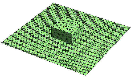
Figure 4: Unit cube and gradient test surface

The second test was an evaluation of the gradient of a potential field outside the unit cube. The evaluation method was implemented in the free BEM code BEM3D [16], based on the GTS triangulated surface library [17], and used to find the gradient of the potential outside a unit cube centred on the origin, Figure 4. The boundary condition for potential and potential gradient was imposed using a point source placed inside the cube at $(1/4,1/4,1/4)$ and the field was evaluated as the gradient of Equation 1. The measure of error was the maximum difference in any of the three components of the gradient on a $32\times 32$ grid $-2\leq x\leq 2,-2\leq y\leq 2,z=0$:

$$\epsilon =\max\left|\left.\frac{\partial\phi}{\partial x_{i}}\right|_{\text{computed}}-\left.\frac{\partial\phi}{\partial x_{i}}\right|_{\text{exact}}\right|/\max|\nabla\phi|.$$ (49)

The cube mesh was generated using gmsh [18], with the discretization length $h$ varied as a parameter.

Figure 5: Error versus discretization length for gradient of Laplace potential outside the unit cube. Symbols: computed error; solid line: $\epsilon=2.72h^{2.12}$.

The resulting error is shown in Figure 5 and demonstrates second order convergence with $h$, as might be expected for linear elements. Again, the accuracy of the method is confirmed.

4 Conclusions

A method and explicit formulae for the exact integration of potential integrals on planar triangular elements in the boundary element method has been presented. The formulae are easily implemented using standard operations and testing against numerical quadrature has shown them to be accurate and, when implemented in a BEM code, convergent.

Appendix A Basic integrals

Expressions for $I_{m,n}^{(p)}$ and $J_{m,n}$ can be found in standard tables [12, 13] and are listed in Tables 3 and 4. Also, where $I_{m,n}^{(-3)}$ is not given explicitly, it can be expressed in terms of lower order integrals [12, 2.581.2]:

$$I_{m,n}^{(-3)}(\alpha,\theta) =\frac{\sin^{m-1}\theta\cos^{n-1}\theta}{\alpha^{2}\Delta}-\frac{m-1}{\alpha^{2}}I_{m-2,n}^{(-1)}(\alpha,\theta)+\frac{n-1}{\alpha^{2}}I_{m,n-2}^{(-1)}(\alpha,\theta)$$ (50)

Table 3: $I_{mn}^{(p)}(\theta)$, constant of integration omitted

$p$	$m$	$n$	$I_{mn}^{(p)}$
-3	0	1	$\displaystyle\frac{\sin\theta}{\Delta}$
	1	0	$\displaystyle-\frac{1}{\alpha^{\prime 2}}\frac{\cos\theta}{\Delta}$
	0	3	$\displaystyle-\frac{\alpha^{\prime 2}}{\alpha^{2}}\frac{\sin\theta}{\Delta}+\frac{1}{\alpha^{3}}\sin^{-1}(\alpha\sin\theta)$
-1	0	1	$\displaystyle\frac{1}{\alpha}\sin^{-1}(\alpha\sin\theta)$
	1	0	$\displaystyle-\frac{1}{\alpha}\ln(\alpha\cos\theta+\Delta)$
	2	-1	$\displaystyle\frac{1}{2\alpha^{\prime}}\ln\frac{\Delta+\alpha^{\prime}\sin\theta}{\Delta-\alpha^{\prime}\sin\theta}-\frac{1}{\alpha}\sin^{-1}(\alpha\sin\theta)$
1	0	-1	$\displaystyle\frac{\alpha^{\prime}}{2}\ln\frac{\Delta+\alpha^{\prime}\sin\theta}{\Delta-\alpha^{\prime}\sin\theta}+\alpha\sin^{-1}(\alpha\sin\theta)$
	2	-1	$\displaystyle-\frac{\Delta\sin\theta}{2}+\frac{2\alpha^{2}-1}{2\alpha}\sin^{-1}(\alpha\sin\theta)+\frac{\alpha^{\prime}}{2}\ln\frac{\Delta+\alpha^{\prime}\sin\theta}{\Delta-\alpha^{\prime}\sin\theta}$
	1	-2	$\displaystyle\frac{\Delta}{\cos\theta}-\alpha\ln(\alpha\cos\theta+\Delta)$
	1	0	$\displaystyle-\frac{\Delta\cos\theta}{2}-\frac{1}{2}\frac{\alpha^{\prime 2}}{\alpha}\ln(\alpha\cos\theta+\Delta)$

Table 4: $J_{mn}(\theta)$, constant of integration omitted

$m$	$n$	$J_{mn}$
0	0	$\theta$
0	-1	$\displaystyle\ln\frac{1+\sin\theta}{1-\sin\theta}$
0	1	$\displaystyle\sin\theta$
1	0	$\displaystyle-\cos\theta$
0	3	$\displaystyle\sin\theta-\frac{1}{3}\sin^{3}\theta$
1	-2	$\displaystyle\frac{1}{\cos\theta}$
1	2	$\displaystyle-\frac{\cos^{3}\theta}{3}$
2	-1	$\displaystyle-\sin\theta+\ln\left(\frac{\pi}{4}+\frac{\theta}{2}\right)$

References

• [1] J. C. F. Telles. A self-adaptive co-ordinate transformation for efficient numerical evaluation of general boundary element integrals. International Journal for Numerical Methods in Engineering, 24:959–973, 1987.
• [2] Ken Hayami and Hideki Matsumoto. A numerical quadrature for nearly singular boundary element integrals. Engineering Analysis with Boundary Elements, 13:143–154, 1994.
• [3] Ken Hayami. Variable transformations for nearly singular integrals in the boundary element method. Publications of the Research Institute for Mathematical Sciences, 41:821–842, 2005.
• [4] Ephraim E. Okon and Roger F. Harrington. The potential due to a uniform source distribution over a triangular domain. International Journal for Numerical Methods in Engineering, 18:1401–1419, 1982.
• [5] Ephraim E. Okon and Roger F. Harrington. The potential integral for a linear distribution over a triangular domain. International Journal for Numerical Methods in Engineering, 18:1821–1828, 1982.
• [6] E. E. Okon. Potential integrals associated with quadratic distributions in a triangular domain. International Journal for Numerical Methods in Engineering, 21:197–209, 1985.
• [7] J. N. Newman. Distributions of sources and normal dipoles over a quadrilateral panel. Journal of Engineering Mathematics, 20:113–126, 1986.
• [8] S. Nintcheu Fata. Explicit expressions for 3D boundary integrals in potential theory. International Journal for Numerical Methods in Engineering, 78:32–47, 2009.
• [9] A. Carini and A. Salvadori. Analytical integrations in 3D BEM: preliminaries. Computational Mechanics, 28:177–185, 2002.
• [10] A. Salvadori. Analytical integrations in 3D BEM for elliptic problems: Evaluation and implementation. International Journal for Numerical Methods in Engineering, 84:505–542, 2010.
• [11] A. J. Burton and G. F. Miller. The application of integral equation methods to the numerical solution of some exterior boundary-value problems. Proceedings of the Royal Society of London. A., 323:201–210, 1971.
• [12] I. Gradshteyn and I. M. Ryzhik. Table of integrals, series and products. Academic, London, 5th edition, 1980.
• [13] A. P. Prudnikov, Yu. A. Brychkov, and O. I. Marichev. Integraly i ryady: Tom 1 Elemntarnye funktsii (Integrals and series: Volume 1 Elementary functions). Fizmatlit, Moscow, 2nd edition, 2003.
• [14] Mauricio Pazini Brandão. Improper integrals in theoretical aerodynamics: The problem revisited. AIAA Journal, 25(9):1258–1260, September 1987.
• [15] Jonathan Richard Shewchuk. Robust adaptive floating-point geometric predicates. In Proceedings of the Twelfth Annual Symposium on Computational Geometry, pages 141–150. Association for Computing Machinery, May 1996.
• [16] Michael Carley. BEM3D: A free three-dimensional boundary element library. http://www.paraffinalia.co.uk/Software/bem3d.shtml, 2009–2012. accessed 15 January 2012.
• [17] Stephane Popinet. GTS: GNU Triangulated Surface library. http://gts.sourceforge.net/, 2000–2004.
• [18] Christophe Geuzaine and Jean-François Remacle. Gmsh: a three-dimensional finite element mesh generator with built-in pre- and post-processing facilities. International Journal for Numerical Methods in Engineering, 79(11):1309–1331, 2009.