Initial data sets with ends of cylindrical type:
I. The Lichnerowicz equation

Abstract

We construct large classes of vacuum general relativistic initial data sets, possibly with a cosmological constant $\Lambda\in\mathbb{R}$, containing ends of cylindrical type.

1 Introduction

There are several classes of general relativistic initial data sets which have been extensively studied, including:

1. compact manifolds,

2. manifolds with asymptotically flat ends, and

3. manifolds with asymptotically hyperbolic ends.

There is another type of interesting asymptotic geometry which appears naturally in general relativistic studies, namely:

1. manifolds with ends of cylindrical type.

The problem is then to construct solutions of the general relativistic vacuum constraint equations:

$$\begin{split}&R(g)=2\Lambda+|K|_{g}^{2}-({\mbox{\rm tr\,}}_{g}K)^{2}\\ &\mbox{div}_{g}\,K+\nabla{\mbox{\rm tr\,}}_{g}K=0\;,\end{split}$$ (1.1)

so that the initial data set $(M,g,K)$ contains ends of cylindrical type.

The simplest such solution is the cylinder $\mathbb{R}\times S^{n-1}$ with the standard product metric and with extrinsic curvature tensor $K\equiv 0$. Its vacuum development when the cosmological constant $\Lambda$ is zero is the interior Schwarzschild solution, and when $\Lambda>0$ the Nariai solution. When $\Lambda=0$, other examples are provided by the static slices of extreme Kerr solutions or of the Majumdar-Papapetrou solutions (see Appendix B), as well as those CMC slices in the Schwarzchild-Kruskal-Szekeres space-times which are asymptotic to slices of constant area radius $r<2m$.

Data of this type have already been studied in [17, 18, 24, 15, 49, 50, 25, 5], but no systematic analysis exists in the literature. The object of this paper is to initiate such a study. As is already known from the study of the Yamabe problem on manifolds with ends of cylindrical type, it is natural and indeed necessary to consider not only initial data sets where the metric is asymptotically cylindrical, but also metrics which are asymptotically periodic. For the constant scalar curvature problem, these are asymptotic to the Delaunay metrics, cf. [7, 13, 14, 34, 42]), which in the relativistic setting are the metrics induced on the static slices of the maximally extended Schwarzschild-de Sitter solutions. We refer also to [46, 43, 42, 41, 39, 40, 34, 44, 7, 13, 14, 8, 9, 37] for the construction, and properties, of complete constant positive scalar curvature metrics with asymptotically Delaunay ends. Exactly periodic solutions of (1.1) are obtained by lifting solutions of the constraint equations from $S^{1}\times N$ to the cyclic cover $\mathbb{R}\times N$, where $N$ is any compact manifold. In particular, the lifts to $\mathbb{R}\times S^{2}$ of initial data sets for the Gowdy metrics on $S^{1}\times S^{2}$ provide a large family of non-CMC periodic solutions.

For all of these reasons, we include in our general considerations

1. manifolds with asymptotically periodic ends.

More generally still, some of the analysis here applies to the class of

1. manifolds with cylindrically bounded ends.

By this we mean that on each end, the metric is uniformly equivalent to a cylindrical metric, with uniform estimates on derivatives up to some order. This is a particularly useful category because it includes not only metrics which are asymptotically cylindrical or periodic, but also metrics which are conformal to either of these types, with a conformal factor which is bounded above and below. In fact, the solutions to (1.1) we obtain starting from background asymptotically cylindrical or periodic metrics are usually of this conformally asymptotically cylindrical or periodic type, so it is quite natural to include this broader class into our considerations to the extent possible. We shall often refer to the geometries in cases 4)-6) as being ends of cylindrical type.

Finally, we shall incorporate this study of solutions with ends of cylindrical type into the more familiar study of solutions of (1.1) with ends which are asymptotically Euclidean or asymptotically hyperbolic. In other words, we are interested in finding solutions with ends of different types, some cylindrical and others asymptotically Euclidean or asymptotically hyperbolic. There is a slight generalization of asymptotically Euclidean geometry which is easy to include, namely

1. manifolds with asymptotically conical ends.

This means that the metric on that end is asymptotic to $dr^{2}+r^{2}h$ as $r\to\infty$, where $(N,h)$ is a compact Riemannian manifold. The standard asymptotically Euclidean case occurs when $N=S^{n-1}$ and $h$ is the standard round metric. For simplicity, we use either of these designations, i.e. either asymptotically Euclidean or conic, with the understanding that the results apply to both unless explicitly stated otherwise.

The reader should keep in mind that there is experimental evidence suggesting that we live in a world with strictly positive cosmological constant $\Lambda$ [51, 45, 33], whence the need for a better understanding of the space of solutions of Einstein equations with $\Lambda>0$. In the simplest time-symmetric setting, this leads to the study of manifolds with constant positive scalar curvature in which case, as discussed above, manifolds with ends of cylindrical type appear as natural models. We note that the topology of manifolds carrying complete metrics with positive scalar curvature, bounded sectional curvature and injectivity radius bounded away from zero has been recently classified in [6] using Ricci flow. Any such manifold which is also orientable is a connected sum of copies of $S^{1}\times S^{2}$ and quotients of $S^{3}$ by finite rotation groups; if the manifold is noncompact, then infinite connected sums may occur.

We shall be using the standard conformal method. This is well understood within the class of CMC initial data on compact manifolds [29], at least when the trace $\tau=g^{ij}K_{ij}$ is large enough, in the sense that

$$\tau^{2}\geq\frac{2n}{(n-1)}\Lambda\;.$$ (1.2)

(There are now a number of results in various geometric settings which relax this condition, see [27, 28, 38, 16, 22, 31] and references therein, but this more general problem is still far from settled.) Since this paper is meant to be a preliminary general investigation of the constraint equations for cylindrical geometries, we shall be assuming the condition (1.2) in almost all of the results below. Note that in the special case where $K=\frac{\tau}{n}g$, i.e. the extrinsic curvature is pure trace, insertion of (1.2) into (1.1) yields $R(g)\leq 0$. We are not, however, assuming that $K$ is pure-trace nor that $R(g)\leq 0$ unless explicitly indicated otherwise in some cases below.

We recall that for the constant scalar curvature equation, the barrier method, i.e. the use of sub- and supersolutions, is effective when $R(g)\leq 0$; but that when studying noncompact metrics with constant positive scalar curvature it seems to be necessary to use more intricate parametrix-based methods. Because we do assume (1.2) throughout, we are able to use barrier methods in all that follows. We hope to return in future work to the study of (1.1) for manifolds with ends of cylindrical type where (1.2) does not hold and more complicated analytic methods become necessary.

Our focus here is specifically on the Lichnerowicz equation and not the vector constraint equation. Thus in all that follows we simply assume the existence of $TT$ tensors satisfying various asymptotic conditions. Large classes of such tensors are constructed in an accompanying paper [12]. Alternatively, we could also use in some of our results the compactly supported $TT$ tensors constructed in [19]. Many of the results below are phrased using a somewhat general form of the semilinear elliptic scalar constraint equation, and depend only on certain structural features of the Lichnerowicz equation. In particular, we carry out our investigations without assuming that $d\tau=0$, in hopes that our results can, for example, be adapted for use as in [16, 27]. The results here directly provide solutions of the constraint equations only when $\tau$ is constant.

As a guide to the rest of the paper, the next section reviews the Lichnerowicz equation and its behaviour under conformal rescaling, as well as the monotone iteration scheme and the method of sub- and supersolutions. Section 3 describes various solutions of the Lichnerowicz-type equation which depend on only one variable. There are several cases, depending on the signs, which we assume to be constant, of the different coefficient functions. These are the basic models for the geometry of solutions on ends of cylindrical type.

We call special attention to the class of periodic solutions which generalize the constant scalar curvature Delaunay metrics. These constraint Delaunay solutions, which arise when the TT tensor has constant nonzero norm, should be regarded as deformations of the standard Delaunay solutions. Continuing on, the main analysis is contained in §4. We separate this into two cases, depending on whether the scalar curvature of the initial metric is nonnegative, or else strictly negative outside a compact set. We describe the relationships of these conditions with the sign of the Yamabe invariant of the noncompact manifold, and prove a number of existence theorems for solutions of (1.1) with ends of cylindrical type in these two cases. The following two sections indicate how to obtain solutions which have some cylindrical ends and others which are either asymptotically hyperbolic (§5) or else asymptotically conical (§6).

In all cases, the existence proofs rely on construction of suitable barrier functions. Appendix A contains a proof of existence of solutions of the Lichnerowicz-type equation using the monotone iteration scheme and assuming the existence of suitable barrier functions, without any completeness of uniformity assumptions. We also describe there some generalities about barrier functions and give examples for the special geometries of interest here. Finally, Appendix B gives a number of examples from the relativity literature where initial data sets with ends of cylindrical type are encountered.

2 The Lichnerowicz equation

Fix a cosmological constant $\Lambda$ and a symmetric tensor field $\tilde{L}$ on a Riemannian manifold $(M,{\tilde{g}})$, as well as a smooth bounded function $\tau$. This last function represents the trace of the extrinsic curvature tensor. As noted earlier, we do not assume that $d\tau=0$. We also do not need to assume that $\tilde{L}$ is transverse-traceless, though it is in the application to the constraint equations. To simplify notation, set

$${\tilde{\sigma}}^{2}:=\frac{n-2}{4(n-1)}|\tilde{L}|_{\tilde{g}}^{2}\;,\quad\beta:=\left[\frac{n-2}{4n}\tau^{2}-\frac{n-2}{2(n-1)}\Lambda\right],$$ (2.1)

which is convenient since only these quantities, rather than $\tilde{L}$, $\tau$ or $\Lambda$, appear in the constraint equations. The symbol ${\tilde{\sigma}}^{2}$ is meant to remind the reader that this function is nonnegative, but is slightly misleading since ${\tilde{\sigma}}^{2}$ may not be the square of a smooth function. All of these functions are as regular as the metric $g$ and the extrinsic curvature $K$.

We shall be studying the Lichnerowicz equation

$$\Delta_{\tilde{g}}{\tilde{\phi}}-\frac{n-2}{4(n-1)}\tilde{R}{\tilde{\phi}}=\beta{\tilde{\phi}}^{(n+2)/(n-2)}-{\tilde{\sigma}}^{2}{\tilde{\phi}}^{(2-3n)/(n-2)},$$ (2.2)

which corresponds to the first of the two equations in (1.1). We write it more simply as

$$L_{{\tilde{g}}}{\tilde{\phi}}=\beta{\tilde{\phi}}^{\alpha}-{\tilde{\sigma}}^{2}{\tilde{\phi}}^{-\gamma}.$$ (2.3)

Here and for the rest of the paper, $L_{\tilde{g}}$ denotes the conformal Laplacian,

$$L_{{\tilde{g}}}=\Delta_{{\tilde{g}}}-\frac{n-2}{4(n-1)}\tilde{R},$$

and we also always set

$$c(n)=\frac{n-2}{4(n-1)},\quad\alpha=\frac{n+2}{n-2}\quad\mbox{and}\quad\gamma=\frac{3n-2}{n-2}.$$ (2.4)

An important property of (2.3) is the following conformal transformation property. Suppose that $\hat{g}=u^{\frac{4}{n-2}}{\tilde{g}}$. It is well known that for any function $\hat{\phi}$ it holds that

$$L_{{\tilde{g}}}(u\hat{\phi})=u^{\alpha}L_{\hat{g}}\hat{\phi},$$

where $L_{\hat{g}}$ is the conformal Laplacian associated to $\hat{g}$. Thus if we set ${\tilde{\phi}}=u\hat{\phi}$ into (2.3), this last equation becomes

$$u^{\alpha}L_{\hat{g}}\hat{\phi}=\beta u^{\alpha}\hat{\phi}^{\alpha}-{\tilde{\sigma}}^{2}u^{-\gamma}\hat{\phi}^{-\gamma}.$$

Dividing by $u^{\alpha}$ and defining

$$\hat{\sigma}^{2}=u^{-\gamma-\alpha}{\tilde{\sigma}}^{2},$$ (2.5)

then we have simply that

$$L_{\hat{g}}\hat{\phi}=\beta\hat{\phi}^{\alpha}-\hat{\sigma}^{2}\hat{\phi}^{-\gamma}.$$ (2.6)

Note in particular that while ${\tilde{\sigma}}^{2}$ transforms by a power of $u$, the coefficient function $\beta$ is the same in the transformed equation.

We shall be seeking solutions ${\tilde{\phi}}$ to (2.3) with controlled asymptotic behavior in the following cases:

1. $(M,{\tilde{g}})$ is a complete manifold with a finite number of ends of cylindrical type;

2. $(M,{\tilde{g}})$ is a complete manifold with a finite number of asymptotically conic ends and a finite number of ends of cylindrical type, with $\tilde{R}\geq 0$;

3. $(M,{\tilde{g}})$ is a complete manifold with a finite number of ends of cylindrical type and a finite number of asymptotically hyperbolic ends. In this case we further assume that $\tilde{R}<0$ sufficiently far out on all ends, and hence require that $\beta>0$ if $\tau=\mbox{\rm const}$.

As explained in the introduction, we use the method of sub- and supersolutions throughout. Recall that ${\tilde{\phi}}_{+}$ is a supersolution of (2.3) if

$$L_{{\tilde{g}}}{\tilde{\phi}}_{+}\leq-{\tilde{\sigma}}^{2}{\tilde{\phi}}_{+}^{-\gamma}+\beta{\tilde{\phi}}^{\alpha}_{+}\;,$$ (2.7)

while ${\tilde{\phi}}_{-}$ is a subsolution of (2.3) if

$$L_{{\tilde{g}}}{\tilde{\phi}}_{-}\geq-{\tilde{\sigma}}^{2}{\tilde{\phi}}_{-}^{-\gamma}+\beta{\tilde{\phi}}^{\alpha}_{-}\;.$$ (2.8)

We review in Appendix A below the proof of the monotone iteration scheme, which uses a sub- and supersolution to produce an actual solution, without assuming any asymptotic conditions on the metric. This only requires knowledge of the solvability properties of linear equations of the type $\Delta_{{\tilde{g}}}-h$, where $h\geq 0$, on compact manifolds with boundary.

There are quite a few separate cases of (2.3) to consider, depending on whether $\tilde{R}<0$ or $\tilde{R}\geq 0$ on the ends, on whether ${\tilde{\sigma}}^{2}\equiv 0$ or not, on the sign of $\beta$, and finally on the different types of asymptotic geometries described above. Some of these cannot occur simultaneously under our hypotheses. For example, asymptotically conic or asymptotically hyperbolic ends, and different choices of $\beta$, preclude certain of these from occurring. Since we are not attempting to be encyclopedic here, we shall focus on some of the key combinations of hypotheses and omit discussion of others. In particular, we shall always assume that

$${\tilde{\sigma}}^{2}\not\equiv 0.$$ (2.9)

The case ${\tilde{\sigma}}^{2}\equiv 0$ is the Yamabe problem. In the case of ends of cylindrical type, this requires significantly different techniques than the ones used here. Note finally that we do not discuss in any detailed way cases where $\tilde{R}$ changes sign on the ends; this occurs in many important examples, but requires much more work to understand properly.

3 Radial solutions

In this section we study the equation (2.3) on the product cylinder $(\mathbb{R}\times N,{\tilde{g}}=dx^{2}+\mathring{g})$, where $\mathring{g}$ is a metric with constant scalar curvature $\mathring{R}$ on the compact manifold $N^{n-1}$. We assume further that ${\tilde{\sigma}}^{2}$ is a (positive) constant, and for the duration of this section we also assume that $\beta$ is a constant, not necessarily positive. Note that all of these assumptions occur naturally for the constraint equations; indeed,

$$\tilde{L}=\lambda(dx^{2}-\frac{1}{n}\tilde{g})$$

is transverse traceless for any $\lambda\in\mathbb{R}$, and $|\tilde{L}|^{2}_{\tilde{g}}$ is constant.

Our goal here is to exhibit the wide variety of global radial solutions of this problem on the cylinder, where by radial we mean solutions which depend only on $x$. These are nothing more than solutions of the ODE reduction of (2.3). Their importance is that each of these solutions can occur in the asymptotic limiting behavior of a more general solution on a manifold with ends of cylindrical type. As we have already noted, there are many types of solutions listed here, and we shall focus on just a few of these in this paper.

Before embarking on this analysis, let us note that when $(N,{\mathring{g}})$ is $S^{2}$ with its standard round metric, we can invoke the Birkhoff theorem, or its generalizations which incorporate the case $\Lambda\neq 0$ (see, e.g., [47]), to conclude that the associated space-time evolutions belong to the Schwarzschild-Kottler family; these are also known individually as the Schwarzschild-Tangherlini, or Schwarzschild-de Sitter, or Schwarzschild-anti de Sitter solutions. We refer to all of these special solutions as the Kottler space-times. Hence in this case, the initial data sets described in this section yield an exhaustive description of the metrics on spherically symmetric CMC hypersurfaces in the Kottler space-times [20, 36]. In particular all the solutions for which the conformal factor tends to zero at some finite value of $x$ lead to space-times which become singular except if they correspond to Minkowski, de Sitter or anti-de Sitter space-time.

For functions depending only on $x$, the Lichnerowicz equation reduces to

$${\tilde{\phi}}^{\prime\prime}-a{\tilde{\phi}}=-{\tilde{\sigma}}^{2}{\tilde{\phi}}^{-\gamma}+\beta{\tilde{\phi}}^{\alpha},$$ (3.1)

where $a=c(n)\tilde{R}$ is, by assumption, constant. Solutions correspond to the motion of a particle in the potential

$$V({\tilde{\phi}})=-\frac{a}{2}{\tilde{\phi}}^{2}-\frac{{\tilde{\sigma}}^{2}}{\gamma-1}{\tilde{\phi}}^{1-\gamma}-\frac{\beta}{\alpha+1}{\tilde{\phi}}^{\alpha+1};$$

the equivalent phase space formulation uses the Hamiltonian

$$H({\tilde{\phi}},{\tilde{\psi}}):=\frac{1}{2}\tilde{\psi}^{2}-\frac{a}{2}{\tilde{\phi}}^{2}-\frac{{\tilde{\sigma}}^{2}}{\gamma-1}{\tilde{\phi}}^{1-\gamma}-\frac{\beta}{1+\alpha}{\tilde{\phi}}^{1+\alpha}.$$

If ${\tilde{\psi}}=\dot{{\tilde{\phi}}}$ where ${\tilde{\phi}}$ is a solution, then $H({\tilde{\phi}}(t),\dot{{\tilde{\phi}}}(t))$ is independent of $t$, or in other words, the pair $({\tilde{\phi}}(x),{\tilde{\psi}}(x))$ remains within a level set of $H$. Since our interest is in solutions which remain bounded away from zero and infinity for all $x$, or even better, solutions which are periodic, it is convenient to study these level sets.

Since

$$\nabla H=(-a{\tilde{\phi}}+{\tilde{\sigma}}^{2}{\tilde{\phi}}^{-\gamma}-\beta{\tilde{\phi}}^{\alpha},{\tilde{\psi}}),$$

the critical points are all of the form $({\tilde{\phi}}_{0},0)$, where

$$f({\tilde{\phi}}_{0}):={\tilde{\sigma}}^{2}{\tilde{\phi}}^{-\gamma-1}_{0}-\beta{\tilde{\phi}}^{\alpha-1}_{0}=a.$$ (3.2)

We record also that the Hessian of $H$ equals

$$\nabla^{2}H=\left(\begin{matrix}-a-{\tilde{\sigma}}^{2}\gamma{\tilde{\phi}}^{-\gamma-1}-\alpha\beta{\tilde{\phi}}^{\alpha-1}&0\\ 0&1\end{matrix}\right)\;.$$

The following discussion is organized into six cases: $\beta>0$, $=0$ and $<0$, and ${\tilde{\sigma}}^{2}=0$ or ${\tilde{\sigma}}^{2}>0$; within each of these we consider $a<0$ and $a\geq 0$, either separately or together ($a=0$ and $a>0$ always behave qualitatively the same). This covers the twelve possible situations. We are, of course, only interested in solution curves in the right half-plane where ${\tilde{\phi}}\geq 0$. When ${\tilde{\sigma}}^{2}=0$, the origin $(0,0)$ is always a critical point of $H$, and its presence influences the behaviour of nearby solution curves. In this case, any solution curve which reaches the line ${\tilde{\phi}}=0$ away from the origin does so at some finite value of the parameter $x$ (which we refer to as time here). When ${\tilde{\sigma}}^{2}>0$, then $H$ is not defined on the line ${\tilde{\phi}}=0$, and no solution curve reaches this line in finite time (this uses the fact that the number $\gamma$ appearing in the exponent is greater than $2$). We omit discussion of critical points and (portions of) level curves in the open left half-plane. We illustrate many of these cases with diagrams which exhibit typical level curves of the function $H$. The notation $H=\mbox{crit}$ indicates a level set which contains a critical point, and similarly $H<\mbox{crit}$ or $H>\mbox{crit}$ indicates sub- or supercritical level sets.

• $\beta>0$ and ${\tilde{\sigma}}^{2}=0$: in this case, the function $f$ is monotone decreasing, with

  $$\lim_{{\tilde{\phi}}\to 0}f=0\quad\mbox{and}\qquad\lim_{{\tilde{\phi}}\to\infty}f=-\infty.$$

  Thus (3.2) has no solution when $a\geq 0$, while if $a<0$, then there is a unique positive solution ${\tilde{\phi}}_{0}$, which is always unstable. There is also a critical point at $(0,0)$, the stability of which is determined by the sign of $a$.

  Representative level curves of $H$ are shown in Figure 3.1; the left plot illustrates the situation $a<0$ and the right one $a\geq 0$. For any $a$ there exist curves defined for all $x$; these are either unbounded in ${\tilde{\phi}}$ in both directions or else are unbounded in one direction and tend to the critical point (either $(0,0)$ or $({\tilde{\phi}}_{0},0)$) in the other. All other solution curves reach the line ${\tilde{\phi}}=0$ away from the origin at finite time, and hence remain in the right half-plane only on a finite interval or else a semi-infinite ray.

  

  

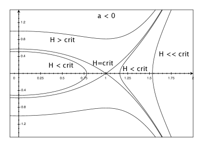
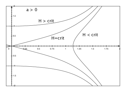
  Figure 3.1: Typical level curves of $H$ when $\beta>0$, ${\tilde{\sigma}}^{2}=0$

• $\beta>0$ and ${\tilde{\sigma}}\neq 0$: now $f$ decreases monotonically from $+\infty$ to $-\infty$, so there is a unique positive solution ${\tilde{\phi}}_{0}$ to (3.2) for any value of $a$; this is always an unstable critical point. Referring to the plot on the left in Figure 3.2, in the subcritical energy levels $H<\mbox{crit}$, ${\tilde{\phi}}$ either tends to infinity in both directions or tends to zero in both directions. In the supercritical energy levels, ${\tilde{\phi}}$ tends to $0$ in one direction and to infinity in the other. The nonconstant solutions at the critical level are asymptotic to the critical point $({\tilde{\phi}}_{0},0)$ at one end, while ${\tilde{\phi}}$ tends to either $0$ or infinity at the other.

• $\beta=0$ and ${\tilde{\sigma}}^{2}=0$; excluding the trivial case $a=0$, we see that when $a<0$ solution curves are all halves of ellipses which reach the line ${\tilde{\phi}}=0$ in finite time (this is the heavier curve in the right plot of Figure 3.2). When $a>0$, solution curves are hyperbolae for which ${\tilde{\phi}}$ is unbounded in either both directions, or else in only one direction and reach ${\tilde{\phi}}=0$ in finite time in the other; the exceptions are the curves at critical energy which exist for all time and lie along rays, tending toward the origin in one direction and to infinity in the other.

  

  

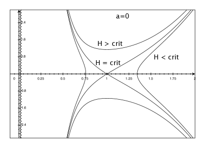
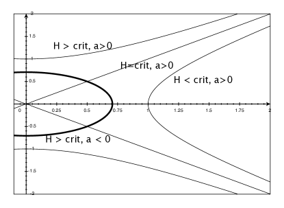
  Figure 3.2: Typical level curves of $H$ when $\beta,{\tilde{\sigma}}^{2}>0$ ($a=0$), and when $\beta={\tilde{\sigma}}^{2}=0$ for $a\neq 0$; $a>0$ corresponds to the heavier curve

• $\beta=0$ and ${\tilde{\sigma}}^{2}>0$: because ${\tilde{\sigma}}^{2}$ is nonzero, the solution curves remain in the open right halfplane for all time. Since the function $f$ decreases monotonically from $+\infty$ to $0$, there is a critical point only when $a>0$, and this is unstable, see the left plot of Figure 3.3. All solution curves have ${\tilde{\phi}}$ either unbounded or tending to zero in one or both directions. When $a\geq 0$, there is no critical point and, as in the right on Figure 3.3, all solution curves have ${\tilde{\phi}}\to 0$ both as $t\to\pm\infty$.

  

  

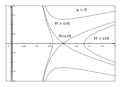
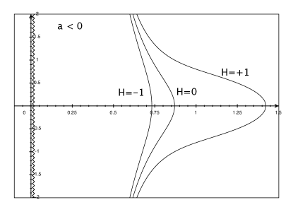
  Figure 3.3: Typical level curves of $H$ when $\beta=0$, ${\tilde{\sigma}}^{2}>0$, $a\neq 0$

• $\beta<0$ and ${\tilde{\sigma}}^{2}=0$: there is a critical point at $(0,0)$, and another at some point $({\tilde{\phi}}_{0},0)$ when $a>0$, see the left plot of Figure 3.4. When $a>0$, there is a homoclinic orbit connecting $(0,0)$ to itself in infinite time in both directions. The supercritical orbits, which lie outside this, reach ${\tilde{\phi}}=0$ in finite time both forwards and backwards. The orbits with energy less than zero and greater than $H({\tilde{\phi}}_{0},0)$ are periodic (these are the Delaunay solutions). When $a\leq 0$, all solutions exist only on a finite time interval.

• $\beta<0$ and ${\tilde{\sigma}}^{2}>0$: in this case $f$ is convex, with a unique critical point ${\tilde{\phi}}_{0}$:

  $${\tilde{\phi}}_{\mathrm{crit}}=\left(\frac{{\tilde{\sigma}}^{2}(\gamma+1)}{-\beta(\alpha-1)}\right)^{\frac{1}{\alpha+\gamma}}=\left(-\frac{{\tilde{\sigma}}^{2}}{\beta}(n-1)\right)^{\frac{n-2}{4n}}.$$

  A further calculation shows that

  $$f({\tilde{\phi}}_{\mathrm{crit}})=(-\beta)^{\frac{n-1}{n}}{\tilde{\sigma}}^{\frac{2}{n}}(n-1)^{\frac{1-n}{n}}n=:a_{0}.$$ (3.3)

  If $a<a_{0}$, equation (3.2) has no solutions, and only one when $a=a_{0}$. In these cases, all solutions (except $({\tilde{\phi}},\tilde{\psi})\equiv({\tilde{\phi}}_{0},0)$) have ${\tilde{\phi}}\to 0$ both as $t\to\pm\infty$. When $a>a_{0}$ there are two critical points, $(\phi_{0}^{\pm},0)$, see the right plot of Figure 3.4, with $0<{\tilde{\phi}}_{0}^{-}<{\tilde{\phi}}_{0}^{+}$ and $H({\tilde{\phi}}_{0}^{-})<H({\tilde{\phi}}_{0}^{+})$. There is a homoclinic orbit connecting $({\tilde{\phi}}_{0}^{-},0)$ to itself and defined for all $x\in\mathbb{R}$. Noncritical solution curves inside this orbit are periodic, and we call these the constraint Delaunay solutions. Solution curves outside the closure of this homoclinic orbit have ${\tilde{\phi}}\to 0$ either as $x\to\infty$ or $-\infty$ or both.

  

  

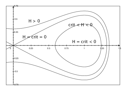
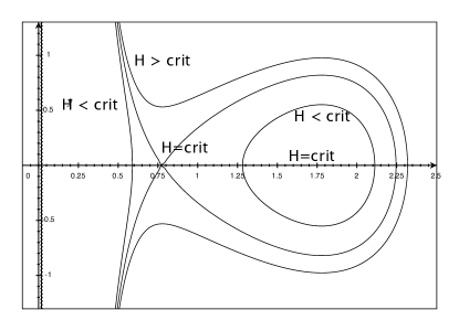
  Figure 3.4: Typical level sets of $H$ which include periodic orbits when $\beta<0$, ${\tilde{\sigma}}^{2}=0$ (left) and ${\tilde{\sigma}}^{2}>0$ (right); in the central enclosed regions in each figure, H=crit denotes the stationary point $({\tilde{\phi}}_{0},0)$.

To summarize, the only cases where there exist solutions for which ${\tilde{\phi}}$ remains bounded and uniformly positive for all $x$ are v) and vi), and in these two situations, the relevant solutions are either constant or else periodic. It is worth emphasizing that the minimum ‘necksize’ for the family of constraint Delaunay solutions in case vi) is strictly positive.

4 Manifolds with ends of cylindrical type

In this section we consider complete manifolds $(M,{\tilde{g}})$ which have a finite number of ends, each of cylindrical type. Thus each end $E_{\ell}$ of $M$ is identified with the product $\mathbb{R}^{+}\times N^{n-1}_{\ell}$, where $N_{\ell}$ is compact. In the most general scenario, the metric ${\tilde{g}}$ satisfies

$$c_{1}(dx^{2}+{\mathring{g}}_{\ell})\leq\left.{\tilde{g}}\right|_{E_{\ell}}\leq c_{2}(dx^{2}+{\mathring{g}}_{\ell})$$ (4.1)

for some positive constants $c_{1},c_{2}$ and fixed Riemannian metric ${\mathring{g}}_{\ell}$ on $N_{\ell}$. We are specifically interested in the cases when ${\tilde{g}}$ on each end is conformal to a metric which is either asymptotically cylindrical or asymptotically periodic, but the more general condition (4.1) will be allowed in some of our results. To set notation, we say that ${\tilde{g}}$ is asymptotically conformally cylindrical on the end $E_{\ell}$ if ${\tilde{g}}=w^{\frac{4}{n-2}}\check{g}$ there, where

$$\check{g}=dx^{2}+{\mathring{g}}_{\ell}+\mathcal{O}(e^{-\nu x}),$$

for some metric ${\mathring{g}}$ on $N_{\ell}$; ${\tilde{g}}$ is called asymptotically conformally periodic if $\check{g}$ is asymptotic at the same exponential rate to a metric ${\mathring{g}}$ on $\mathbb{R}\times N_{\ell}$ which is periodic in $x$ with period $T$. For convenience we often drop the index $\ell$ when the argument being made does not specifically address issues related to the presence of more than one end.

We also suppose that the functions $\beta$ and ${\tilde{\sigma}}^{2}$ converge to functions ${\mathring{\beta}}$ and ${\mathring{{\tilde{\sigma}}}}^{2}$ which are either independent of $x$ (in the conformally asymptotically cylindrical case) or else periodic with period $T$. Finally, we assume in both cases that the conformal factor $w$ converges to a function ${\mathring{w}}$, which is a smooth positive function on $N$. In all cases, convergence is at the rate $e^{-\nu x}$. While the methods here do not require much differentiability, we do need to assume that $\tilde{R}\to{\mathring{\tilde{R}}}$ in those results which assert existence of limits of the solution.

We shall construct solutions ${\tilde{\phi}}$ to the Lichnerowicz equation under various hypotheses. There is a preliminary very general result which assumes only that $\tilde{R}$ is negative and bounded away from $0$ far out in each end, but which requires almost nothing else about the structure of ${\tilde{g}}$ except that it is of cylindrical type. The rest of the results here assume some form of either of the conditions $\tilde{R}\leq-c$ or $\tilde{R}\geq 0$. To obtain solutions which have good asymptotic behavior, one needs to make more hypotheses than just cylindrical boundedness, and we prove such results in the asymptotically conformally cylindrical and periodic settings. If the putative solution ${\tilde{\phi}}$ converges to a limit ${\mathring{\phi}}$ (which is either a function on $N$ or else periodic on $\mathbb{R}\times N$), then ${\mathring{\phi}}$ must be a solution of the reduced Lichnerowicz equation

$$\Delta_{\mathring{g}}{\mathring{\phi}}-c(n){\mathring{\tilde{R}}}{\mathring{\phi}}={\mathring{\beta}}{\mathring{\phi}}^{\alpha}-{\mathring{{\tilde{\sigma}}}}^{2}{\mathring{\phi}}^{-\gamma}.$$ (4.2)

In the asymptotically periodic case, when ${\mathring{\phi}}$ is a function on $N$, this is not the Lichnerowicz equation on $N$, since the constants $c(n)$, $\alpha$ and $\gamma$ are for an $n$-dimensional manifold rather than an $(n-1)$-dimensional one. On the other hand, in the asymptotically periodic case this is the standard Lichnerowicz equation on the $n$-dimensional manifold $S^{1}\times N$. In any case, as part of the work ahead, we must prove existence of solutions to (4.2).

In several places below we shall use the Yamabe invariant of the conformal class $[{\tilde{g}}]$ on $M$. This is the value

$$Y(M,[{\tilde{g}}])= \inf_{u\in\mathcal{C}_{0}^{\infty}\atop{\ 0\leq u\not\equiv 0}}Q_{{\tilde{g}}}(u),$$ (4.3)

$$\mbox{where}\ Q_{{\tilde{g}}}(u)=\frac{\frac{1}{2}\int_{M}(|\nabla u|^{2}+c(n)\tilde{R}u^{2})}{\big{(}\int_{M}u^{\frac{2n}{n-2}}\big{)}^{\frac{n-2}{n}}}.$$

If $K$ is a compact domain in $M$ with smooth boundary, then $Y(K,[{\tilde{g}}])$ denotes the infimum of the same quantity amongst smooth nonnegative functions with support in $K$. We recall the well-known

Lemma 4.1.

Let $\lambda_{0}$ denote the lowest eigenvalue of $-L_{{\tilde{g}}}$ on $K$ with Dirichlet boundary conditions. Then $\lambda_{0}\neq 0$ if and only if $Y(K,[{\tilde{g}}])\neq 0$, and if this is the case, then the signs of $\lambda_{0}$ and $Y(K,[{\tilde{g}}])$ are the same.

Proof.

Let $\mathcal{R}_{{\tilde{g}}}$ denote the Rayleigh quotient for $-L_{{\tilde{g}}}$,

$$\mathcal{R}_{{\tilde{g}}}(v)=\frac{\frac{1}{2}\int_{K}(|\nabla v|^{2}+c(n)\tilde{R}v^{2})}{\int_{K}v^{2}}.$$ (4.4)

Since

$$\mathcal{R}_{{\tilde{g}}}(v)\int_{K}v^{2}=Q_{{\tilde{g}}}(v)\big{(}\int_{K}v^{\frac{2n}{n-2}}\big{)}^{\frac{n-2}{n}},$$ (4.5)

we see that $Q_{{\tilde{g}}}(v)$ and $\mathcal{R}_{{\tilde{g}}}(v)$ have the same sign for any $v$. From this it follows directly that $\lambda_{0}<0$ if and only if $Y(K,[{\tilde{g}}])<0$.

Thus we may now assume that $\lambda_{0}\geq 0$ and $Y(K,[{\tilde{g}}])\geq 0$, and it remains to show that either both of these quantities vanish, or neither of them do.

Applying Hölder’s inequality to (4.5) and using that $\mathcal{R}_{{\tilde{g}}}(v)\geq 0$ shows that $Q_{{\tilde{g}}}(v)\leq C\mathcal{R}_{{\tilde{g}}}(v)$ for some constant $C$ independent of $v$, hence if $\lambda_{0}=0$ then $Y(K,[{\tilde{g}}])=0$.

For the converse, recall the Sobolev inequality on $K$, which states that

$$\big{(}\int v^{2n/(n-2)}\big{)}^{(n-2)/n}\leq A\int|\nabla v|^{2}+B\int v^{2}\;,$$

for some constants $A$ and $B$. Rewrite the right side as

$$2A\big{(}\frac{1}{2}\int|\nabla v|^{2}+c(n)\tilde{R}v^{2})+\int(B-Ac(n)\tilde{R})v^{2}\\ \leq A^{\prime}\big{(}\frac{1}{2}\int|\nabla v|^{2}+c(n)\tilde{R}v^{2})+B^{\prime}\int v^{2}\;,$$

for some other constants $A^{\prime},B^{\prime}>0$. Dividing by $\int v^{2}$ and using that $Q_{{\tilde{g}}}(v),\mathcal{R}_{{\tilde{g}}}(v)\geq 0$ for all $v$, we obtain

$$\mathcal{R}_{{\tilde{g}}}(v)\leq Q_{{\tilde{g}}}(v)(A^{\prime}\mathcal{R}_{\tilde{g}}(v)+B^{\prime})\Rightarrow\mathcal{R}_{{\tilde{g}}}(v)\leq C^{\prime}Q_{{\tilde{g}}}(v)$$ (4.6)

for any $v\not\equiv 0$. This shows that if $Y(K,[{\tilde{g}}])=0$ then $\lambda_{0}=0$. This proves all the assertions in the lemma.

In what follows we will assume that $\tilde{R}$ remains bounded away from zero outside a compact set, or has constant sign everywhere, which is certainly restrictive. There are many cases of interest where this fails and the limiting scalar curvature ${\mathring{R}}$ changes sign. As already mentioned, those cases are not discussed here since they require fairly different techniques.

4.1 $\tilde{R}<0$ outside of a compact set

We begin with a general existence theorem assuming only that the scalar curvature $\tilde{R}$ is negative outside of a compact set. In this section we are mainly interested in complete manifolds with all ends of cylindrical type, but neither of these conditions is assumed in our next result:

Proposition 4.2.

Let $(M,{\tilde{g}})$ contain at least one cylindrical end. Suppose that there exist constants $c,C>0$ and a compact set $K$ such that

$$c\leq\beta\leq C\;,\quad-C\leq\tilde{R}\big{|}_{M\setminus K}\leq-c\;.$$ (4.7)

(No bound on ${\tilde{\sigma}}^{2}$ is required.) Then there exists a solution of the Lichnerowicz equation. The conformally rescaled metric is complete if ${\tilde{g}}$ is, and any end of cylindrical type remains cylindrical.

Proof.

We begin by using a result of Aviles and McOwen [4, Thm. A] that, given the hypotheses here, there exists a conformal deformation $\hat{g}=u^{\frac{4}{n-2}}{\tilde{g}}$ such that $\hat{R}\leq-c<0$ everywhere. Since the first paragraph (p. 230 in [4]) of their proof is not clear to us, we provide an alternative argument for that step of their proof.

It is not hard to see, by the assumption on the strict negativity of $\tilde{R}$ far out on the cylindrical end in particular, that we have $Y(K,[{\tilde{g}}])<0$. By Lemma 4.1, we must also have $\lambda_{0}<0$, where $\lambda_{0}$ is the lowest eigenvalue of $-L_{{\tilde{g}}}$ on $K$. If $u_{0}$ is the corresponding eigenfunction, then $L_{{\tilde{g}}}u_{0}=-\lambda_{0}u_{0}$, and this is strictly positive in the interior of $K$. Choose a large constant $A$ so that $Au_{0}>1$ in some slightly smaller compact set $K^{\prime}$ in the interior of $K$ but $Au_{0}<1$ near $\partial K$. Then set $u=\max\{Au_{0},1\}$ in $K$ and $u=1$ outside of $K$. Thus $L_{{\tilde{g}}}u\geq c>0$ weakly everywhere. Since $u$ is smooth away from the hypersurface $H$ where $Au_{0}=1$ (and by changing $A$ slightly we can always assume that $H$ is a smooth submanifold), it is not hard to see that this inequality is true in a distributional sense as well. Hence we can choose a mollification $\tilde{u}$ of $u$ which is smooth and satisfies $L_{{\tilde{g}}}\tilde{u}\geq c/2$ everywhere. Thus if $\hat{g}=\tilde{u}^{\frac{4}{n-2}}{\tilde{g}}$, then

$${\hat{R}}=-\frac{1}{c(n)}\tilde{u}^{-\alpha}L_{{\tilde{g}}}\tilde{u}$$

is everywhere negative and bounded between two negative constants.

We replace ${\tilde{g}}$ by the metric ${\hat{g}}$ and rename it ${\tilde{g}}$ again; we can thus assume that (4.7) holds with $K=\emptyset$.

With this reduction, we can immediately find a solution to the Lichnerowicz equation. Indeed, the bounds (4.7) imply that the constant function $\eta$ is a subsolution and $1/\eta$ is a supersolution when $0<\eta\ll 1$. The result now follows from Proposition A.4 in Appendix A.

If we drop the hypothesis on the lower bound $\tilde{R}\geq-C$, then we can proceed as in the later part of the proof of [4, Theorem A] to find a conformal factor $u$ which is bounded away from $0$ but not necessarily bounded above, so that the corresponding metric is complete, but does not necessarily have cylindrically bounded ends. It is probable that one can go on from this to find a solution of the Lichnerowicz equation. This certainly requires more work and we did not attempt it.

Proposition 4.2 is satisfactory in its generality, but has the defect that it gives very little information about the behavior of solutions far out in the ends. For metrics which are asymptotically cylindrical or asymptotically periodic, we can say much more. We take this up in the next two subsections.

4.1.1 Conformally asymptotically cylindrical ends

Let $(M,{\tilde{g}})$ be a complete manifold with conformally asymptotically cylindrical ends. Thus, as in the beginning of this section, ${\tilde{g}}=w^{\frac{4}{n-2}}g$, and all quantities considered here decay to asymptotic limits, which are functions or metrics on $N$, at the rate $e^{-\nu x}$ along with at least two derivatives. We assume also that in each end,

$${\mathring{\tilde{R}}}\leq-c\ \mbox{and}\ \beta\geq c\ \mbox{for some $c>0$}.$$

We now sharpen Proposition 4.2 in the sense that if we select any positive solution ${\mathring{\phi}}$ for the reduced Lichnerowicz equation (4.2) on each end, then there exists a solution ${\tilde{\phi}}$ which converges to ${\mathring{\phi}}$ at infinity. Hence even if we start with an asymptotically cylindrical metric, the solution metric is conformally asymptotically cylindrical. (Note too that there are many natural example of initial data sets with conformally asymptotically cylindrical ends, for example appropriate slices of the extremal Kerr metrics near their event horizon, see Appendix B.)

The existence of a unique limit function ${\mathring{\phi}}$ which solves (4.2) on each asymptotic cross-section $N^{n-1}$ is straightforward: with our hypotheses on ${\mathring{R}}$ and $\beta$, the constants $\eta$ and $1/\eta$, with $\eta$ sufficiently large, are sub- and supersolutions of (4.2), and uniqueness follows from the maximum principle.

Choose a smooth positive function $\phi$ which converges (at the rate $e^{-\nu x})$) to the limit function ${\mathring{\phi}}$ on each end. We shall look for solutions in the form $\phi(1+u)$ where $u\to 0$ at infinity. As in §2, we use the conformal transformation properties of the Lichnerowicz equation to write the equation as follows. Setting ${\hat{g}}=\phi^{\frac{4}{n-2}}{\tilde{g}}$, then

$$L_{\hat{g}}(1+u)=\beta(1+u)^{\alpha}-{\hat{\sigma}}^{2}(1+u)^{-\gamma},\ \mbox{where}\ {\hat{\sigma}}^{2}={\tilde{\sigma}}^{2}\phi^{-\frac{4n}{n-2}}.$$ (4.8)

Taking the limit of the conformal transformation rule $L_{{\tilde{g}}}\phi=\phi^{\alpha}L_{{\hat{g}}}1$ as $x\to\infty$ gives

$$(\Delta_{{\mathring{{\tilde{g}}}}}-c(n){\mathring{\tilde{R}}}){\mathring{\phi}}={\mathring{\phi}}^{\alpha}(-c(n){\mathring{{\hat{R}}}}),$$

and combining this with (4.2) for ${\mathring{\phi}}$ results in

$$\beta{\mathring{\phi}}^{\alpha}-{\mathring{{\tilde{\sigma}}}}^{2}{\mathring{\phi}}^{-\gamma}={\mathring{\phi}}^{\alpha}(-c(n){\mathring{{\hat{R}}}})\Longrightarrow c(n){\mathring{{\hat{R}}}}+{\mathring{\beta}}-{\mathring{{\hat{\sigma}}}}^{2}=0,$$

where ${\mathring{{\hat{\sigma}}}}^{2}$ is the limit of ${\hat{\sigma}}^{2}$. (We use here that $\partial_{x}\phi,\partial_{x}^{2}\phi=o(1)$.) We conclude the decay rate

$$s:=c(n){\hat{R}}+\beta-{\hat{\sigma}}^{2}=\mathcal{O}(e^{-\nu x})\;.$$ (4.9)

In order to construct the desired supersolution in the asymptotic region, we rewrite (4.8) using this estimate, also subtracting $\beta\alpha u$ from each side. This yields

$$\big{(}\Delta_{{\hat{g}}}- ({\hat{\sigma}}^{2}+\frac{4}{n-1}\beta+\mathcal{O}(e^{-\nu x}))\big{)}u=$$ (4.10)

$$\beta\left((1+u)^{\alpha}-1-\alpha u\right)+{\hat{\sigma}}^{2}\left(1-(1+u)^{-\gamma}\right)+s\;.$$

For simplicity, denote by $h$ the term of order zero in the linear operator on the left, i.e.

$$h={\hat{\sigma}}^{2}+\frac{4}{n-2}\beta+\mathcal{O}(e^{-\nu x}).$$

Note that $h\geq c>0$ for $x$ sufficiently large.

The motivation for this rearrangement is that the function

$$r(u)=\beta\left((1+u)^{\alpha}-1-\alpha u\right)+{\hat{\sigma}}^{2}\left(1-(1+u)^{-\gamma}\right)$$

satisfies $r(0)=0$ and is positive for $u>0$, as can be seen directly by differentiating.

To continue, observe that given ${\varepsilon}>0$ satisfying $4\epsilon^{2}<c$, we can choose $X_{\varepsilon}$ sufficiently large that

$${\hat{\sigma}}^{2}+\frac{4}{n-1}\beta+\mathcal{O}(e^{-\nu x})\geq 4{\varepsilon}^{2}\ \ \mbox{for}\ x\geq X_{\varepsilon}.$$

Now, for any $0<\delta<{\varepsilon}$, $\Delta_{\tilde{g}}e^{-\delta x}\leq 2{\varepsilon}^{2}e^{-\delta x}$, also for $x\geq X_{\varepsilon}$, whence

$$\left(\Delta_{{\hat{g}}}-h\right)e^{-\delta x}\leq-2\epsilon^{2}e^{-\delta x}$$

in $[X_{\varepsilon},\infty)\times N$. Finally, assuming that $\delta<\nu$, choosing

$$\hat{C}\geq\frac{\|e^{\nu x}s\|_{L^{\infty}}}{2\epsilon^{2}}e^{(\delta-\nu)X_{\epsilon}}$$

and $x\geq X_{\varepsilon}$, and using the positivity of $r$, we obtain

$$\left(\Delta_{{\hat{g}}}-h\right)\hat{C}e^{-\delta x}\leq s\leq s+r(\hat{C}e^{-\delta x}).$$

Comparing with (4.10), this says simply that $1+\hat{C}e^{-\delta x}$ is a supersolution.

We now show that $1-\hat{C}e^{-\delta x}$ is a subsolution in the asymptotic region if $\delta$ is sufficiently small. Using (4.9), we first calculate that

$$\begin{split}(\Delta_{\hat{g}}-c(n){\hat{R}})(1-\hat{C}e^{-\delta x})=(\Delta_{\hat{g}}+\beta-{\hat{\sigma}}^{2}+s)(1-\hat{C}e^{-\delta x})\\ =\big{(}-\hat{C}\Delta_{\hat{g}}e^{-\delta x}+s(1-\hat{C}e^{-\delta x})\big{)}+\big{(}\beta-{\hat{\sigma}}^{2})(1-\hat{C}e^{-\delta x})\big{)}.\end{split}$$ (4.11)

Setting $y=1-\hat{C}e^{-\delta x}$, then $y<1$ for all $x\geq 0$ and $\hat{C}\geq 0$. Fixing $\mu\in(0,1)$, $\delta\in(0,\nu)$ and any $\hat{C}>0$, we can choose $X=X(\hat{C},\delta)$ so large that for all $x\geq X$, we have $y\in[\mu,1)$, and moreover

$$\frac{y-y^{\alpha}}{1-y}\geq\mu^{\prime}>0\;,$$

for some positive number $\mu^{\prime}$ which depends only on $\mu$ and $\alpha$. This follows directly from the fact that the function on the left has a continuous extension to the closed interval $[\mu,1]$ and is everywhere positive there. This gives

$$1-\hat{C}e^{-\delta x}\geq\mu^{\prime}\hat{C}e^{-\delta x}+(1-\hat{C}e^{-\delta x})^{\alpha}.$$

It is also clear that

$$-{\hat{\sigma}}^{2}(1-\hat{C}e^{-\delta x})\geq-{\hat{\sigma}}^{2}(1-\hat{C}e^{-\delta x})^{-\gamma}.$$

Using these last two inequalities on the right side of (4.11), we see that

$$L_{\hat{g}}(1-\hat{C}e^{-\delta x})\geq\beta(1-\hat{C}e^{-\delta x})^{\alpha}-{\hat{\sigma}}^{2}(1-\hat{C}e^{-\delta x})^{-\gamma}+A,$$

where

$$A:=-\hat{C}\Delta_{\hat{g}}e^{-\delta x}+s(1-\hat{C}e^{-\delta x})+\beta\mu^{\prime}\hat{C}e^{-\delta x}.$$

The first term on the right here is $\mathcal{O}(\delta^{2}e^{-\delta x})$, while the second is bounded by $-\|e^{\nu x}s\|_{L^{\infty}}e^{-\nu x}$. Choosing $0<\delta\ll\nu$, we certainly have that $A\geq 0$ for $x$ large enough. This proves that $1-\hat{C}e^{-\delta x}$ is a subsolution sufficiently far out on the end.

We have now shown that, under the present hypotheses, we can construct sub- and supersolutions $1\pm\hat{C}e^{-\delta x}$ of (4.10) outside a sufficiently large compact set in $M$, with $\hat{C}$ as large as desired. To produce global barriers, we must argue a bit further. Recall that there is a conformally related metric $\bar{g}=\zeta^{\frac{4}{n-2}}{\tilde{g}}$, with $\zeta\to 1$ and $\partial\zeta,\partial^{2}\zeta$ going to zero exponentially fast, which has $\bar{R}\leq-c<0$ on all of $M$. So if we write the Lichnerowicz equation relative to this metric, then sufficiently small and large positive constants $\eta$ and $\eta^{-1}$ are sub- and supersolutions. This means that $\eta\zeta$ and $\eta^{-1}\zeta$ are global sub- and supersolutions for the equation relative to ${\hat{g}}$, and hence $\eta\phi\zeta$ and $\eta^{-1}\phi\zeta$ are global sub- and supersolutions for the equation relative to ${\tilde{g}}$.

All this leads us eventually to the global weak sub- and supersolutions

$$\max\{\phi(1-\hat{C}e^{-\delta x}),\eta\phi\zeta\}\ \mbox{and}\ \min\{\phi(1+\hat{C}e^{-\delta x}),\eta^{-1}\phi\zeta\}$$

for the original equation relative to ${\tilde{g}}$; the lower bound $\mu$ which appears in the argument above should be determined by $\mu:=\inf\eta\zeta>0$. Notice that these functions converge exponentially quickly to one another as $x\to\infty$, which controls as well the asymptotics of the solution which lies between them.

We have now proved:

Theorem 4.3.

Fix any number $c>0$ and suppose that $\beta\geq c$. Let ${\tilde{g}}$ be a metric with a finite number of asymptotically conformally cylindrical ends on $M^{n}$, $n\geq 3$, such that the limiting scalar curvature ${\mathring{\tilde{R}}}=\lim_{x\to\infty}\tilde{R}$ is strictly negative in each end. Assume also that ${\tilde{g}}$, $\tilde{R}$, ${\tilde{\sigma}}$ and $\beta$ all approach their limits on each end at the rate $e^{-\nu x}$. Then there exists a solution ${\tilde{\phi}}$ of the Lichnerowicz equation so that ${\tilde{\phi}}$ converges (at some exponential rate) to a limiting function ${\mathring{\phi}}$, which is a solution of (4.2). In particular, the solution metric ${\tilde{\phi}}^{\frac{4}{n-2}}{\tilde{g}}$ remains asymptotically conformally cylindrical.

4.1.2 Asymptotically periodic ends

As described at the beginning of this section, the metric ${\tilde{g}}$ is said to be conformally asymptotically periodic on an end $E_{\ell}$ if, on that end, ${\tilde{g}}=w^{\frac{4}{n-2}}g$ where $g$ differs from a metric $\check{g}$ which has period $T$ on $\mathbb{R}\times N$, where the difference is a tensor which has local Hölder norm decaying like $e^{-\nu x}$:

$$h:=g-\check{g}\ \,\mbox{satisfies}\ \|e^{\nu x}h\|_{2+\ell,\alpha}<\infty\ \mbox{for some}\ \nu>0\;.$$ (4.12)

The conformal factor $w$ is assumed to decay to a smooth periodic function at the same exponential rate. We also suppose that both $\sigma$ and $\beta$ decay like $e^{-\nu x}$ to functions $\check{\sigma}$ and $\check{\beta}$ which both have the same period $T$.

All such ends are cylindrically bounded, so Proposition 4.2 already guarantees the existence of solutions ${\tilde{\phi}}$ of the Lichnerowicz equation in this context if we assume that the scalar curvature is negative and bounded away from zero outside a compact set.

One special feature of this case is that we can exploit known results on compact manifolds. Thus suppose that ${\tilde{g}}$ is asymptotic to the periodic metric ${\check{g}}$. This induces a metric, which we give the same name, on $S^{1}_{T}\times N$ (here $S^{1}_{T}=\mathbb{R}/T\mathbb{Z}$). We can invoke the complete existence theory for the Yamabe problem on compact manifolds to choose a smooth positive conformal factor $\lambda$ on $S^{1}\times N$ such that $\lambda^{\frac{4}{n-2}}{\check{g}}$ has constant scalar curvature. This metric lifts to a periodic metric on $\mathbb{R}\times N$, and we can obviously replace ${\check{g}}$ by this new conformally related metric so as to assume that ${\tilde{g}}\sim\check{w}^{\frac{4}{n-2}}{\check{g}}$ where ${\check{g}}$ has constant scalar curvature. Note that even if ${\check{g}}$ is asymptotically cylindrical, i.e. ${\check{g}}=dx^{2}+{\mathring{g}}$, the modified metric may be only asymptotically periodic. The constraint Delaunay metrics in §3 are an example of this.

We now show that if the ends of $(M,{\tilde{g}})$ are all asymptotically conformally periodic, then there is a solution of the Lichnerowicz equation which has the same structure. To prove this, let ${\check{\phi}}\in\mathcal{C}^{2,\alpha}(S^{1}\times N)$ be the (strictly positive) solution of the limiting equation

$$L_{{\check{g}}}{\check{\phi}}=-\check{\sigma}^{2}{\check{\phi}}^{-\gamma}+\check{\beta}{\check{\phi}}^{\alpha}.$$ (4.13)

Assuming that $\check{R}\leq-c<0$, existence is easy: the subsolution is a small positive constant $\eta$ and the supersolution is a large positive constant $\eta^{-1}$.

Modifying the metric as above, we now search for solutions of the form ${\tilde{\phi}}=\phi+\psi$, where $\psi$ decays like $e^{-\nu x}$. It is then possible to follow the steps in the argument of § 4.1.1 almost exactly. This leads to the

Theorem 4.4.

Suppose that $\beta\geq c>0$, and let ${\tilde{g}}$ be a metric with a finite number of conformally asymptotically periodic ends on $M^{n}$, $n\geq 3$. Assume that $\tilde{R}\leq-c<0$ outside a compact set. Then there exists a solution ${\tilde{\phi}}$ of the Lichnerowicz equation so that each end remains asymptotically conformally periodic.

There is an obvious extension of Theorems 4.3 and 4.4 which allows $(M,{\tilde{g}})$ to have ends of both types. We leave details to the reader.

4.2 $\tilde{R}\geq 0$

We now consider metrics on a manifold with a finite number of conformally asymptotically cylindrical or periodic ends, assuming that $\tilde{R}$ enjoys certain positivity properties.

4.2.1 Yamabe positivity

We start with a discussion of the Yamabe invariant in the present context. The results here are only intended to provide an alternative perspective to the results of §4.2.2, and the analysis and results there are independent of the ones here.

Our initial result corresponds to the first step in the proof of Proposition 4.2. In that setting, if $\tilde{R}\leq-c<0$ outside a compact set, then without any further conditions it is possible to make an initial conformal change to arrange that $\tilde{R}\leq-c<0$ on all of $M$. The analogue of this result when $\tilde{R}\geq 0$ requires an extra hypothesis on the Yamabe invariant, as defined in (4.3).

It is well known that if $M$ is compact, then $-\infty<Y(M,[{\tilde{g}}])\leq Y(S^{n})$, and that the infimum of the functional $Q_{{\tilde{g}}}$ is always realized. For manifolds with exactly cylindrical ends, a parallel though somewhat less complete theory is developed in [1]. Suppose that the ends are modelled on the products $(\mathbb{R}^{+}\times N_{\ell},dx^{2}+{\mathring{g}}_{\ell})$. As before, we assume for simplicity that there is only one end and drop the subscript $\ell$. Although [1] assumes that the restriction of ${\tilde{g}}$ on the end is exactly of product type, it is not hard to extend their results to the case of asymptotically cylindrical metrics, see [2]. Furthermore, if ${\tilde{g}}$ is conformally asymptotically cylindrical, so ${\tilde{g}}=w^{4/(n-2)}\check{g}$, where $\check{g}$ is asymptotically cylindrical, then it is obvious that $Y(M,[{\tilde{g}}])=Y(M,[\check{g}])$. Thus we may talk about the Yamabe invariant in this slightly more general setting.

One of the key points in [1] is that $Y(M,[{\tilde{g}}])$ is regulated by the lowest eigenvalue $\mu_{0}$ of the operator

$$-\mathcal{L}_{{\mathring{g}}}:=-\Delta_{{\mathring{g}}}+c(n){\mathring{R}},$$ (4.14)

which we have already encountered as the linear part of the reduced Lichnerowicz operator (4.2). (Just as for that operator, this is not the conformal Laplacian on $N$ because the constant $c(n)$ is appropriate for an $n$-dimensional manifold, not an $(n-1)$-dimensional one.) The first main result [1, Lemma 2.9] is that $\mu_{0}\geq 0$ if and only if $Y(M,[{\tilde{g}}])>-\infty$. It is not hard to see that

$$Y(M,[{\tilde{g}}])\leq Y(\mathbb{R}\times N,[dx^{2}+{\mathring{g}}])\leq Y(S^{n}),$$ (4.15)

with the second equality sharp except when $(M,{\tilde{g}})$ is conformal to the sphere, with its standard metric, punctured at a finite number of points. If $Y(M,[{\tilde{g}}])<Y(\mathbb{R}\times N,[dt^{2}+{\mathring{g}}])$ and $\mu_{0}>0$, then there exists a metric in $[{\tilde{g}}]$ which minimizes the Yamabe functional, but this metric is incomplete, with isolated conic singularities and the minimizing function $u$ decays exponentially along the ends. (If $\mu_{0}=0$ the existence theory is more complicated, and the solutions when they exist are complete but of cusp type.) The paper [2] contains a substantial generalization of their result and a closer investigation of the asymptotics of the solution, even in the cylindrical setting.

Before stating our first result, we recall an alternate characterization of the positivity of the Yamabe invariant which is needed in the argument.

Lemma 4.5.

Let $(M,{\tilde{g}})$ be a complete manifold with ends which are conformally asymptotically cylindrical or periodic. Then the condition $Y(M,[{\tilde{g}}])>0$ is equivalent to the pair of conditions

$$\mathrm{i)} L^{2} -L_{{\tilde{g}}} [0,\infty)$$ the spectrum of lies in , and (4.16)

$$\mathrm{ii)} 0 -L_{{\tilde{g}}}$$   does not lie in the point spectrum of . (4.17)

Before starting the proof, we remark that unlike Lemma 4.1, where we only considered the signs of these invariants on a compact manifold with boundary, here we consider their behaviour on the noncompact manifold $M$.

Proof.

Denote by $\lambda_{0}(K)$ the lowest eigenvalue of $-L_{{\tilde{g}}}$ with Dirichlet boundary conditions on any smoothly bounded compact subdomain of $M$, and $Y(K,[{\tilde{g}}])$ the Yamabe invariant of any such subdomain. By Lemma 4.1, these have the same sign for any $K$. By (strict) domain monotonicity, if $\lambda_{0}(M)\geq 0$ then $\lambda_{0}(K)>0$ for any $K$, hence $Y(K,[{\tilde{g}}])>0$ and finally $Y(M,[{\tilde{g}}])\geq 0$. Similar reasoning shows that if $Y(M,[{\tilde{g}}])>0$ then $\lambda_{0}(M)\geq 0$.

It suffices now to prove that $0$ is an $L^{2}$ eigenvalue if and only if $Y(M,[{\tilde{g}}])=0$. Suppose first that $0$ is an $L^{2}$ eigenvalue, and let $u_{0}$ be the corresponding eigenfunction. Elliptic regularity implies that $u_{0}$ is as differentiable as the metric allows, and completeness of $M$ together with the usual sequence of cutoffs shows that $u_{0}\in H^{1}(M)$, with $u_{0}>0$. Since the ends of $(M,{\tilde{g}})$ are cylindrically bounded, we claim that $(M,{\tilde{g}})$ admits a Sobolev inequality (we substantiate this momentarily), and hence $u_{0}\in L^{2n/(n-2)}$ as well. It is then straightforward to check that cutting off $u_{0}$ to be supported in larger and larger sets gives a minimizing sequence for $Q_{{\tilde{g}}}$, so that $Y(M,[{\tilde{g}}])=0$. In fact, $u_{0}$ itself is a minimizer for this functional and $Q_{{\tilde{g}}}(u_{0})=0$.

Regarding the claim about the existence of a Sobolev inequality, we recall the following standard facts (discussed in more detail in [2]). First, the existence of a Sobolev inequality is a quasi-isometry invariant, so we may as well assume that $(M,{\tilde{g}})$ has exact cylindrical ends. Next, such an inequality is localizable, so it is enough to show that any cylinder $\mathbb{R}\times N$, where $N$ is compact, admits a Sobolev inequality. Finally, if a Sobolev inequality holds for $N_{1}$ and $N_{2}$, then it holds for the Riemannian product $N_{1}\times N_{2}$. Thus since any compact manifold $N$ admits a Sobolev inequality, as does the real line, we see that the same is true for the cylinder, and hence the manifold $M$.

Suppose conversely that $Y(M,[{\tilde{g}}])=0$. We now quote [2, Proposition 1.1], which guarantees in this setting that $Y(\mathbb{R}\times N,[dx^{2}+{\mathring{g}}])>0$ because $(M,[{\tilde{g}}])$ admits a Sobolev inequality. But now we may apply [1, Theorem A], which asserts that since $Y(M,[{\tilde{g}}])<Y(\mathbb{R}\times N,[dx^{2}+{\mathring{g}}])$, there exists a minimizer $u$ for $Q_{{\tilde{g}}}$, so that $Q_{{\tilde{g}}}(u)=0$. Theorem B of that same paper asserts that $u$ decays exponentially, and thus lies in $L^{2}$. Since the Euler-Lagrange equation for $Q_{{\tilde{g}}}$ for this function $u$ is simply $-L_{{\tilde{g}}}u=0$, we see that $0$ is an $L^{2}$ eigenvalue.

Proposition 4.6.

Suppose that $(M,{\tilde{g}})$ has conformally asymptotically cylindrical or periodic ends, and that $Y(M,[{\tilde{g}}])>0$. Then there exists $u\in\mathcal{C}^{\infty}(M)$ with $u>0$ on all of $M$ and $u\to u_{0}>0$ as $x\to\infty$, where $u_{0}\in\mathcal{C}^{\infty}(N)$ in the cylindrical case and $u_{0}\in\mathcal{C}^{\infty}(S^{1}\times N)$ in the periodic case, such that $\check{g}=u^{4/(n-2)}{\tilde{g}}$ has $\check{R}>0$ everywhere.

Proof.

We proceed by modifying the metric in two steps: in the first, we change conformally to a metric which has strictly positive scalar curvature outside a compact set, and in the second we arrange that the scalar curvature becomes positive everywhere. As noted earlier, we may as well replace the metric ${\tilde{g}}$ by the conformally related one $\check{g}$ which is asymptotic to $dx^{2}+{\mathring{g}}$ in the asymptotically cylindrical setting and to ${\mathring{g}}$ in the asymptotically periodic setting. We discuss the former case first.

For the first step, by our hypothesis and (4.15), we see that $Y(\mathbb{R}\times N,[dx^{2}+{\mathring{g}}])>0$. By [1, Lemma 2.9], this implies that $\mu_{0}>0$, where as above, $\mu_{0}$ is the lowest eigenvalue of $-\mathcal{L}_{{\mathring{g}}}$. Let $\psi_{0}$ be the ground state eigenfunction for $\mathcal{L}_{{\mathring{g}}}$, so that $\mathcal{L}_{{\mathring{g}}}\psi_{0}=-\mu_{0}\psi_{0}$ and $\psi_{0}>0$ on $N$.

Now choose a function $\psi$ which is strictly positive on all of $M$ and which equals $\psi_{0}$ far out on each end. Define $\overline{g}=\psi^{\frac{4}{n-2}}\check{g}$. Then

$$L_{\check{g}}\psi=-c(n)\overline{R}\psi^{\alpha}.$$

Comparing this with the fact that $L_{\check{g}}\psi\to\mathcal{L}_{{\mathring{g}}}\psi_{0}=-\mu_{0}\psi_{0}$ as $x\to\infty$, we see that $\overline{R}\geq c>0$ outside a compact set.

For simplicity, rename the new metric as ${\tilde{g}}$ again, so that we now prove our statement assuming that $\tilde{R}\geq c>0$ far out on the ends.

For the next step, choose a smooth function $f$ which equals $-c(n)\tilde{R}$ outside a large compact set and such that $f\leq-c<0$ everywhere. We claim that there is a unique bounded solution to the equation $L_{\tilde{g}}u=f$. Setting $u=1+v$, we can rewrite this equation as

$$L_{{\tilde{g}}}v=f+c(n)\tilde{R}:=\tilde{f}.$$

By construction $\tilde{f}$ is compactly supported.

We construct barrier functions for this equation. By Lemma 4.5, the spectrum of $-L_{{\tilde{g}}}$ is nonnegative and $0$ is not an $L^{2}$ eigenvalue. Since we have arranged that $\tilde{R}\geq c>0$ on the ends, the continuous spectrum of $-L_{{\tilde{g}}}$ must lie in a ray $[c^{\prime},\infty)$ for some $c^{\prime}>0$, hence the interval $(0,c^{\prime})$ contains only isolated $L^{2}$ eigenvalues of finite rank. Putting these facts together, we see that $0$ does not lie in the closure of the spectrum.

To proceed, assume first that the bottom of the spectrum of $-L_{{\tilde{g}}}$ is an isolated $L^{2}$ eigenvalue $\lambda_{0}>0$. Thus $\lambda_{0}$ is necessarily simple and there exists a strictly positive $L^{2}$ eigenfunction $\phi_{0}$ on $M$ such that $-L_{{\tilde{g}}}\phi_{0}=\lambda_{0}\phi_{0}$. Now, since $\tilde{f}$ is compactly supported and $\phi_{0}>0$ everywhere, we can choose $A\gg 0$ so that

$$L_{{\tilde{g}}}A\phi_{0}=-A\lambda_{0}\phi_{0}\leq\tilde{f},\quad\mbox{and}\quad L_{{\tilde{g}}}(-A\phi_{0})=A\lambda_{0}\phi_{0}\geq\tilde{f}.$$

By Proposition A.1 in Appendix A, this gives a solution $v$ to $L_{{\tilde{g}}}v=\tilde{f}$ with $-A\phi_{0}\leq v\leq A\phi_{0}$. Since ${\tilde{g}}$ is conformally asymptotically cylindrical or periodic, it is known that $\phi_{0}$ decays exponentially (see [2] for the cylindrical case and [42] for the periodic case).

If there is no $L^{2}$ eigenvalue below the continuous spectrum, we can still obtain sub- and supersolutions as follows. Fix any $0<\lambda<\inf\mbox{spec}\,(-L_{{\tilde{g}}})$. A theorem due to Sullivan [48, Theorem 2.1] gives the existence of a strictly positive function $\phi$ such that $L_{{\tilde{g}}}\phi=-\lambda\phi$. Strictly speaking, Sullivan’s theorem is only stated for the Laplace operator itself rather than for an operator of the form $\Delta_{{\tilde{g}}}-c(n)\tilde{R}$. However, inspection of the proof [48, p. 337] shows that the proof adapts immediately to this slightly more general setting since it relies only on the Harnack inequality, the existence of which for $L_{{\tilde{g}}}$ is classical [23].

Choose a large compact set $K\subset M$ so that $\tilde{R}\geq c>0$ outside $K$. Then $L_{{\tilde{g}}}e^{-\epsilon x}\leq-c^{\prime}e^{-\epsilon x}$ outside of $K$. Choose a slightly smaller compact set $K^{\prime}\subset K$ and a constant $\eta>0$ so that $\eta\phi>e^{-\epsilon x}$ on $\partial K^{\prime}$ but $\eta\phi<e^{-\epsilon x}$ on $\partial K$, and then define $\tilde{\phi}=\min\{\eta\phi,e^{-\epsilon x}\}$ in $K\setminus K^{\prime}$, $\tilde{\phi}=\eta\phi$ in $K^{\prime}$ and $\tilde{\phi}=e^{-\epsilon x}$ outside of $K$. This is the minimum of two supersolutions in the overlap region $K\setminus K^{\prime}$ and equal to a smooth supersolution outside of the overlap, so is a global weak supersolution (compare Appendix A). It is also strictly positive and uniformly bounded. Thus, as before, sufficiently large multiples of $-\tilde{\phi}$ and $\tilde{\phi}$ serve as barriers to find a solution $v$ which, as before, decays exponentially.

To conclude the argument, the function $u=1+v$ solves $L_{{\tilde{g}}}u=f<0$. We know that $u>0$ outside a large compact set. To show that $u>0$ everywhere, choose a smoothly bounded compact set $K$ so that $\tilde{R}>0$ outside $K$, and let $\lambda_{0}(K)$ be the lowest eigenvalue of $-L_{{\tilde{g}}}$ with Dirichlet boundary conditions on $K$. If $K$ is sufficiently large, $\lambda_{0}(K)>0$ and the associated eigenfunction $\phi_{0}$ is strictly positive. A brief calculation shows that

$$\Delta_{{\tilde{g}}}\frac{u}{\phi_{0}}+2\frac{\nabla\phi_{0}}{\phi_{0}}\cdot\nabla(\frac{u}{\phi_{0}})-\lambda_{0}(K)\frac{u}{\phi_{0}}=\frac{f}{\phi_{0}}<0\;.$$

This equation shows that $u/\phi_{0}$ cannot attain a nonpositive minimum at any point $q\in K$, and since $u/\phi_{0}\to+\infty$ at $\partial K$, we conclude that $u>0$ everywhere.

The modifications of this argument to the conformally asymptotically periodic setting are straightforward and left to the reader.

4.2.2 The Lichnerowicz equation

Let us now return to the main problem. We assume that $(M,{\tilde{g}})$ has conformally asymptotically cylindrical or periodic ends, and $0\leq\beta\leq C$. We also assume that one of the following two hypotheses holds:

• $Y(M,[{\tilde{g}}])>0$, so by Proposition 4.6, we may as well assume that $0<c\leq\tilde{R}\leq C$ on all of $M$, or

• $0\leq\tilde{R}\leq C$ on all of $M$ and $\tilde{R}+\beta\geq c>0$ outside some compact set.

We shall use an argument of Maxwell [38] (see [26] for a similar idea) which we explain first in the following setting. Let $h$, $a$, and $f$ be smooth functions on a compact Riemannian manifold $(N,{\mathring{g}})$, with $f\geq 0$, $a\geq 0$ and $f+h\geq c>0$. Consider the equation

$$\Delta_{{\mathring{g}}}u-hu=fu^{\alpha}-au^{-\gamma}$$ (4.18)

(the specific values of $\alpha>1$ and $\gamma>0$ are unimportant here). We also require that $a\not\equiv 0$.

By the strict positivity of $h+f$ (and the compactness of $N$), there exists a unique $u_{1}$ such that

$$\Delta_{\mathring{g}}u_{1}-(h+f)u_{1}=-a\;.$$ (4.19)

This function is strictly positive by the maximum principle. If $t>0$ is sufficiently small, then $u_{t}=tu_{1}$ is a subsolution of (4.18): indeed, $ta\leq at^{-\gamma}u^{-\gamma}_{1}$ and $ftu_{1}\geq ft^{\alpha}u^{\alpha}_{1}$ for $t\ll 1$, thus

$$\Delta_{\mathring{g}}u_{t}-hu_{t}=-ta+tu_{1}f\geq-at^{-\gamma}u^{-\gamma}_{1}+ft^{\alpha}u^{\alpha}_{1}\;.$$ (4.20)

On the other hand, a large positive constant provides a supersolution. Hence (4.18) has a solution.

In our particular setting, if ${\mathring{\beta}}\geq 0$, ${\mathring{\tilde{R}}}\geq 0$ and ${\mathring{\beta}}+{\mathring{\tilde{R}}}\geq c>0$, and in addition, ${\mathring{{\tilde{\sigma}}}}^{2}\not\equiv 0$, then we immediately obtain a solution ${\mathring{\phi}}$ of the limiting equation (4.2) by this argument.

Now we adapt this same construction to a manifold $(M,{\tilde{g}})$ with conformally asymptotically cylindrical ends. The analogue of (4.19) is now

$$\Delta_{\tilde{g}}u_{1}-(c(n)\tilde{R}+\beta)u_{1}=-{\tilde{\sigma}}^{2}\;.$$ (4.21)

We assume that $\tilde{R}$, $\beta$ and ${\tilde{\sigma}}^{2}$ converge to their asymptotic limits ${\mathring{\tilde{R}}}$, ${\mathring{\beta}}$ and ${\mathring{{\tilde{\sigma}}}}^{2}\not\equiv 0$ at an exponential rate $e^{-\nu x}$ in the sense that $\tilde{R}-{\mathring{\tilde{R}}}\in e^{-\nu x}\mathcal{C}^{0,\mu}(M)$ for some $\mu\in(0,1)$, and similarly for the other two functions. Here $\mathcal{C}^{0,\mu}(M)$ consists of all functions $u\in\mathcal{C}^{0,\mu}_{\mathrm{loc}}(M)$ such that

$$\sup_{X\geq 0}||u||_{0,\mu,[X,X+1]\times N}<\infty,$$

where $||\cdot||_{0,\mu,[X,X+1]\times N}$ denotes the Hölder norm on the finite cylindrical section where $X\leq x\leq X+1$.

As above, fix a solution ${\mathring{u}}$ of the limiting equation (4.2). In the asymptotically periodic case we make the obvious corresponding hypotheses, with ${\mathring{\tilde{R}}}$, ${\mathring{\beta}}$ and ${\mathring{{\tilde{\sigma}}}}^{2}$ periodic, all with the same period as the metric, and we can then choose a periodic solution ${\mathring{u}}$.

Choose a function ${\mathring{u}}_{1}$ which coincides with ${\mathring{u}}$ far out on each end. We seek a solution of (4.21) of the form $u_{1}={\mathring{u}}_{1}+v$. Thus $v$ must satisfy

$$\Delta_{\tilde{g}}v-(c(n)\tilde{R}+\beta)v=-{\tilde{\sigma}}^{2}-(\Delta_{\tilde{g}}{\mathring{u}}_{1}-(c(n)\tilde{R}+\beta){\mathring{u}}_{1})\;.$$ (4.22)

One readily checks that in either the asymptotically conformally cylindrical or periodic settings, the right-hand side lies in $e^{-\nu x}\mathcal{C}^{0,\mu}(M)$. Using the functions

$$\phi=\min\{1,Ae^{-\nu^{\prime}x}\}$$

and $-\phi$ as super- and subsolutions, where $0<\nu^{\prime}<\nu$ and $A\gg 0$, we obtain a bounded solution of this equation. Since $u_{1}={\mathring{u}}_{1}+v\to{\mathring{u}}>0$ as $x\to\infty$, it must be strictly positive outside a large compact set; the maximum principle applied to (4.21) gives $u_{1}\geq c>0$ everywhere.

Finally, the same calculation (4.20) shows that $u_{-}:=tu_{1}$ is a strictly positive subsolution of (4.21) when $0<t\ll 1$, while a large constant $u_{+}:=C$ provides a supersolution.

Calculations similar to those of Section 4.1.1 (in fact simpler because for $\tilde{R}\geq c>0$ no careful study of the right hand side is needed) show that ${\mathring{u}}\pm Ce^{-\delta x}$ are also sub- and supersolutions for a sufficiently small $\delta>0$. Hence

$${\tilde{\phi}}_{-}=\max({\mathring{u}}-Ce^{-\delta x},u_{-})\ \mbox{and}\ {\tilde{\phi}}_{+}=\min({\mathring{u}}+Ce^{-\delta x},u_{+})$$ (4.23)

are weak sub- and supersolutions of the Lichnerowicz equation.

Altogether, we have proved the

Theorem 4.7.

Let $(M,{\tilde{g}})$ have a finite number of conformally asymptotically cylindrical and periodic ends. Suppose that either of the hypotheses a) or b) above hold, and

$$\beta-{\mathring{\beta}}=\mathcal{O}(e^{-\nu x})\;,\qquad{\tilde{\sigma}}^{2}-{\mathring{{\tilde{\sigma}}}}^{2}=\mathcal{O}(e^{-\nu x})\;,\qquad{\mathring{{\tilde{\sigma}}}}^{2}\not\equiv 0\;,$$

for some functions ${\mathring{{\tilde{\sigma}}}}^{2}>0$, ${\mathring{\beta}}$ on $N$ in the asymptotically cylindrical ends, and for some functions ${\mathring{{\tilde{\sigma}}}}^{2}$, ${\mathring{\beta}}$ on $S^{1}\times N$ in the asymptotically periodic ends. Then there exists a solution ${\tilde{\phi}}$ of the Lichnerowicz equation so that each end of cylindrical type remains of the same type for the metric ${\tilde{\phi}}^{\frac{4}{n-2}}{\tilde{g}}$.

5 Manifolds with asymptotically hyperbolic and cylindrical ends

The constructions in Section 4.1 generalize immediately to manifolds which have a finite number of ends, some asymptotically hyperbolic, as defined in [3], and the others cylindrically bounded. The cylindrical ends are handled as in the Section 4.1, while the asymptotically hyperbolic ones are treated as in [3]. The reader should have no difficulties supplying the details to establish the following

Theorem 5.1.

Let $(M,{\tilde{g}})$ be a Riemannian manifold of dimension $n\geq 3$ with a finite number of conformally asymptotically cylindrical or periodic ends and a finite number of asymptotically hyperbolic ends. Suppose that $\beta\geq c>0$, and that in each asymptotically cylindrical end, the limiting scalar curvature ${\mathring{R}}$ is negative. We assume moreover that $\beta$ approaches a constant and ${\tilde{\sigma}}^{2}$ approaches zero in the asymptotically hyperbolic ends with the usual rates as in [3], and in addition that on each cylindrical end

$${\tilde{\sigma}}^{2}-{\mathring{{\tilde{\sigma}}}}^{2}=O(e^{-\epsilon x})\;,$$

for some bounded function ${\mathring{{\tilde{\sigma}}}}^{2}$ on $N$. Then there exists a solution ${\tilde{\phi}}$ of the Lichnerowicz equation so that in the conformally rescaled metric, each end has the same type as for ${\tilde{g}}$.

6 Manifolds with asymptotically flat and cylindrical ends, $\tilde{R}\geq 0$

We now extend the analysis of §4.2 and suppose that $(M,{\tilde{g}})$ is a complete manifold with a finite number of ends, each one either cylindrical with $\tilde{R}\geq 0$, or else asymptotically Euclidean or conical. As mentioned in the introduction, it is simpler to refer to this last case as only asymptotically Euclidean, the conical case being understood. We only consider the problem with

$$\Lambda=0,\;,$$

and assume that $\beta\geq 0$, with both $\beta$ and ${\tilde{\sigma}}^{2}$ tending to zero in the asymptotically Euclidean ends faster than $r^{-2-\epsilon}$ for some $\epsilon>0$. We also assume that ${\tilde{\sigma}}^{2}\to{\mathring{{\tilde{\sigma}}}}^{2}\not\equiv 0$ and $\beta\to{\mathring{\beta}}$ exponentially fast along each asymptotically conformally cylindrical (in which case ${\mathring{{\tilde{\sigma}}}}^{2}$ and ${\mathring{\beta}}$ are functions on $N$) or asymptotically periodic end (in which case ${\mathring{{\tilde{\sigma}}}}^{2}$ and ${\mathring{\beta}}$ are periodic on $\mathbb{R}\times N$, with the same period as the metric). Finally, we assume that sufficiently far out in the cylindrical ends the scalar curvature is bounded away from zero.

Special cases of the construction in this section have been considered in [15, 49, 17, 18]. The reader is referred to [10, 21, 11, 30] and references therein for more information on the constraint equations on asymptotically flat manifolds.

We start by arranging that ${\tilde{g}}$ has controlled curvature in the asymptotically Euclidean regions. For some constant $r_{0}\gg 0$ to be chosen below, let $\chi$ be a smooth nonnegative function which equals one for $r\geq r_{0}$ in the asymptotically Euclidean ends and vanishes for $r\leq r_{0}-1$ and elsewhere on $M$. Let $\mu\in\mathcal{C}^{\infty}$ be a small, nonnegative function with support in $\{r\leq 3r_{0}\}$ such that $\mu+\tilde{R}>0$ when $\{r\leq 2r_{0}\}$. Now, let $v$ be a solution of the equation

$$L_{{\tilde{g}}}v+\chi{\tilde{\sigma}}^{2}+\mu=0$$ (6.1)

such that $v\to 0$ on all the ends. We assume that on each such end

$${\tilde{\sigma}}^{2}\in\rho_{e}^{-\nu-2}{\cal C}^{0,\alpha}_{\tilde{g}}$$

for some $-\nu\in(2-n,0)$ and that

$${\tilde{\sigma}}^{2}-{\mathring{{\tilde{\sigma}}}}^{2}\in\rho_{c}^{-\nu}{\cal C}^{0,\alpha}\;,\quad{\mathring{{\tilde{\sigma}}}}^{2}\not\equiv 0$$

on each conformally asymptotically cylindrical end, with $\nu$ sufficiently small as determined by the dimension and by the asymptotic behavior of $\tilde{R}$ in the cylindrical ends. It is proved in Appendix A that with these decay conditions, and since $\tilde{R}\geq 0$, a solution $v$ exists.

It is straightforward from this method of proof that $v$ tends uniformly to zero as $r_{0}\nearrow\infty$ and $\mu$ is made smaller. Thus we may assume that

$$1+v\geq\frac{1}{2}\;.$$

The scalar curvature of the metric $\overline{g}=(1+v)^{\frac{4}{n-2}}{\tilde{g}}$ is equal to

$$\overline{R}=\frac{-L_{{\tilde{g}}}(1+v)}{c(n)(1+v)^{\frac{n+2}{n-2}}}=\frac{\tilde{R}}{(1+v)^{\frac{n+2}{n-2}}}+\frac{(\chi{\tilde{\sigma}}^{2}+\mu)}{c(n)(1+v)^{\frac{n+2}{n-2}}}\;.$$ (6.2)

From this we see that $\overline{R}>0$ everywhere and $\overline{R}\geq c{\tilde{\sigma}}^{2}$ for $r\geq r_{0}$ in the asymptotically Euclidean and conical regions. For simplicity, we write this new metric $\overline{g}$ as ${\tilde{g}}$ again.

We now adapt to this setting the construction of barrier functions from §4.2. The hypotheses in the cylindrical ends are identical to those in that section. Consider again the equation (4.21),

$$\Delta_{\tilde{g}}u_{1}-(h+f)u_{1}=-a\;.$$ (6.3)

In each asymptotically conformally cylindrical end we solve the limiting equation

$$\Delta_{\mathring{g}}{\mathring{u}}_{1}-(\,{\mathring{\!h}}+\mathring{f}){\mathring{u}}_{1}=-{\mathring{a}};$$ (6.4)

the function ${\mathring{u}}_{1}$ on $N$ is strictly positive by the maximum principle. Similarly, on each asymptotically periodic case we obtain a positive periodic solution ${\mathring{u}}_{1}$.

Now let ${\mathring{u}}$ denote any function on $M$ which coincides with ${\mathring{u}}_{1}$ far out in each cylindrical end and which equals one on each asymptotically Euclidean or conical end. We search for a solution $u_{1}$ of (6.3) by setting $u_{1}={\mathring{u}}+v$. The function $v$ must satisfy

$$(\Delta_{\tilde{g}}-(h+f))v=-a-(\Delta_{\tilde{g}}-(h+f)){\mathring{u}}\;.$$ (6.5)

This has suitable behavior in each asymptotic ends so that we may use the barrier functions described in Appendix A. We obtain a solution $v$ which satisfies $v\in e^{-\nu_{1}x}\mathcal{C}^{2,\alpha}(M)$ in the cylindrical ends, for some $\nu_{1}\in(0,\nu)$, and such that $v$ decays faster than $r^{-\epsilon}$ on the asymptotically Euclidean and conical ends.

The solution $u_{1}={\mathring{u}}+v$ of (4.21) tends to the strictly positive function ${\mathring{u}}$, hence $u_{1}$ must be strictly positive far out on the cylindrical ends. The maximum principle applied to (6.3) shows that $u_{1}\geq c>0$. The calculation (4.20) shows that $u_{-}:=tu_{1}$ is a strictly positive subsolution of (4.21) when $t>0$ is sufficiently small.

On the other hand, a large constant $u_{+}:=C$ provides a supersolution. This is clear for any domain $K$ in $M$ which does not intersect the asymptotically Euclidean or conical regions since the scalar curvature $\tilde{R}$ is strictly positive. On these other ends, we see that it is a supersolution using that $\tilde{R}\geq c{\tilde{\sigma}}^{2}$.

We now use the definition (4.23) in the cylindrical ends and

$${\tilde{\phi}}_{-}=\max(1-Cr^{-\delta},u_{-})\ \mbox{and}\ {\tilde{\phi}}_{+}=\min(1+Cr^{-\delta},u_{+})\;.$$ (6.6)

on the asymptotically Euclidean and conic ends, for $\delta>0$ sufficiently small.

All of this leads to the

Theorem 6.1.

Let $(M^{n},{\tilde{g}})$ be a complete Riemannian manifold, $n\geq 3$, with a finite number asymptotically Euclidean and conical ends and a finite number of conformally asymptotically cylindrical and periodic ends. Assume that $\tilde{R}\geq 0$ and $\tilde{R}\geq c>0$ on the cylindrical ends. Then for any ${\tilde{\sigma}}^{2}$ and $\beta\geq 0$ satisfying

$${\tilde{\sigma}}^{2}\;,\ \beta\in\rho_{e}^{-\nu-2}{\cal C}^{0,\alpha}$$

in each asymptotically flat or conical end and

$${\tilde{\sigma}}^{2}-{\mathring{{\tilde{\sigma}}}}^{2}\;,\ \beta-{\mathring{\beta}}\,\in\rho_{c}^{-\nu}{\cal C}^{0,\alpha}_{\tilde{g}}\;,\qquad{\mathring{{\tilde{\sigma}}}}^{2}\not\equiv 0\;,$$

in each asymptotically conformally cylindrical end, there exists a solution ${\tilde{\phi}}$ of the Lichnerowicz equation with $\Lambda=0$ so that each end in the conformally rescaled metric has the same asymptotic type.

Appendix A The barrier method for linear and semilinear elliptic equations

We review here, for the reader’s convenience, two well-known results which are invoked repeatedly in this paper to establish existence of solutions to the certain linear and semilinear elliptic equations which arise in various geometric settings. As explained in the introduction, we rely entirely on barrier methods in this paper rather than, for example, parametrix methods. While these barrier techniques rarely provide the sharpest mapping properties or decay rates, they have several advantages; in particular, when they work, they tend to be much simpler than other methods, and usually require much less regularity.

Construction of barrier functions

Proposition A.1.

Let $(M,{\tilde{g}})$ be a smooth Riemannian manifold, and $h$ any nonnegative smooth function on $M$. Suppose that $f$ is smooth and there exist two $\mathcal{C}^{0}$ functions $\underline{{\tilde{\phi}}}\leq\overline{{\tilde{\phi}}}$ which satisfy

$$(\Delta_{{\tilde{g}}}-h)\underline{{\tilde{\phi}}}\geq f,\qquad(\Delta_{{\tilde{g}}}-h)\overline{{\tilde{\phi}}}\leq f$$

in the weak sense. Then there exists a smooth function $u$ such that

$$(\Delta_{\tilde{g}}-h)u=f\quad\mbox{and}\quad\underline{{\tilde{\phi}}}\leq u\leq\overline{{\tilde{\phi}}}.$$ (A.1)

Proof.

Choose an exhaustion of $M$ by a sequence of compact manifolds with smooth boundary $M_{j}$. Because of the sign of $h$, the inhomogeneous Dirichlet problem

$$(\Delta_{{\tilde{g}}}-h)u_{j}=f,\quad\left.u\right|_{\partial M_{j}}=\left.\underline{{\tilde{\phi}}}\right|_{\partial M_{j}}$$

is uniquely solvable for every $j$. By the standard (weak) comparison principle, $\underline{{\tilde{\phi}}}\leq u_{j}\leq{\tilde{\phi}}$ on $M_{j}$.

Letting $j\to\infty$, we see that the sequence $\{u_{j}\}$ is uniformly bounded on every compact set $K\subset M$. Using local elliptic estimates and the Arzela-Ascoli theorem on each $M_{i}$, a diagonalisation argument shows that some subsequence $u_{j^{\prime}}$ converges in $\mathcal{C}^{\infty}$ on every compact set. The limit function $u$ satisfies the correct equation and is sandwiched between the two barriers $\underline{{\tilde{\phi}}}$ and $\overline{{\tilde{\phi}}}$.

Note that there is no a priori reason for this solution to be unique, although this may be true in certain circumstances.

A useful aspect of this is that the barriers need only be continuous rather than $\mathcal{C}^{2}$. The simplest situation in which such a more relaxed hypothesis may arise is the following:

Lemma A.2.

Suppose that ${\tilde{\phi}}_{1}$ and ${\tilde{\phi}}_{2}$ are two subsolutions for the equation $(\Delta_{{\tilde{g}}}-h)u=f$. Then ${\tilde{\phi}}=\max\{{\tilde{\phi}}_{1},{\tilde{\phi}}_{2}\}$ is also a subsolution in the sense that if $u$ is a solution to this equation on a domain $D$ and if $u\geq{\tilde{\phi}}$ on $\partial D$ then $u\geq{\tilde{\phi}}$ on $D$. Similarly if ${\tilde{\phi}}_{1}$ and ${\tilde{\phi}}_{2}$ are supersolutions, then ${\tilde{\phi}}=\min\{{\tilde{\phi}}_{1},{\tilde{\phi}}_{2}\}$ is also a supersolution.

Proof.

Observe that $u\geq{\tilde{\phi}}\geq{\tilde{\phi}}_{j}$ on $\partial D$, hence $u\geq{\tilde{\phi}}_{j}$ on $D$. Since this is true for $j=1,2$, we have $u\geq{\tilde{\phi}}$ on $D$ too.

In the applications encountered in this paper, one of the subsolutions, say ${\tilde{\phi}}_{2}$, is typically only defined on some open subset of $M$ rather than on the whole space, so the argument above does not quite work. Thus we formulate this result in a slightly more general way.

As in the proof of Proposition A.1, it suffices to consider barriers on a compact manifold with boundary, since when $M$ is noncompact we construct solutions on a exhaustion of $M$ by compact manifolds with boundary $M_{j}$, and then extract a convergent sequence using Arzela-Ascoli.

Thus let $M$ be a compact manifold with boundary, and suppose that $\partial M=\partial_{1}M\cup\partial_{2}M$ is a union of two components (which may themselves decompose further). Suppose that $\mathcal{U}$ is a relatively open set $M$ containing $\partial_{2}M$, but which has closure disjoint from $\partial_{1}M$. Let $\phi_{1}$ be a subsolution for the operator $L=\Delta-h$ which is defined on all of $M$, and $\phi_{2}$ a subsolution for $L$ which is only defined on $\mathcal{U}$. We assume that $\phi_{1}$ and $\phi_{2}$ are continuous and subsolutions in the weak sense.

Consider the open set $\mathcal{V}=\{\phi_{2}>\phi_{1}\}$, and let us suppose that

$$\partial_{2}M\subset\mathcal{V}\subset\overline{\mathcal{V}}\subset\mathcal{U}.$$

Define the function

$$\psi=\begin{cases}\max\{\phi_{1},\phi_{2}\}\ &\mbox{in}\ \mathcal{U}\\ \ \ \phi_{1}\ &\mbox{in}\ M\setminus\mathcal{U}.\end{cases}$$

Lemma A.3.

This function $\psi$ is continuous and a weak global subsolution for $L$ on $M$.

Proof.

The continuity of $\psi$ is clear from the fact that $\phi_{1}>\phi_{2}$ in a neighbourhood of the ‘inner’ boundary of $\mathcal{U}$, i.e. $\partial\mathcal{U}\setminus\partial_{2}M$.

Next, suppose that $u$ is a solution defined on all of $M$ and that $u\geq\psi$ on $\partial M$. Thus $u\geq\phi_{1}$ on $\partial_{1}M$ and $u\geq\phi_{2}$ on $\partial_{2}M$. By asumption, $\phi_{2}\geq\phi_{1}$ on $\partial_{2}M$ so $u\geq\phi_{1}$ on all of $\partial M$, hence since $\phi_{1}$ is a subsolution, $u\geq\phi_{1}$ on all of $M$. In particular, $u\geq\phi_{1}$ on the set $Y=\{\phi_{1}=\phi_{2}\}$.

The set $Y$ is compactly contained in $\mathcal{U}$, and furthermore, $\partial\overline{\mathcal{V}}=Y\cup\partial_{2}M$. This means that $u\geq\phi_{2}$ on $\partial\overline{\mathcal{V}}$, hence $u\geq\phi_{2}$ on all of $\mathcal{V}$. Putting these facts together yields that $u\geq\psi$ on all of $M$ .

Examples of barrier functions

Now suppose that $(M,{\tilde{g}})$ is a complete manifold with a finite number of ends, each of one of the six types described in the introduction. We illustrate how the situation above arises by describing standard types of sub- and supersolutions for the problem

$$(\Delta_{{\tilde{g}}}-h)u=f$$ (A.2)

on each of these types of ends. Here $f$ is a $\mathcal{C}^{0,\mu}$ function which satisfies certain weighted decay conditions which are implicit in each case. In each of these geometries, the end $E$ is a product $\mathbb{R}^{+}\times N$, where $N$ is a compact manifold, but there is a different asymptotic structure each time.

1. Asymptotically conic ends (this includes asymptotically Euclidean ends): Here $\tilde{g}$ approaches the conic metric $g_{c}:=dr^{2}+r^{2}h$ for some metric $h$ on $N$ in the following sense. Using a fixed coordinate system $(y_{1},\ldots,y_{n-1})$ on $N$, augmented by $r=y_{0}\geq 1$, we assume that

   $${\tilde{g}}_{ij}-(g_{c})_{ij}=o(1)\;,\quad\partial_{k}({\tilde{g}}_{ij}-(g_{c})_{ij})=o(r^{-1}).$$ (A.3)

   Then

   $$u_{\pm}=\pm C\|r^{\alpha+2}f\|_{L^{\infty}}r^{-\alpha}$$

   are sub- and supersolutions of (A.2) when $r\geq r_{0}$ and $C\gg 0$, provided $\alpha\in(0,n-2)$.

2. Conformally compact (asymptotically hyperbolic) ends: We now assume that that $x\in(0,x_{0}]$ and that $\overline{g}=x^{2}{\tilde{g}}$ has components approaching those of $dx^{2}+{\mathring{g}}$ as $x\to 0$, where ${\mathring{g}}$ is a Riemannian metric on $N$, and that the derivatives of the coordinate components of $\overline{g}$ are $o(x^{-1})$. Now, if $\nu\in(0,n-1)$,

   $$u_{\pm}=\pm\|x^{-\nu}f\|_{L^{\infty}}x^{\nu}$$

   are sub- and supersolutions of (A.2) when $x_{0}\ll 1$ and $C$ is sufficiently large.

3. Asymptotically cylindrical ends: Assume that on $[x_{0},\infty)\times N$ the metric components of ${\tilde{g}}$ and their first coordinate derivatives approach those of $dx^{2}+{\mathring{g}}$, where ${\mathring{g}}$ is a Riemannian metric on $N$. We emphasize that no decay rate is required. Assume moreover that

   $$h\geq\eta^{2}>0,$$

   for some constant $\eta$. Then, if $\nu\in(-\eta,\eta)$, the functions

   $$u_{\pm}=\pm C\|e^{\nu x}f\|_{L^{\infty}}e^{-\nu x}$$

   are sub- and supersolutions of (A.2) for $x_{0}\gg 1$.

4. Cylindrically bounded ends: Consider a metric ${\tilde{g}}$ on $[x_{0},\infty)\times N$. To obtain exponentially decaying sub- and supersolutions we need to ensure that

   $$(\Delta_{\tilde{g}}-h)e^{-\nu x}\leq-Ce^{-\nu x}$$ (A.4)

   for some constant $C$. Now

   $$(\Delta_{\tilde{g}}-h)e^{-\nu x}=(-\nu\Delta_{\tilde{g}}x+\nu^{2}|dx|_{\tilde{g}}-h)e^{-\nu x}\;,$$ (A.5)

   and so (A.4) holds if

   $$h\geq C-\nu\Delta_{\tilde{g}}x+\nu^{2}|dx|_{\tilde{g}}\;.$$ (A.6)

   For example, this holds when $|\nu|$ is small enough provided there exists a constant $\epsilon>0$ such that

   $$h\geq\epsilon\;,\quad\Delta_{\tilde{g}}x\leq\epsilon^{-1}\;,\quad|dx|_{\tilde{g}}\leq\epsilon^{-1}\;,$$

   In particular, this holds for any cylindrically bounded metric (including conformally asymptotically cylindrical and conformally asymptotically periodic metrics) provided $h\geq\eta^{2}>0$.

An alternate construction of barriers

These various sub- and supersolutions take constant values at the boundary $\{x_{0}\}\times N$ of $E$, and have the extra property that the gradient of $\mp u_{\pm}$ points into $E$ at the boundary (in the cylindrical cases, one must assume that $\nu>0$ for this to hold). If this sort of normal derivative condition holds, then there is an alternate proof that these can be used to construct weak barriers.

Suppose that $(M,{\tilde{g}})$ is the union of a smooth compact manifold with boundary $M_{0}$ with a finite number of ends $E_{\ell}$. Suppose too that on each end $E_{\ell}$ there are sub- and supersolutions $u_{\ell,-}<0<u_{\ell,+}$ of (A.2) which take constant values on $\partial M_{0}$, and such that $\mp\nabla u_{\ell,\pm}$ is nonvanishing along $\partial E_{\ell}$ and points into $E_{\ell}$. Possibly multiplying the $u_{\ell,\pm}$ by large constants, we assume that all $u_{\ell,\pm}$ take the same constant value $\alpha_{\pm}$ on $\partial M_{0}$.

Let $u_{0}$ be the solution of (A.2) on $M_{0}$ with $u_{0}=0$ on $\partial M_{0}$. Choose a large constant $C$ so that $|\nabla u_{\ell,\pm}|\geq C$ on $\partial M_{0}$ gradient of each of the $u_{\pm}$ on $\partial M_{0}$ is everywhere larger than $\sup_{\partial M_{0}}|\nabla u_{0}|$. Then the functions

$$\phi_{\pm}=\begin{cases}u_{0}+C\alpha_{\pm}\ \ &\mbox{on}\ M_{0}\\ Cu_{\ell,\pm}&\mbox{on}\ E_{\ell},\end{cases}$$

are weak sub- and supersolutions of (A.2) on the entire manifold $M$. Indeed, the choice of $C$ guarantees that the distributional second derivatives of $\phi_{\pm}$ have the appropriate signs at $\partial M_{0}$.

Using barriers to construct solutions of equations

We turn, finally, to a consideration of how these barrier functions can be used to solve semilinear elliptic equations.

Proposition A.4 (Monotone iteration scheme).

Let $(M,{\tilde{g}})$ be a smooth Riemannian manifold and $F$ a locally Lipschitz function. Suppose that $\underline{{\tilde{\phi}}}\leq\overline{{\tilde{\phi}}}$ are continuous functions which satisfy

$$\Delta_{\tilde{g}}\underline{{\tilde{\phi}}}\geq F(z,\underline{{\tilde{\phi}}})\;,\qquad\Delta_{\tilde{g}}\overline{{\tilde{\phi}}}\leq F(z,\overline{{\tilde{\phi}}})$$

weakly. Then there exists a smooth function ${\tilde{\phi}}$ on $M$ such that

$$\Delta_{\tilde{g}}{\tilde{\phi}}=F(z,{\tilde{\phi}})\;,\qquad\underline{{\tilde{\phi}}}\leq{\tilde{\phi}}\leq\overline{{\tilde{\phi}}}\;.$$

As in the linear case, we do not assert that the solution is unique, and there are examples which show that uniqueness may fail.

Proof.

When $M$ is compact, we proceed as follows. Let $\underline{\alpha}=\inf_{M}\underline{{\tilde{\phi}}}$ and $\overline{\alpha}=\sup_{M}\overline{{\tilde{\phi}}}$. Rewrite the equation as

$$(\Delta_{{\tilde{g}}}-A^{2}){\tilde{\phi}}=F_{A}(z,{\tilde{\phi}}),$$

where

$$F_{A}(z,{\tilde{\phi}}):=F(z,{\tilde{\phi}})-A^{2}{\tilde{\phi}}.$$

Choose $A$ so large that the function $F_{A}$ satisfies $\partial F_{A}(z,\mu)/\partial{\tilde{\phi}}<0$ for almost every $\mu\in[\underline{\alpha},\overline{\alpha}]$.

Now set ${\tilde{\phi}}_{0}=\underline{{\tilde{\phi}}}$, and define the sequence of functions ${\tilde{\phi}}_{j}$ by

$$(\Delta_{\tilde{g}}-A^{2}){\tilde{\phi}}_{j+1}=F_{A}(z,{\tilde{\phi}}_{j}).$$

To see that this is well-defined for every $j$, note simply that $\Delta_{{\tilde{g}}}-A^{2}$ is invertible and furthermore, by the maximum principle and induction,

$$\underline{{\tilde{\phi}}}={\tilde{\phi}}_{0}\leq{\tilde{\phi}}_{1}\leq{\tilde{\phi}}_{2}\leq\ldots<\overline{{\tilde{\phi}}},$$

for all $j$, which implies that $F_{A}$ is monotone for the same constant $A$ (which depends only on $\underline{{\tilde{\phi}}}$ and $\overline{{\tilde{\phi}}}$). Even though ${\tilde{\phi}}_{0}$ is only continuous, standard elliptic regularity shows that ${\tilde{\phi}}_{1}\in\mathcal{C}^{0,\alpha}$ and that ${\tilde{\phi}}_{j}\in\mathcal{C}^{2,\alpha}$ for $j\geq 2$.

We have produced a sequence which is monotone and uniformly bounded away from $0$ and $\infty$, so it is straightforward to extract a subsequence which converges in $\mathcal{C}^{2,\alpha}$ for some $0<\alpha<1$. If $F\in\mathcal{C}^{\infty}$, then the subsequence converges in $\mathcal{C}^{\infty}$ too.

All of this works equally well if $M$ is a compact manifold with boundary. To be concrete, we require at each stage that ${\tilde{\phi}}_{j}=\underline{{\tilde{\phi}}}$ on $\partial M$ and we obtain a solution in the limit which satisfies the same boundary conditions.

Now consider a general manifold $(M,{\tilde{g}})$. As in Lemma A.2, choose an exhaustion $M_{j}$ of $M$ by compact submanifolds with smooth boundary. For each $j$, choose $A_{j}$ so large that $\partial F(z,\mu)/\partial{\tilde{\phi}}-A_{j}^{2}<0$ on $M_{j}$ for almost every

$$\mu\in[\inf_{M_{j}}\underline{{\tilde{\phi}}},\sup_{M_{j}}\overline{{\tilde{\phi}}}]\;.$$

We may as well assume that $A_{j}$ is a nondecreasing sequence.

Using the first part of the proof, for each $j$ we can solve the equation

$$(\Delta_{{\tilde{g}}}-A_{j}^{2}){\tilde{\phi}}_{j}=F_{A_{j}}(z,{\tilde{\phi}}_{j}),\quad\left.{\tilde{\phi}}_{j}\right|_{\partial M_{j}}=\underline{{\tilde{\phi}}}$$

Notice that by adding $A_{j}^{2}{\tilde{\phi}}_{j}$ to both sides, the functions ${\tilde{\phi}}_{j}$ all satisfy the same equation and are all trapped between the two fixed barrier functions $\underline{{\tilde{\phi}}}$ and $\overline{{\tilde{\phi}}}$, albeit on an expanding sequence of domains. Elliptic estimates for the fixed equation $\Delta{\tilde{\phi}}=F(z,{\tilde{\phi}})$ may now be used to obtain uniform a priori estimates for derivatives of ${\tilde{\phi}}_{j}$ on any fixed compact set. From this we can use Arzela-Ascoli and a diagonalization argument to find a subsequence which converges in $\mathcal{C}^{2,\alpha}$ (or $\mathcal{C}^{\infty}$) on any compact set to a limit function which satisfies the equation and which lies between the same two barrier functions.

Appendix B Some examples

The flagship example of black holes with degenerate horizons is provided by the Majumdar-Papapetrou black holes, in which the metric ${}^{4}{}g$ and the electromagnetic potential $A$ take the form

$${}^{4}{}g=-u^{-2}dt^{2}+u^{2}(dx^{2}+dy^{2}+dz^{2})\,,$$ (B.1)

$$A=u^{-1}dt\,.$$ (B.2)

The standard MP black holes are obtained if the coordinates $x^{\mu}$ of (B.1)–(B.2) cover the range $\mathbb{R}\times(\mathbb{R}^{3}\setminus\{\vec{a}_{i}\})$ for a finite set of points $\vec{a}_{i}\in\mathbb{R}^{3}$, $i=1,\ldots,I$, with the function $u$ taking the form

$$u=1+\sum_{i=1}^{I}\frac{m_{i}}{|\vec{x}-\vec{a}_{i}|}\,,$$ (B.3)

for some strictly positive constants $m_{i}$. Introducing radial coordinates centered at a puncture $\vec{a}_{i}$, the metric $g$ induced on the slices $t=\mbox{\rm const}$ by (B.1) is

$$g=\frac{m_{i}^{2}}{r^{2}}(1+O(r))\big{(}dr^{2}+r^{2}(d\theta^{2}+\sin^{2}\theta\,d\varphi^{2})\big{)}\;.$$ (B.4)

The new coordinate $x=-\ln r$ leads to a manifestly asymptotically cylindrical metric:

$$g={m_{i}^{2}}(1+O(e^{-x}))\big{(}dx^{2}+\underbrace{d\theta^{2}+\sin^{2}\theta\,d\varphi^{2}}_{=:{\mathring{g}}}\big{)}\;.$$ (B.5)

In this example the slices $t=\mbox{\rm const}$ are totally geodesic, and it follows from the scalar constraint equation (with Maxwell sources) that the scalar curvature of $g$ is positive everywhere. Furthermore the scalar curvature of the metric $\,{\mathring{\!h}}$ defined in (B.5) equals two, while $R$ approaches $2/m_{i}^{2}$ as one moves out along the $i^{\mathrm{th}}$ cylindrical end.

A very similar analysis applies on the slices of constant time in the Kastor-Traschen metrics [32], solutions of the vacuum Einstein equations with positive cosmological constant.

A simple example of a metric with two cylindrical ends with toroidal transverse topology is provided by Bianchi $I$ metrics in which two directions only have been compactified, leading to a spatial topology $\mathbb{R}\times{\mathbb{T}}^{2}$.

Another example of metrics with ends of cylindrical type is provided by the extreme Kerr metrics. The metric induced on Boyer-Lindquist sections of the event horizons of the Kerr metric reads

$$ds^{2}=(R^{2}+a^{2}\cos^{2}\theta)\,d\theta^{2}+\frac{(R^{2}+a^{2})^{2}\sin^{2}\theta}{R^{2}+a^{2}\cos^{2}\theta}d\varphi^{2}\;,$$ (B.6)

where $R=m\pm\sqrt{m^{2}-a^{2}}$. We note that its scalar curvature, denoted here by $K$, is [35]

$$K=\frac{(R^{2}+a^{2})(3a^{2}\cos^{2}\theta-R^{2})}{(R^{2}+a^{2}\cos^{2}\theta)^{3}}\;.$$

We claim that the limiting metric, as one recedes to infinity along the cylindrical end of the extreme Kerr metric, can be obtained from (B.6) by setting $a=m$:

$${\mathring{g}}=m^{2}\bigg{(}(1+\cos^{2}\theta)d\theta^{2}+\frac{4\sin^{2}\theta}{1+\cos^{2}\theta}d\varphi^{2}\bigg{)}\;.$$ (B.7)

(This metric has scalar curvature

$$K=\frac{2(3\cos^{2}\theta-1)}{m^{2}(1+\cos^{2}\theta)^{3}}\;.$$

and the reader should note that $K$ changes sign.) Indeed, the extreme Kerr metrics in Boyer-Lindquist coordinates take the form, changing $\varphi$ to its negative if necessary,

$$g = -dt^{2}+\frac{2mr}{r^{2}+m^{2}\cos^{2}\theta}(dt-m\sin^{2}\theta d\varphi)^{2}+{(r^{2}+m^{2})\sin^{2}\theta d\varphi^{2}}$$ (B.8)

$$+\frac{r^{2}+m^{2}\cos^{2}\theta}{(r-m)^{2}}dr^{2}+(r^{2}+m^{2}\cos^{2}\theta)d\theta^{2}\;.$$

The metric induced on the slices $t=\mbox{\rm const}$ reads, keeping in mind that $r>m$,

$$g = \frac{r^{2}+m^{2}\cos^{2}\theta}{(r-m)^{2}}dr^{2}+(r^{2}+m^{2}\cos^{2}\theta)d\theta^{2}$$ (B.9)

$$+\frac{(r^{2}+m^{2})^{2}-(r-m)^{2}m^{2}\sin^{2}\theta}{r^{2}+m^{2}\cos^{2}\theta}\sin^{2}\theta d\varphi^{2}\;.$$

Introducing a new variable $x\in(-\infty,\infty)$ defined as

$$dx=-\frac{dr}{r-m}\quad\Longrightarrow\quad x=-\ln{(r-m)}\;,$$

so that $x$ tends to infinity as $r$ approaches $m$ from above, the metric $g$ in (B.9) exponentially approaches

$$m^{2}(1+\cos^{2}\theta)\bigg{(}dx^{2}+d\theta^{2}+\frac{4\sin^{2}\theta}{(1+\cos^{2}\theta)^{2}}d\varphi^{2}\bigg{)}$$ (B.10)

as $x\to\infty$. We thus see that the degenerate Kerr space-times contain CMC slices with asymptotically conformally cylindrical ends.

Recall that the scalar curvature $K$ of a metric of the form $d\theta^{2}+e^{2f}d\varphi^{2}$ equals

$$K=-2(f^{\prime\prime}+(f^{\prime})^{2})\;.$$

Hence the transverse part ${\mathring{g}}$ of the limiting conformal metric appearing in (B.10) has scalar curvature

$$K=-\frac{4\cos(2\theta)}{\left(\cos^{2}\theta+1\right)^{2}}\;,$$

which is negative on the northern hemisphere and positive on the southern one. We note that the slices $t=\mbox{\rm const}$ are maximal, and the scalar constraint equation shows that $R\geq 0$. This example clearly exhibits the lack of correlation between the sign of the limit $\lim_{x\to\infty}R$ and that of the scalar curvature of the transverse part of the asymptotic metric (whether ${\mathring{g}}$ as defined in (B.7) or its conformally rescaled version $\,{\mathring{\!h}}$ from (B.10)), even when the constraint equations hold.

References

- [1] K. Akutagawa and B. Botvinnik, Yamabe metrics on cylindrical manifolds, Geom. Funct. Anal. 13 (2003), 259–333, arXiv:math/0107164. MR 1982146 (2004e:53051)
- [2] K Akutagawa, G. Carron, and R. Mazzeo, The Yamabe problem on stratified spaces, Geom. and Funct. Analysis (2012), in press, arXiv:1210.8054 [math.DG].
- [3] L. Andersson and P.T. Chruściel, On asymptotic behavior of solutions of the constraint equations in general relativity with “hyperboloidal boundary conditions”, Dissert. Math. 355 (1996), 1–100. MR MR1405962 (97e:58217)
- [4] P. Aviles and R.C. McOwen, Conformal deformation to constant negative scalar curvature on noncompact Riemannian manifolds, Jour. Diff. Geom. 27 (1988), 225–239.
- [5] T.W. Baumgarte and S.G. Naculich, Analytical representation of a black hole puncture solution, Phys. Rev. D 75 (2007), 067502, 4, arXiv:gr-qc/0701037. MR 2312204 (2008a:83053)
- [6] L. Bessières, G. Besson, and S. Maillot, Ricci flow on open 3-manifolds and positive scalar curvature, Geom. Topol. 15 (2011), 927–975, arXiv:1001.1458 [math.DG]. MR 2821567
- [7] A. Byde, Gluing theorems for constant scalar curvature manifolds, Indiana Univ. Math. Jour. 52 (2003), 1147–1199. MR MR2010322 (2004h:53049)
- [8] L.A. Caffarelli, B. Gidas, and J. Spruck, Asymptotic symmetry and local behavior of semilinear elliptic equations with critical Sobolev growth, Commun. Pure Appl. Math. 42 (1989), 271–297. MR MR982351 (90c:35075)
- [9] C. C. Chen and C. S. Lin, Local behavior of singular positive solutions of semilinear elliptic equations with Sobolev exponent, Duke Math. Jour. 78 (1995), 315–334. MR MR1333503 (96d:35035)
- [10] Y. Choquet-Bruhat, J. Isenberg, and J.W. YorkJr., Einstein constraints on asymptotically Euclidean manifolds, Phys. Rev. D 61 (2000), 084034 (20 pp.), arXiv:gr-qc/9906095.
- [11] D. Christodoulou and N.Ó Murchadha, The boost problem in general relativity, Commun. Math. Phys. 80 (1981), 271–300.
- [12] P.T. Chruściel, R. Mazzeo, and S. Pocchiola, Initial data sets with ends of cylindrical type: II. The vector constraint equation, Adv. Math. and Theor. Phys. 17 (2013), 829–865, arXiv:1203.5138 [gr-qc].
- [13] P.T. Chruściel, F. Pacard, and D. Pollack, Singular Yamabe metrics and initial data with exactly Kottler-Schwarzschild-de Sitter ends II. Generic metrics, Math. Res. Lett. 16 (2009), 157–164, arXiv:0803.1817 [gr-qc]. MR 2480569 (2009k:53079)
- [14] P.T. Chruściel and D. Pollack, Singular Yamabe metrics and initial data with exactly Kottler–Schwarzschild–de Sitter ends, Ann. Henri Poincaré 9 (2008), 639–654, arXiv:0710.3365 [gr-qc]. MR 2413198 (2009g:53051)
- [15] M.E. Gabach Clément, Conformally flat black hole initial data, with one cylindrical end, Class. Quantum Grav. 27 (2010), 125010, arXiv:0911.0258 [gr-qc].
- [16] M. Dahl, R. Gicquaud, and E. Humbert, A limit equation associated to the solvability of the vacuum Einstein constraint equations using the conformal method, (2010), arXiv:1012.2188 [gr-qc].
- [17] S. Dain and M.E. Gabach Clément, Extreme Bowen-York initial data, Class. Quantum Grav. 26 (2009), 035020, 16, arXiv:0806.2180 [gr-qc]. MR 2476223 (2010c:83007)
- [18] , Small deformations of extreme Kerr black hole initial data, Class. Quantum Grav. 28 (2010), 075003, 20 pp., arXiv:1001.0178 [gr-qc]. MR 2777050 (2012a:83038)
- [19] E. Delay, Smooth compactly supported solutions of some underdetermined elliptic PDE, with gluing applications, Commun. Partial Diff. Eq. 37 (2012), no. 10, 1689–1716, arXiv:1003.0535 [math.FA]. MR 2971203
- [20] F. Estabrook, H. Wahlquist, S. Christensen, B. DeWitt, L. Smarr, and E. Tsiang, Maximally slicing a black hole, Phys. Rev. D7 (1973), 2814–2817.
- [21] H. Friedrich, Yamabe numbers and the Brill-Cantor criterion, Ann. Henri Poincaré 12 (2011), 1019–1025. MR 2802389
- [22] R. Gicquaud and A. Sakovich, A large class of non constant mean curvature solutions of the Einstein constraint equations on an asymptotically hyperbolic manifold, Commun. Math. Phys. 310 (2012), no. 3, 705–763, arXiv:1012.2246 [gr-qc]. MR 2891872
- [23] D. Gilbarg and N.S. Trudinger, Elliptic partial differential equations of second order, Springer, Berlin, 1983.
- [24] M. Hannam, S. Husa, and N. Ó Murchadha, Bowen-York trumpet data and black-hole simulations, Phys. Rev. D80 (2009), 124007, arXiv:0908.1063 [gr-qc].
- [25] M. Hannam, S. Husa, D. Pollney, B. Brügmann, and N. Ó Murchadha, Geometry and regularity of moving punctures, Phys. Rev. Lett. 99 (2007), 241102, 4. MR 2369068 (2008j:83001)
- [26] E. Hebey, Existence, stability and instability for Einstein–scalar field Lichnerowicz equations, 2009, http://www.u-cergy.fr/rech/pages/hebey/IASBeamerFullPages.pdf.
- [27] E. Hebey, F. Pacard, and D. Pollack, A variational analysis of Einstein-scalar field Lichnerowicz equations on compact Riemannian manifolds, Commun. Math. Phys. 278 (2008), no. 1, 117–132, arXiv:gr-qc/0702031. MR MR2367200
- [28] M. Holst, G. Nagy, and G. Tsogtgerel, Far-from-constant mean curvature solutions of Einstein’s constraint equations with positive Yamabe metrics, Phys. Rev. Lett. 100 (2008), no. 16, 161101, 4, arXiv:0802.1031 [gr-qc]. MR 2403263 (2009c:53112)
- [29] J. Isenberg, Constant mean curvature solutions of the Einstein constraint equations on closed manifolds, Class. Quantum Grav. 12 (1995), 2249–2274. MR MR1353772 (97a:83013)
- [30] J. Isenberg, R. Mazzeo, and D. Pollack, On the topology of vacuum spacetimes, Ann. Henri Poincaré 4 (2003), 369–383. MR MR1985777 (2004h:53053)
- [31] J. Isenberg and V. Moncrief, A set of nonconstant mean curvature solutions of the Einstein constraint equations on closed manifolds, Class. Quantum Gravity 13 (1996), 1819–1847. MR MR1400943 (97h:83010)
- [32] D. Kastor and J. Traschen, Cosmological multi-black-hole solutions, Phys. Rev. D (3) 47 (1993), 5370–5375, arXiv:hep-th/9212035. MR 1225552 (94d:83046)
- [33] E. Komatsu et al., Seven-Year Wilkinson Microwave Anisotropy Probe (WMAP) Observations: Cosmological Interpretation, Astrophys. Jour. Suppl. 192 (2011), 18 (47 pp.), arXiv:1001.4538 [astr-ph.CO].
- [34] N. Korevaar, R. Mazzeo, F. Pacard, and R. Schoen, Refined asymptotics for constant scalar curvature metrics with isolated singularities, Invent. Math. 135 (1999), 233–272. MR MR1666838 (2001a:35055)
- [35] K. Lake, http://grtensor.org/blackhole.
- [36] E. Malec and N. Ó Murchadha, Constant mean curvature slices in the extended Schwarzschild solution and the collapse of the lapse, Phys. Rev. D (3) 68 (2003), no. 12, 124019, 16 pp., arXiv:gr-qc/0307046. MR 2071735 (2005f:83017)
- [37] F.C. Marques, Isolated singularities of solutions of the Yamabe equation, Calc. of Var. 32 (2008), 349–371, doi:10.1007/s00526-007-0144-3.
- [38] D. Maxwell, A class of solutions of the vacuum Einstein constraint equations with freely specified mean curvature, Math. Res. Lett. 16 (2008), 627–645, arXiv:0804.0874 [gr-qc]. MR 2525029 (2010j:53057)
- [39] R. Mazzeo and F. Pacard, Constant scalar curvature metrics with isolated singularities, Duke Math. Jour. 99 (1999), 353–418. MR MR1712628 (2000g:53035)
- [40] R. Mazzeo and D. Pollack, Gluing and moduli for noncompact geometric problems, Geometric theory of singular phenomena in partial differential equations (Cortona, 1995), Sympos. Math., XXXVIII, Cambridge Univ. Press, Cambridge, 1998, pp. 17–51. MR MR1702086 (2000i:53058)
- [41] R. Mazzeo, D. Pollack, and K. Uhlenbeck, Connected sum constructions for constant scalar curvature metrics, Topol. Methods Nonlinear Anal. 6 (1995), 207–233. MR MR1399537 (97e:53076)
- [42] , Moduli spaces of singular Yamabe metrics, Jour. Amer. Math. Soc. 9 (1996), 303–344. MR MR1356375 (96f:53055)
- [43] D. Pollack, Compactness results for complete metrics of constant positive scalar curvature on subdomains of , Indiana Univ. Math. Jour. 42 (1993), 1441–1456. MR MR1266101 (95c:53052)
- [44] J. Ratzkin, An end to end gluing construction for metrics of constant positive scalar curvature, Indiana Univ. Math. Jour. 52 (2003), 703–726. MR MR1986894 (2004m:53066)
- [45] A.G. Riess et al., New Hubble Space Telescope discoveries of type Ia Supernovae at : Narrowing constraints on the early behavior of dark energy, Astroph. Jour. 659 (2007), 98–121, arXiv:astro-ph/0611572.
- [46] R. Schoen, The existence of weak solutions with prescribed singular behavior for a conformally invariant scalar equation, Commun. Pure Appl. Math. 41 (1988), 317–392. MR MR929283 (89e:58119)
- [47] C. Stanciulescu, Spherically symmetric solutions of the vacuum Einstein field equations with positive cosmological constant, 1998, Diploma Thesis, University of Vienna.
- [48] D. Sullivan, Related aspects of positivity in Riemannian geometry, Jour. Diff. Geom. 25 (1987), 327–351. MR 882827 (88d:58132)
- [49] G. Waxenegger, Black hole initial data with one cylindrical end, Ph.D. thesis, University of Vienna.
- [50] G. Waxenegger, R. Beig, and N.Ó Murchadha, Existence and uniqueness of Bowen-York Trumpets, Class. Quantum Grav. 28 (2011), 245002, pp. 15, arXiv:1107.3083 [gr-qc]. MR 2865319
- [51] W.M. Wood-Vasey et al., Observational Constraints on the Nature of the Dark Energy: First Cosmological Results from the ESSENCE Supernova Survey, Astroph. Jour. 666 (2007), 694–715, arXiv:astro-ph/0701041.