Relating large $U_{e3}$ to the ratio of neutrino mass-squared differences

Abstract

The non-zero and sizable value of $U_{e3}$ puts pressure on flavor symmetry models which predict an initially vanishing value. Hence, the tradition of relating fermion mixing matrix elements with fermion mass ratios might need to be resurrected. We note that the recently observed non-vanishing value of $U_{e3}$ can be related numerically to the ratio of solar and atmospheric mass-squared differences. The most straightforward realization of this can be achieved with a combination of texture zeros and a vanishing neutrino mass. We analyze the implications of some of these possibilities and construct explicit flavor symmetry models that predict these features.

1 Introduction

Neutrino physics has entered again an exciting period. The upper limit on the last unknown lepton mixing angle, $\theta_{13}$, was almost unchanged since the Chooz bound was released in 1999 [1]. After the first weak hints towards a non-zero value of this important parameter appeared, see the early analysis in [2], more and more evidence supporting $\theta_{13}\neq 0$ was accumulated, as demonstrated in Refs. [3, 4, 5, 6, 7]. The case of vanishing $\theta_{13}$ was (almost) closed during the last year by results from the T2K [8], MINOS [9] and Double Chooz [10] experiments, and combined analyses are showing evidence for $|U_{e3}|=\sin\theta_{13}$ exceeding the $3\sigma$ level. For instance, Ref. [7] finds at the $1.96\sigma$ level that

$$|U_{e3}|_{\rm nor}=0.144_{-0.068}^{+0.061}~{}\mbox{ and }~{}|U_{e3}|_{\rm inv}=0.149_{-0.067}^{+0.062}\,,$$ (1)

for the normal and inverted ordering, respectively. An analysis of T2K, MINOS and Double Chooz data gave (for the normal ordering) the $3\sigma$ range [10]

$$|U_{e3}|=0.146_{-0.119}^{+0.084}\,.$$ (2)

While being very probably non-zero, $\theta_{13}$ remains of course the smallest lepton mixing angle. Usually, lepton mixing is described mainly by tri-bimaximal mixing, or other mixing schemes with $U_{e3}=0$. The motivation here is that the smallness of $U_{e3}$ is attributed to the presence of a flavor symmetry which predicts it to be zero. In such models, the masses (eigenvalues of mass matrices) are independent of mixing angles (eigenvectors of mass matrices). See Refs. [11, 12] for recent reviews on flavor symmetry models. While corrections leading to sizable values of $U_{e3}$ are possible in flavor symmetry models, and are in fact analyzed frequently, usually all mixing angles receive corrections of the same order. While $\theta_{12}$ lies, according to observations, very close to its tri-bimaximal value $\sin^{2}\theta_{12}=\frac{1}{3}$, and $\theta_{23}$ is very well compatible with maximal mixing, the sizable value of $|U_{e3}|\simeq 0.14$ implies a particular perturbation structure, which seems somewhat tuned or put in by hand.

At this point, it is worth to recall the Gatto-Sartori-Tonin relation $\sin\theta_{C}\simeq\sqrt{m_{d}/m_{s}}$ [13], which links the Cabibbo angle to a quark mass ratio. Such intriguing relations between fermion mass ratios and mixing matrix elements were in the past driving forces for approaches to study the flavor problem. Motivated by the sizable value of $|U_{e3}|$ and the moderate neutrino mass hierarchy as implied by the comparably large ratio of the neutrino mass-squared differences, we attempt in this note to connect those two quantities. As a byproduct, the two small quantities in neutrino physics, $|U_{e3}|$ and the ratio of mass-squared differences, are linked. Indeed, the $3\sigma$ range of $|U_{e3}|^{2}\simeq 0.001-0.053$ lies order-of-magnitude-wise close to the ratio of the solar ($\Delta m^{2}_{\odot}$) and atmospheric ($\Delta m^{2}_{\rm A}$) mass-squared differences, $\mbox{$\Delta m^{2}_{\odot}$}/\mbox{$\Delta m^{2}_{\rm A}$}\simeq 0.026-0.038$, or $\sqrt{\mbox{$\Delta m^{2}_{\odot}$}/\mbox{$\Delta m^{2}_{\rm A}$}}\simeq 0.160-0.196$. In a three-flavor framework, which is necessary to consider when $U_{e3}$ is involved, one can expect that $|U_{e3}|^{2}=c\,\sqrt{\mbox{$\Delta m^{2}_{\odot}$}/\mbox{$\Delta m^{2}_{\rm A}$}}$, $|U_{e3}|=c\,\sqrt{\mbox{$\Delta m^{2}_{\odot}$}/\mbox{$\Delta m^{2}_{\rm A}$}}$ or $|U_{e3}|=c\,\mbox{$\Delta m^{2}_{\odot}$}/\mbox{$\Delta m^{2}_{\rm A}$}$, where $c$ is an order one number and function of the other mixing angles. This can easily lead to agreement even with the central value of $|U_{e3}|$, as illustrated in Fig. 1. Note that the relative uncertainty on $|U_{e3}|$ is currently around 100 %.

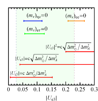
Figure 1: Allowed ranges of $|U_{e3}|$ for the three relations reproduced here in explicit models. The shaded area is the current $3\sigma$ range of $|U_{e3}|$. Also shown are the currently allowed $3\sigma$ ranges corresponding to $|U_{e3}|=c\,\sqrt{\mbox{$\Delta m^{2}_{\odot}$}/\mbox{$\Delta m^{2}_{\rm A}$}}$, $|U_{e3}|^{2}=c\,\sqrt{\mbox{$\Delta m^{2}_{\odot}$}/\mbox{$\Delta m^{2}_{\rm A}$}}$ and $|U_{e3}|=c\,\mbox{$\Delta m^{2}_{\odot}$}/\mbox{$\Delta m^{2}_{\rm A}$}$, where $c$ is varied between 0.25 and 4. Note that the relation $|U_{e3}|=c\,\mbox{$\Delta m^{2}_{\odot}$}/\mbox{$\Delta m^{2}_{\rm A}$}$ is not considered in this paper, but given here for completeness as it also reproduces the data very well.

We propose here very simple and straightforward realizations of the observations made above, namely

$$|U_{e3}|^{2}=\sqrt{\frac{\mbox{$\Delta m^{2}_{\odot}$}}{\mbox{$\Delta m^{2}_{\rm A}$}}}\,\sin^{2}\theta_{12}=0.054_{-0.011}^{+0.016}\,,$$ (3)

and

$$\begin{array}[]{c}\displaystyle|U_{e3}|\simeq\frac{1}{2}\,\sqrt{\frac{\mbox{$\Delta m^{2}_{\odot}$}}{\mbox{$\Delta m^{2}_{\rm A}$}}}\,\sin 2\theta_{12}\cot\theta_{23}=0.078_{-0.025}^{+0.040}\,,\\ \displaystyle|U_{e3}|\simeq\frac{1}{2}\,\sqrt{\frac{\mbox{$\Delta m^{2}_{\odot}$}}{\mbox{$\Delta m^{2}_{\rm A}$}}}\,\sin 2\theta_{12}\tan\theta_{23}=0.084_{-0.027}^{+0.041}\,.\end{array}$$ (4)

These relations are obtained by setting in the normal mass ordering the smallest neutrino mass to zero and by asking the $ee$, $e\mu$ or $e\tau$ element of the neutrino mass matrix in the flavor basis to vanish. We stress that other possibilities for similar relations surely exist, but here we focus on these very simple ones. Our main motivation is to note the potential link of ratios of fermion masses and $U_{e3}$ as an alternative approach in model building.

In what follows we will analyze the predictions of these relations and present simple flavor symmetry models, based on the discrete groups $S_{3}$ and $D_{4}$, respectively, which reproduce them. As mentioned above, we will obtain our relations by combining the single texture zero approach [14] in the flavor basis with the case of a vanishing neutrino mass [15]. The relations we will obtain are simple, and have of course been present in the literature before, see for instance Ref. [16]. However, as far as we know they were neither presented with the motivation that we outlined above, nor with any underlying flavor symmetry model input.

The outline of the paper is as follows: in Section 2 we will analyze the relations (3) and (4) in a model-independent way. Simple models predicting them are discussed in Section 3, before we conclude in Section 4. Some necessary flavor group details are delegated to the Appendix.

2 General Analysis

The lepton mixing matrix can be parameterized as

$$\begin{split}U&=\begin{pmatrix}c_{12}c_{13}&s_{12}c_{13}&s_{13}e^{-i\delta}\\ -c_{23}s_{12}-s_{23}s_{13}c_{12}e^{i\delta}&c_{23}c_{12}-s_{23}s_{13}s_{12}e^{i\delta}&s_{23}c_{13}\\ s_{23}s_{12}-c_{23}s_{13}c_{12}e^{i\delta}&-s_{23}c_{12}-c_{23}s_{13}s_{12}e^{i\delta}&c_{23}c_{13}\end{pmatrix}\mathrm{diag}(1,e^{i\alpha_{1}},e^{i\alpha_{2}})\,.\end{split}$$

Note that we will work in this section in the flavor basis, i.e. the charged lepton mass matrix is diagonal. The neutrino mass matrix is given by

$$m_{\nu}=U\,\mathrm{diag}(m_{1},m_{2},m_{3})\,U^{T}\,.$$ (5)

In the normal hierarchy case, setting the smallest neutrino mass $m_{1}$ to zero and asking the $\alpha\beta$ entry of the mass matrix to vanish, corresponds to the relation

$$U_{\alpha 2}\,U_{\beta 2}\,m_{2}+U_{\alpha 3}\,U_{\beta 3}\,m_{3}=0\,.$$ (6)

This in turn gives two relations which describe the phenomenological results of the scenario, one for the absolute value

$$\frac{\left|U_{\alpha 3}\,U_{\beta 3}\right|}{\left|U_{\alpha 2}\,U_{\beta 2}\right|}=\frac{m_{2}}{m_{3}}=\sqrt{\frac{\mbox{$\Delta m^{2}_{\odot}$}}{\mbox{$\Delta m^{2}_{\rm A}$}}}\,,$$ (7)

and one for the phases

$${\rm arg}(U_{\alpha 3}\,U_{\beta 3}\,U_{\alpha 2}^{\ast}\,U_{\beta 2}^{\ast})=\pi\,.$$ (8)

The first relation (7) will give a constraint on the value of $|U_{e3}|$, the second relation (8) can relate the two physical CP phases with each other. Note that with $m_{1}=0$ only one Majorana phase is present. Simple modifications of the above relations can be made in case the inverted hierarchy is considered, but for the sake of brevity we will not give the relevant expressions here.

Consider now the case of setting the $ee$ element of the neutrino mass matrix to zero. With $\alpha=\beta=e$, the result from Eq. (7) is

$$\tan^{2}\theta_{13}=\sqrt{\frac{\mbox{$\Delta m^{2}_{\odot}$}}{\mbox{$\Delta m^{2}_{\rm A}$}}}\,\sin^{2}\theta_{12}\,,$$ (9)

which with $\tan^{2}\theta_{13}\simeq|U_{e3}|^{2}\,(1+|U_{e3}|^{2})$ corresponds to our Eq. (3). The relevant exact expression for the phases from Eq. (8) is

$$\alpha_{1}-\alpha_{2}=\frac{1}{2}\pi-\delta\,.$$ (10)

The allowed range of $|U_{e3}|$ with this scenario is given in Fig. 1. Note that with the $ee$ element of the mass matrix being zero, there will be no contribution to neutrino-less double beta decay from light neutrinos [17].

The next case is when we set the $e\mu$ element of the neutrino mass matrix to zero. This gives at leading order in $|U_{e3}|$ the already quoted result from Eq. (4):

$$|U_{e3}|\simeq\frac{1}{2}\,\sqrt{\frac{\mbox{$\Delta m^{2}_{\odot}$}}{\mbox{$\Delta m^{2}_{\rm A}$}}}\,\sin 2\theta_{12}\cot\theta_{23}\,,$$ (11)

and furthermore, again at leading order,

$$\alpha_{1}-\alpha_{2}\simeq\frac{1}{2}(\pi-\delta)\,.$$ (12)

The third case occurs for a vanishing $e\tau$ element of $m_{\nu}$, for which we get the same result as for a vanishing $e\mu$ element, with the replacement $\cot\theta_{23}\to\tan\theta_{23}$ and

$$\alpha_{1}-\alpha_{2}\simeq-\frac{1}{2}\delta\,.$$ (13)

The predictions for $|U_{e3}|$ are shown in Fig. 1. The dependence on the atmospheric neutrino parameter $\sin^{2}\theta_{23}$ is displayed in Fig. 2. Note that there is no dependence on this parameter when the $ee$ element is zero.

Let us remark that the predictions are very stable under corrections of renormalization group running.

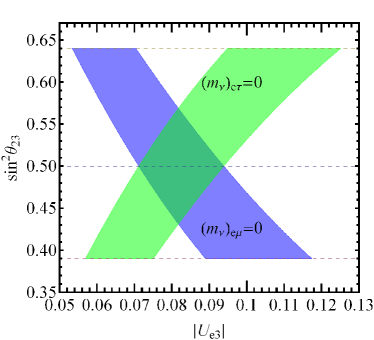
Figure 2: The dependence of $|U_{e3}|$ on $\sin^{2}\theta_{23}$ for the cases of vanishing $m_{1}$ and a zero $e\mu$ ($e\tau$) element of the mass matrix.

In principle our analysis could be extended to cases for which the remaining entries of the mass matrix are zero. It is easy to see that if the smallest mass $m_{1}$ in the normal hierarchy is zero, the $\mu\mu$, $\mu\tau$ and $\tau\tau$ elements cannot vanish. In the inverted hierarchy case with $m_{3}=0$, the $ee$ element cannot be zero. The remaining possibilities in the inverted hierarchy suffer from little predictivity and do not link the ratio of mass-squared differences and $U_{e3}$ in a straightforward manner. For instance, if we would set in the inverted hierarchy case with $m_{3}=0$ the $e\mu$ element of the mass matrix to zero, we would get

$$|U_{e3}|\,\cos\delta\simeq\frac{1}{4}\frac{\mbox{$\Delta m^{2}_{\odot}$}}{\mbox{$\Delta m^{2}_{\rm A}$}}\frac{\sin 2\theta_{12}}{\tan\theta_{23}}\,.$$

A similar relation holds for the $\mu\tau$ block of $m_{\nu}$, setting for instance the $\mu\mu$ entry to zero yields

$$|U_{e3}|\,\cos\delta\simeq\frac{1}{4}\frac{\mbox{$\Delta m^{2}_{\odot}$}}{\mbox{$\Delta m^{2}_{\rm A}$}}\frac{\cos 2\theta_{12}\,\tan\theta_{12}}{\cos^{2}\theta_{12}\,\tan\theta_{23}}\,.$$

This can be traced back to the fact that when $m_{3}=0$ the only remaining masses are $m_{2}\simeq m_{1}$, i.e. they do not possess a hierarchy and do not allow to make a straightforward and direct relation between $|U_{e3}|$ and a small ratio, simply because there is no small ratio of masses.

3 Simple Model Realizations

In this section we present several examples of flavor models which produce the desired features of the relations in Eqs. (3, 4). The key ingredients to get these relations are the vanishing elements in the Majorana mass matrix $m_{\nu}$ and one massless state in the active neutrino spectrum. The latter property is naturally explained by a seesaw mechanism with two right-handed neutrinos [18], see [19] for a review. We attribute the former property to texture zeros in the Dirac and the Majorana mass matrices in the original Lagrangian at some high-energy scale. The texture zeros are realized along the line of [20, 21], where the discrete flavor symmetries and their breakdown by new scalar fields play the central role.

3.1 A Model for $(m_{\nu})_{ee}=0$

Let us first discuss a model which produces Eq. (3). We introduce $S_{3}\times Z_{3}$ as a discrete flavor symmetry and require the presence of scalar fields which carry nontrivial charges of the flavor symmetry. The particle content relevant for lepton masses and mixings are summarized in the following table:

	$(\overline{L_{1}},\overline{L_{2}})$	$\overline{L_{3}}$	$(\nu_{R_{1}},\nu_{R_{2}})$	$e_{R}$	$\mu_{R}$	$\tau_{R}$	$(\phi_{1},\phi_{2})$	$\chi$
$S_{3}$	$2^{*}$	$1_{\rm S}$	$2$	$1_{\rm S}$	$1_{\rm S}$	$1_{\rm S}$	$2$	$1_{\rm S}$
$Z_{3}$	$\omega$	$\omega$	$\omega$	$\omega$	$1$	$\omega^{2}$	$\omega$	$\omega$

Here $\omega=e^{2\pi i/3}$, $L_{i}$ are the left-handed lepton doublets, $\nu_{R_{i}}$ are the right-handed neutrinos, $e_{R},\mu_{R},\tau_{R}$ are the right-handed charged leptons. The scalar fields $\phi_{1,2}$ and $\chi$ are so-called flavons, which are singlet under the Standard Model gauge group and whose vacuum expectation value (VEV) break the flavor symmetry. Details for the tensor products of $S_{3}$ are presented in Appendix A.1.

At the energy scales where the flavor symmetries are unbroken, the neutrino Yukawa interactions and the Majorana masses for $\nu_{R_{i}}$ are written in terms of higher-dimensional operators which involve the Standard Model fields and the flavons. At the leading order of the inverse power of the cutoff scale, they are given by

$$-\mathcal{L}_{\nu} \,=\, y_{1}\,(\overline{L_{1}}\nu_{R_{1}}+\overline{L_{2}}\nu_{R_{2}})\chi H^{*}\,+\,y_{2}\,(\overline{L_{1}}\nu_{R_{2}}\phi_{2}+\overline{L_{2}}\nu_{R_{1}}\phi_{1})H^{*}$$

$$\,+\,y_{3}\,\overline{L_{3}}(\nu_{R_{1}}\phi_{2}+\nu_{R_{2}}\phi_{1})H^{*}\,+\,\frac{1}{2}g_{1}(\overline{\nu_{R_{1}}^{c}}\nu_{R_{1}}\phi_{1}+\overline{\nu_{R_{2}}^{c}}\nu_{R_{2}}\phi_{2})$$

$$\,+\,\frac{1}{2}g_{2}(\overline{\nu_{R_{1}}^{c}}\nu_{R_{2}}+\overline{\nu_{R_{2}}^{c}}\nu_{R_{1}})\chi\,+\,{\rm h.c.},$$

where $H$ is the standard model Higgs field, $y_{i}$ are coupling constants which carry inverse mass dimension, while $g_{i}$ are dimensionless constants. After $\phi_{i}$ and $\chi$ obtain vacuum expectation values according to the alignment

$$\phi_{i}\to\begin{pmatrix}\langle\phi_{1}\rangle\\ 0\\ \end{pmatrix},\quad\chi\to\langle\chi\rangle,$$ (15)

and electroweak symmetry breaking $H\to\langle H\rangle=(v,0)^{\rm T}$, the mass matrices at low energy take the forms

$$m_{D}\simeq\begin{pmatrix}a&0\\ b&a\\ 0&c\\ \end{pmatrix},\quad M_{R}\simeq\begin{pmatrix}M_{A}&M_{B}\\ M_{B}&0\\ \end{pmatrix},$$ (16)

where $a=y_{1}\langle\chi\rangle v$, $b=y_{2}\langle\phi_{1}\rangle v$, $c=y_{3}\langle\phi_{1}\rangle v$, $M_{A}=g_{1}\langle\phi_{1}\rangle$ and $M_{B}=g_{2}\langle\chi\rangle$. By assuming $m_{D}\ll M_{R}$ and performing the seesaw diagonalization, one finds the effective Majorana mass matrix

$$m_{\nu}\,\simeq\,\begin{pmatrix}0&a^{2}&ac\\ a^{2}&2ab&bc\\ ac&bc&0\\ \end{pmatrix}\frac{1}{M_{B}}\,-\,\begin{pmatrix}0&0&0\\ 0&a^{2}&ac\\ 0&ac&c^{2}\\ \end{pmatrix}\frac{M_{A}}{M_{B}^{2}}\,.$$ (17)

The charged leptons are diagonal in this model (see below). The vanishing of $(m_{\nu})_{ee}$ is thus realized due to the texture zeros in the Dirac and the Majorana mass matrices. Notice that the texture (16) is equivalent to one of the patterns discussed in [22] and its physical implications are already studied. Central values of the mass-squared differences and the solar and atmospheric mixing angles are obtained for instance by setting $a/\sqrt{M_{B}}\simeq 0.079\,{\rm eV^{1/2}}$, $b/\sqrt{M_{B}}\simeq 0.013\,{\rm eV^{1/2}}$ with the conditions $c\simeq b$, $M_{A}\simeq-M_{B}$. Since our purpose here is to present an example for a model leading to $(m_{\nu})_{ee}=0$, we do not discuss (17) further.

The charged lepton sector is written by a combination of higher-dimensional operators and a renormalizable operator. At leading order of the inverse of the cutoff, it is given by

$$-\mathcal{L}_{l} \,=\, y_{e}\,(\overline{L_{1}}\phi_{1}+\overline{L_{2}}\phi_{2})e_{R}H,+\,y_{\mu}\,(\overline{L_{1}}\phi_{2}^{*}+\overline{L_{2}}\phi_{1}^{*})\mu_{R}H\,+\,y_{\tau}\,\overline{L_{3}}\,\tau_{R}H\,+\,{\rm h.c.},$$

where $y_{e}$ and $y_{\mu}$ are parameters of inverse mass dimension while $y_{\tau}$ is dimensionless. In the vacuum Eq. (15), the charged lepton mass matrix is diagonal

$$M_{l}\simeq\begin{pmatrix}y_{e}\langle\phi_{1}\rangle&0&0\\ 0&y_{\mu}\langle\phi_{1}\rangle^{*}&0\\ 0&0&y_{\tau}\end{pmatrix}v.$$ (18)

Due to the effective nature of the muon mass term, the hierarchy between $m_{\mu}$ and $m_{\tau}$ is naturally explained. The smaller electron mass can easily be explained by adding an additional $U(1)$ symmetry under which the right-handed electron field is charged.

For the realization of desired flavor structure, the “asymmetric” VEV configuration $\phi_{i}\to(\langle\phi_{1}\rangle,0)^{\rm T}$ in Eq. (15) is playing a vital role. Such an alignment has been shown to be easily possible in generic potentials in $S_{3}$ theories in Ref. [20]. Furthermore, in Refs. [23] it was shown to achieve the required alignment via boundary conditions of scalar fields in extra-dimensional space, which force either of the two components to have a zero mode.

3.2 Models for $(m_{\nu})_{e\mu}=0$ and $(m_{\nu})_{e\tau}=0$

Next we present a model for Eq. (4). We assume $S_{3}\times Z_{4}$ flavor symmetry and introduce gauge singlet scalars $\xi_{1},\xi_{2}$ and $\eta$. The charge assignment is as follows:

	$(\overline{L_{1}},\overline{L_{2}})$	$\overline{L_{3}}$	$\nu_{R_{1}}$	$\nu_{R_{2}}$	$e_{R}$	$\mu_{R}$	$\tau_{R}$	$(\xi_{1},\xi_{2})$	$\eta$
$S_{3}$	$2$	$1_{\rm S}$	$1_{\rm S}$	$1_{\rm S}$	$1_{\rm A}$	$1_{\rm A}$	$1_{\rm S}$	$2$	$1_{\rm S}$
$Z_{4}$	$i$	$i$	$1$	$-1$	$1$	$-1$	$-i$	$i$	$i$

At leading order of the inverse of the cutoff scale, the flavor-symmetric neutrino Yukawa Lagrangian is written as

$$-\mathcal{L}_{\nu} \,=\, z_{1}\,(\overline{L_{1}}\xi_{1}^{*}+\overline{L_{2}}\xi_{2}^{*})\nu_{R_{1}}H^{*}\,+\,z_{2}\,(\overline{L_{1}}\xi_{2}+\overline{L_{2}}\xi_{1})\nu_{R_{2}}H^{*}$$

$$\,+\,z_{3}\,\overline{L_{3}}\,\nu_{R_{1}}\eta^{*}H^{*}\,+\,z_{4}\,\overline{L_{3}}\,\nu_{R_{2}}\eta H^{*}$$

$$\,+\,\frac{1}{2}(M_{1}\overline{\nu_{R_{1}}^{c}}\nu_{R_{1}}+M_{2}\overline{\nu_{R_{2}}^{c}}\nu_{R_{2}})\,+\,{\rm h.c.},$$

where $z_{i}$ are coupling constants which carry inverse mass dimension and $M_{1,2}$ are the Majorana masses for the right-handed neutrinos. After the doublet $(\xi_{1},\xi_{2})$ and the singlet $\eta$ develop the vacuum expectation values

$$\xi_{i}\to\begin{pmatrix}\langle\xi_{1}\rangle\\ 0\\ \end{pmatrix},\quad\eta\to\langle\eta\rangle,$$ (20)

and the electroweak symmetry breaks down, the neutrino mass matrices are given by

$$m_{D}\simeq\begin{pmatrix}p&0\\ 0&q\\ r&s\\ \end{pmatrix},\quad M_{R}\simeq\begin{pmatrix}M_{1}&0\\ 0&M_{2}\\ \end{pmatrix},$$ (21)

where $p=z_{1}\langle\xi_{1}\rangle^{*}v$, $q=z_{2}\langle\xi_{1}\rangle v$, $r=z_{3}\langle\eta\rangle^{*}v$, and $s=z_{4}\langle\eta\rangle v$. If $p,q,r,s\ll M_{1,2}$ so that the seesaw mechanism works, the mass matrix for the left-handed neutrinos reads

$$m_{\nu}\,\simeq\,\begin{pmatrix}p^{2}&0&pr\\ 0&0&0\\ pr&0&r^{2}\\ \end{pmatrix}\frac{1}{M_{1}}\,+\,\begin{pmatrix}0&0&0\\ 0&q^{2}&qs\\ 0&qs&s^{2}\\ \end{pmatrix}\frac{1}{M_{2}}\,.$$ (22)

The charged lepton mass matrix is again diagonal, and is just as in the previous subsection given by a combination of renormalizable terms for the tau lepton mass and effective terms for the electron and muon mass. The vanishing of $(m_{\nu})_{e\mu}$ is achieved by the texture zeros in the Dirac and the Majorana mass matrices (21). We note that such textures have been discussed in [24].

With the simple replacement $L_{2}\leftrightarrow L_{3}$ one can modify the model to generate $(m_{\nu})_{e\tau}=0$.

Another model to obtain a vanishing $(m_{\nu})_{e\mu}$ uses the flavor group $D_{4}\times Z_{2}$:

	$(\overline{L_{1}},\overline{L_{2}})$	$\overline{L_{3}}$	$(\nu_{R_{1}},\nu_{R_{2}})$	$(e_{R},\mu_{R})$	$\tau_{R}$	$\eta_{1}^{-}$	$\eta_{2}^{+}$	$\eta_{3}^{+}$	$\eta_{4}^{-}$	$(\xi_{1}^{+},\xi_{2}^{+})$
$D_{4}$	$2$	$1_{1}$	$2$	$2$	$1_{1}$	$1_{1}$	$1_{2}$	$1_{3}$	$1_{4}$	$2$
$Z_{2}$	$+$	$+$	$+$	$-$	$+$	$-$	$+$	$+$	$-$	$+$

With this identification and the multiplication rules in the convention of Ref. [25] (see Appendix A.2), it is straightforward to see that the charged lepton and the right-handed neutrino mass matrices are diagonal, while the Dirac mass matrix has a texture as in (21). In contrast to the $S_{3}$ model, there is no VEV alignment necessary, at the price however of introducing 6 weak doublets $\eta_{1}^{-}$, $\eta_{2}^{+}$, $\eta_{3}^{+}$, $\eta_{4}^{-}$ and $(\xi_{1}^{+},\xi_{2}^{+})$.

4 Summary and Conclusions

We stressed here that the recently emerging non-zero $\theta_{13}$ puts some pressure on models with an initially vanishing value, and that it may be natural that the two small but non-zero quantities in neutrino oscillations, $U_{e3}$ and the ratio of mass-squared differences, are linked. Indeed, the ratio of mass-squared differences is numerically close to the value of $U_{e3}$. The most straightforward application of this idea leads to the relations $|U_{e3}|^{2}=\sqrt{\mbox{$\Delta m^{2}_{\odot}$}/\mbox{$\Delta m^{2}_{\rm A}$}}\,\sin^{2}\theta_{12}\simeq 0.05$ and $|U_{e3}|\simeq\frac{1}{2}\,\sqrt{\mbox{$\Delta m^{2}_{\odot}$}/\mbox{$\Delta m^{2}_{\rm A}$}}\,\sin 2\theta_{12}\simeq 0.08$, in good agreement with data. There may be other realizations of this and similar observations, and interesting model building opportunities, somewhat alternative to the usual considerations, may arise.

Acknowledgments

WR is supported by the ERC under the Starting Grant MANITOP and by the DFG in the Transregio 27, MT is supported by the Grand-in-Aid for Scientific Research No. 21340055, and AW by the Young Researcher Overseas Visits Program for Vitalizing Brain Circulation Japanese in JSPS No. R2209.

Appendix A Group Details

For the sake of completeness, we give here the necessary details to reproduce the models in Section 3. The complete group structure can be found in Ref. [20] for $S_{3}$ and [25] for $D_{4}$.

A.1 The group $S_{3}$

We use here the complex representation of $S_{3}$, see for instance Ref. [20]. With $S_{3}$ doublets $\psi=\begin{pmatrix}\psi_{1}\\ \psi_{2}\\ \end{pmatrix}$ and $\phi=\begin{pmatrix}\phi_{1}\\ \phi_{2}\\ \end{pmatrix}$, $2\times 2$ is decomposed as

$$\psi^{*}\times\phi=\underbrace{\begin{pmatrix}\psi_{1}^{*}\phi_{2}\\ \psi_{2}^{*}\phi_{1}\\ \end{pmatrix}}_{2}+\underbrace{(\psi_{1}^{*}\phi_{1}-\psi_{2}^{*}\phi_{2})}_{1_{\rm A}}+\underbrace{(\psi_{1}^{*}\phi_{1}+\psi_{2}^{*}\phi_{2})}_{1_{\rm S}}\,,$$

and

$$\psi\times\phi=\underbrace{\begin{pmatrix}\psi_{2}\phi_{2}\\ \psi_{1}\phi_{1}\\ \end{pmatrix}}_{2}+\underbrace{(\psi_{1}\phi_{2}-\psi_{2}\phi_{1})}_{1_{\rm A}}+\underbrace{(\psi_{1}\phi_{2}+\psi_{2}\phi_{1})}_{1_{\rm S}}\,.$$

A.2 The group $D_{4}$

In the convention used here, the four singlets of $D_{4}$ multiply as follows:

$\times$	$1_{1}$	$1_{2}$	$1_{3}$	$1_{4}$
$1_{1}$	$1_{1}$	$1_{2}$	$1_{3}$	$1_{4}$
$1_{2}$	$1_{2}$	$1_{1}$	$1_{4}$	$1_{3}$
$1_{3}$	$1_{3}$	$1_{4}$	$1_{1}$	$1_{2}$
$1_{4}$	$1_{4}$	$1_{3}$	$1_{2}$	$1_{1}$

Two doublets $(\psi_{1},\psi_{2})^{\rm T}$ and $(\phi_{1},\phi_{2})^{\rm T}$ multiply as $2\times 2=1_{1}+1_{2}+1_{3}+1_{4}$, where

$$(\psi_{1}\phi_{1}+\psi_{2}\phi_{2})/\sqrt{2}\sim 1_{1}\;,\;\;\;(\psi_{1}\phi_{2}+\psi_{2}\phi_{1})/\sqrt{2}\sim 1_{2}\,,$$

$$(\psi_{1}\phi_{2}-\psi_{2}\phi_{1})/\sqrt{2}\sim 1_{3}\;,\;\;\;(\psi_{1}\phi_{1}-\psi_{2}\phi_{2})/\sqrt{2}\sim 1_{4}\,.$$

References

- [1] M. Apollonio et al. [CHOOZ Collaboration], Phys. Lett. B 466 (1999) 415 [hep-ex/9907037].
- [2] G. L. Fogli, E. Lisi, A. Marrone, A. Palazzo and A. M. Rotunno, Phys. Rev. Lett. 101 (2008) 141801 [arXiv:0806.2649 [hep-ph]].
- [3] M. C. Gonzalez-Garcia, M. Maltoni and J. Salvado, JHEP 1004 (2010) 056 [arXiv:1001.4524 [hep-ph]].
- [4] T. Schwetz, M. Tortola and J. W. F. Valle, New J. Phys. 13 (2011) 063004 [arXiv:1103.0734 [hep-ph]].
- [5] G. L. Fogli, E. Lisi, A. Marrone, A. Palazzo and A. M. Rotunno, Phys. Rev. D 84 (2011) 053007 [arXiv:1106.6028 [hep-ph]].
- [6] T. Schwetz, M. Tortola and J. W. F. Valle, New J. Phys. 13 (2011) 109401 [arXiv:1108.1376 [hep-ph]].
- [7] P. A. N. Machado, H. Minakata, H. Nunokawa and R. Z. Funchal, arXiv:1111.3330 [hep-ph].
- [8] K. Abe et al. [T2K Collaboration], Phys. Rev. Lett. 107 (2011) 041801 [arXiv:1106.2822 [hep-ex]].
- [9] P. Adamson et al. [MINOS Collaboration], Phys. Rev. Lett. 107 (2011) 181802 [arXiv:1108.0015 [hep-ex]].
- [10] Y. Abe et al. [DOUBLE-CHOOZ Collaboration], arXiv:1112.6353 [hep-ex].
- [11] G. Altarelli and F. Feruglio, Rev. Mod. Phys. 82 (2010) 2701 [arXiv:1002.0211 [hep-ph]].
- [12] H. Ishimori, T. Kobayashi, H. Ohki, Y. Shimizu, H. Okada and M. Tanimoto, Prog. Theor. Phys. Suppl. 183 (2010) 1 [arXiv:1003.3552 [hep-th]].
- [13] R. Gatto, G. Sartori and M. Tonin, Phys. Lett. B 28 (1968) 128.
- [14] A. Merle and W. Rodejohann, Phys. Rev. D 73 (2006) 073012 [arXiv:hep-ph/0603111 [hep-ph]].
- [15] G. C. Branco, R. Gonzalez Felipe, F. R. Joaquim and T. Yanagida, Phys. Lett. B 562 (2003) 265 [hep-ph/0212341].
- [16] E. I. Lashin and N. Chamoun, arXiv:1108.4010 [hep-ph].
- [17] W. Rodejohann, Int. J. Mod. Phys. E 20 (2011) 1833 [arXiv:1106.1334 [hep-ph]].
- [18] P. H. Frampton, S. L. Glashow and T. Yanagida, Phys. Lett. B 548 (2002) 119 [hep-ph/0208157].
- [19] W. -l. Guo, Z. -z. Xing and S. Zhou, Int. J. Mod. Phys. E 16 (2007) 1 [hep-ph/0612033].
- [20] N. Haba and K. Yoshioka, Nucl. Phys. B 739 (2006) 254 [hep-ph/0511108].
- [21] S. Kaneko, H. Sawanaka, T. Shingai, M. Tanimoto and K. Yoshioka, Prog. Theor. Phys. 117 (2007) 161 [hep-ph/0609220]; hep-ph/0611057; hep-ph/0703250; Int. J. Mod. Phys. E 16 (2007) 1427.
- [22] S. Goswami and A. Watanabe, Phys. Rev. D 79 (2009) 033004 [arXiv:0807.3438 [hep-ph]]; S. Goswami, S. Khan and A. Watanabe, Phys. Lett. B 693 (2010) 249 [arXiv:0811.4744 [hep-ph]].
- [23] N. Haba, A. Watanabe and K. Yoshioka, Phys. Rev. Lett. 97 (2006) 041601 [hep-ph/0603116]; T. Kobayashi, Y. Omura and K. Yoshioka, Phys. Rev. D 78 (2008) 115006 [arXiv:0809.3064 [hep-ph]].
- [24] S. Goswami, S. Khan and W. Rodejohann, Phys. Lett. B 680 (2009) 255 [arXiv:0905.2739 [hep-ph]].
- [25] C. Hagedorn and W. Rodejohann, JHEP 0507 (2005) 034 [hep-ph/0503143].