Neutrino production coherence and oscillation experiments

Abstract

Neutrino oscillations are only observable when the neutrino production, propagation and detection coherence conditions are satisfied. In this paper we consider in detail neutrino production coherence, taking $\pi\to\mu\nu$ decay as an example. We compare the oscillation probabilities obtained in two different ways: (1) coherent summation of the amplitudes of neutrino production at different points along the trajectory of the parent pion; (2) averaging of the standard oscillation probability over the neutrino production coordinate in the source. We demonstrate that the results of these two different approaches exactly coincide, provided that the parent pion is considered as pointlike and the detection process is perfectly localized. In this case the standard averaging of the oscillation probability over the finite spatial extensions of the neutrino source (and detector) properly takes possible decoherence effects into account. We analyze the reason for this equivalence of the two approaches and demonstrate that for pion wave packets of finite width $\sigma_{x\pi}$ the equivalence is broken. The leading order correction to the oscillation probability due to $\sigma_{x\pi}\neq 0$ is shown to be $\sim[v_{g}/(v_{g}-v_{\pi})]\sigma_{x\pi}/l_{\rm osc}$, where $v_{g}$ and $v_{\pi}$ are the group velocities of the neutrino and pion wave packets, and $l_{\rm osc}$ is the neutrino oscillation length.

1 Introduction

It is well known that neutrino oscillations are only observable when the conditions of coherent production, propagation and detection of different neutrino mass eigenstates are satisfied. The production and detection coherence conditions ensure that the intrinsic quantum-mechanical energy uncertainties at neutrino production and detection are large compared to the energy difference $\Delta E_{jk}$ of different neutrino mass eigenstates:

$$\Delta E_{jk}\sim\frac{\Delta m_{jk}^{2}}{2E}\ll\sigma_{E}\,,$$ (1)

where $\sigma_{E}=\min\{\sigma_{E}^{\rm prod},\,\sigma_{E}^{\rm det}\}$. If this condition is violated, the neutrino production or detection process will be able to discriminate between different neutrino mass eigenstates, thus destroying neutrino oscillations. Indeed, neutrino mass eigenstates do not oscillate in vacuum, and the oscillations are only possible because neutrinos are emitted and detected as flavour states – coherent linear superpositions of different mass eigenstates. This coherence is destroyed if the condition (1) is violated. Production/detection coherence is known to be related to the localization of the corresponding neutrino emission and absorption processes, as it is the localization of these processes that determines the energy uncertainty $\sigma_{E}$ [1].

The propagation decoherence can take place if neutrinos propagate very long distances. It is related to the fact that the wave packets describing the different neutrino mass eigenstates that compose a flavour state propagate with different group velocities, and therefore after a long enough time they cease to overlap and separate to such an extent that the amplitudes of their interaction with the detector particles cannot interfere. For ultrarelativistic neutrinos the propagation coherence condition can be written as

$$\frac{\Delta m_{jk}^{2}}{2E^{2}}L\ll\sigma_{x\nu}\simeq v_{g}/\sigma_{E}\,,$$ (2)

where $L$ is the baseline, $v_{g}$ is the average group velocity of the wave packets of different neutrino mass eigenstates and $\sigma_{x\nu}$ is their common effective spatial width. Note that both the production/detection and propagation coherence conditions, eqs. (1) and (2), put upper limits on the mass squared differences $\Delta m_{jk}^{2}$ of different neutrino mass eigenstates.

In practice, the propagation coherence condition is very well satisfied in all cases except for neutrinos of astrophysical or cosmological origin, such as solar, supernova or relic neutrinos. As to the production/detection coherence condition, it is usually tacitly assumed to be always satisfied due to the extreme smallness of the neutrino masses (and therefore of their mass squared differences). However, there may exist situations in which this is not the case. In particular, in view of possible existence of sterile neutrinos with masses in the eV, keV or even MeV range, the question of production/detection coherence should be analyzed especially carefully when the corresponding mass squared differences are involved. Note that there are some hints for such sterile neutrinos coming from short-baseline accelerator experiments, the reactor neutrino anomaly, gallium radiative source experiments, $r$-process supernova nucleosynthesis, pulsar kicks, warm dark matter and leptogenesis scenarios [2].

The issue of coherence is of utmost importance for neutrino oscillation experiments. If the coherence conditions are strongly violated, the probabilities of flavour transitions will correspond to averaged out oscillations, i.e. they will have neither $L$ nor $E$ dependence. This means that the two most important signatures of neutrino oscillations – the dependence on the distance between the neutrino source and detector and the distortion of the energy spectrum of the detected signal – will be absent. In particular, the two-detector setups of neutrino oscillation experiments will be completely useless. In such situations one would have to rely entirely on the overall normalization of the neutrino flux, which is usually known with insufficient accuracy.

The question of neutrino production coherence has been recently addressed in ref. [3], where it was considered in the framework of incoherent summation of probabilities of neutrino production at different points inside the neutrino source. In addition, a simplified study of the coherent amplitude summation was performed in that paper. It was demonstrated that under certain conditions the two summation procedures lead to identical results.

In this paper we address this question within a more rigorous and consistent approach. We study in detail neutrino production coherence, taking $\pi\to\mu\nu$ decay as an example. With minimal modifications, our analysis will also be applicable to neutrino detection. We find the oscillations probabilities in two different approaches:

• An approach based on the quantum-mechanical wave packet formalism. We first calculate the transition amplitude by summing the amplitudes corresponding to neutrino production in pion decay at different points along the trajectory of the parent pion. We then calculate the transition probability and study its coherence properties.

• We assume that for each individual neutrino production event the oscillation probability is fully coherent but depends on the exact position of the neutrino production point, i.e. is described by the standard oscillation formula. The effective oscillation probability is then found by integrating (averaging) this standard coordinate-dependent probability along the neutrino source, with the proper exponential factor describing the pion decay included [3].

It should be stressed that, strictly speaking, the first approach, based on a quantum mechanical amplitude summation, should always be used. The second (probability) summation procedure, which is classical in nature, is however much simpler and is usually employed in the analyses of experiments. It is therefore one of the main goals of the present paper to study if and when the use of the probability summation approach is indeed justified.

We compare the results of the two approaches and demonstrate that they exactly coincide when the parent pions are considered as pointlike particles and the detection process is perfectly localized in space and time. One can therefore conclude that for pointlike parent particles and well-localized detection the standard averaging of the oscillation probabilities over the finite spatial extensions of the neutrino source (and detector) properly takes possible decoherence effects into account. We analyze the reason for this equivalence of the two approaches and demonstrate that for finite-size pion wave packets the equivalence is broken. We show that for small widths of the pion wave packets $\sigma_{x\pi}$ the oscillation probabilities get small oscillatory corrections which are linear in $\sigma_{x\pi}$. For different shapes of the pion wave packets these corrections have the same form and differ only by numerical coefficients. At the same time, large $\sigma_{x\pi}$ can lead to production decoherence and thus to suppression of the oscillations. We also consider the production coherence in the case when the charged leptons accompanying neutrino production are detected, leading to neutrino tagging, as well as in the case when the interactions of pions in the bunch between themselves or with other particles which may be present in the neutrino source are taken into account.

A note on terminology. In this paper we use the word ‘coherence’ in two different, though related, senses. By production coherence we mean that different neutrino mass eigenstates are produced coherently, so that the emitted neutrino is a flavour eigenstate. By coherent summation we mean the summation of the amplitudes of neutrino production at different points along the trajectory of the parent pion. As we shall see, these two coherences are in fact acting in opposite directions: if the production is incoherent, then the coherent summation (i.e. approach 1 discussed above) is mandatory, whereas for coherent neutrino production the incoherent probability summation (approach 2) is justified. The common feature of the two coherences is that both require summation of certain amplitudes. Indeed, in the case of neutrino production coherence, these are the amplitudes of emission of different neutrino mass eigenstates, whereas in the case of coherent summation approach, these are the amplitudes of neutrino emission from different space-time points.

The paper is organized as follows. In section 2 we calculate the oscillation probability for neutrinos produced in decays of pointlike pions in a decay tunnel. The calculations are performed in the quantum-mechanical wave packet approach with summation of the amplitudes of neutrino production at different points along the tunnel. In section 3 we recapitulate how the same problem is solved at the level of summation of probabilities rather than amplitudes. In section 4 we generalize the results of the amplitude summation approach to the case of non-zero spatial width of the pion wave packets. We then consider the particular cases of Gaussian and box-type pion wave packets. In section 5 we apply the probability summation approach to the case of protons incident on a finite-thickness target. We also compare the obtained results with those of section 4. In section 6 we develop an alternative approach to the quantum mechanical amplitude summation calculation, which is valid for arbitrary shapes of the pion wave packets. In section 7 we consider effects of possible detection of the charged lepton accompanying the neutrino production on neutrino production coherence. We also briefly discuss here the effects of the interaction of pions in the bunch between themselves or with other particles which may be present in the neutrino source. Section 8 is devoted to implications of our analysis for various neutrino experiments. We summarize and discuss our results in section 9.

2 Oscillation probabilities in the wave packet approach. Pointlike parent particle approximation

In the quantum-mechanical wave packet approach, the oscillation amplitude ${\cal A}_{\alpha\beta}(L,t)$ is obtained by projecting the evolved neutrino state, which was initially produced as the flavour eigenstate $\nu_{\alpha}$, onto the detected neutrino flavour eigenstate $\nu_{\beta}$. The oscillation probability $P_{\alpha\beta}(L)$ is then found by integrating the squared modulus of ${\cal A}_{\alpha\beta}(L,t)$ over time (see, e.g., [4]).

Let us first consider oscillations of neutrinos produced in decays of quasi-free parent particles. By this we mean that the decaying particles may be confined to a finite-size source or a decay tunnel, but their interactions with each other or with other particles which may be present within the source can be neglected (we will relax these assumptions in section 7). As an example, we take the $\pi\to\mu\nu$ decay. We will treat this problem in a 1-dimensional approach, i.e. assuming that the neutrino momentum ${\mathbf{p}}$ is parallel to the baseline vector ${\mathbf{L}}$ connecting the pion production and neutrino detection points. Such an approximation is well justified when the transverse (i.e. orthogonal to ${\mathbf{L}}$) sizes of the neutrino source and detector are small compared to $L$.

To find the wave function of the produced neutrino state, we will need the wave functions of the parent pion and the muon which participate in the production process.

2.1 The pion and muon wave functions

We will be assuming that pions are produced by a beam of protons incident on a solid-state target and then decay inside a decay tunnel, with the total length of the decay tunnel being $l_{p}$. Such a setup corresponds to accelerator experiments. The nuclei in the target are well localized, with the uncertainty of their position $\sigma_{xN}$ being of the order of inter-atomic distances, $\sigma_{xN}\sim 10^{-8}$ cm. The spatial width of the wave packets of the incident protons $\sigma_{xp}$ depends on the conditions of their production; it cannot exceed the mean distance between the protons in the bunch, and e.g. for the Fermilab NuMI source it can be estimated as $\sigma_{xp}\lesssim 10^{-4}$ cm. The spatial size of the pion production region $\sigma_{xP}$ can be defined as [6, 7]

$$\frac{1}{\sigma_{xP}^{2}}\equiv\frac{1}{\sigma_{xN}^{2}}+\frac{1}{\sigma_{xp}^{2}}\,.$$ (3)

We can also define the effective velocity of the pion production region as the sum of the group velocities $v_{p}$ and $v_{N}$ of the incident proton and the target nucleus, weighted with the inverse squared widths of the corresponding wave packets:

$$v_{P}\equiv\sigma_{xP}^{2}\left(\frac{v_{p}}{\sigma_{xp}^{2}}+\frac{v_{N}}{\sigma_{xN}^{2}}\right).$$ (4)

The coordinate-space width of the pion wave packets can then be found from the relation [6, 7, 8]

$$\sigma_{x\pi}\approx[\sigma_{xP}^{2}+(v_{P}-v_{\pi})^{2}/\sigma_{e\pi}^{2}]^{1/2}\,,$$ (5)

where $v_{\pi}$ and $\sigma_{e\pi}$ are, respectively, the group velocity of the pion wave packet and the energy uncertainty of the produced pion state. The latter is approximately equal to the inverse of the overlap time of the proton and nucleon wave packets at pion production [7]:

$$\sigma_{e\pi}\approx\frac{v_{p}-v_{N}}{(\sigma_{xp}^{2}+\sigma_{xN}^{2})^{1/2}}\approx\frac{v_{p}}{\sigma_{xp}}\,.$$ (6)

Eq. (5) thus has a simple physical meaning: the first term in the square brackets is the contribution of the finite spatial size of the pion production region to the width of the pion wave packet, whereas the second term is related to the fact that the pion production takes finite time.

As follows from (3), the coordinate uncertainty of the pion production point $\sigma_{xP}$ is dominated by the size of the shortest wave packet of the participating particles, which in our case is $\sigma_{xN}$: $\sigma_{xP}\simeq\sigma_{xN}$. We shall also assume that the target nuclei are at rest, $v_{N}=0$. Eq. (4) then gives $v_{P}\approx v_{p}(\sigma_{xN}/\sigma_{xp})^{2}\ll v_{p}$. From eqs. (5) and (6) we find

$$\sigma_{x\pi}\approx\left[\sigma_{xN}^{2}+(v_{\pi}/v_{p})^{2}\,\sigma_{xp}^{2}\right]^{1/2}\,.$$ (7)

Thus, $\sigma_{x\pi}\lesssim\sigma_{xp}\lesssim 10^{-4}$ cm, i.e. the spatial width of the pion wave packet is much smaller than all the lengths of interest in the problem – the length of the decay tunnel $l_{p}$, the baseline $L$ and the oscillation length $l_{\rm osc}=4\pi p/\Delta m^{2}$, where $p$ is the neutrino momentum. Therefore to a very good approximation one can consider the pions as pointlike particles.

Let us recall that the coordinate-space wave packet describing a moving free particle can be written, in the approximation where the spreading of the wave packet is neglected, as

$$\psi(x,t)\simeq e^{ip_{0}x-iE(p_{0})t}g(x-v_{g}t)\,,$$ (8)

where $p_{0}$ is the peak momentum of the wave packet, $v_{g}=(\partial E(p)/\partial p)|_{p_{0}}$ is its group velocity and $g(x-v_{g}t)$ is its shape factor (envelope function) (see, e.g., [9]). The shape factor is the Fourier transform of the momentum distribution amplitude (i.e. of the momentum-space wave function) of the pion; it quickly decreases when $|x-v_{g}t|$ becomes large compared to the spatial width of the wave packet $\sigma_{x}$. Since $g$ depends on $x$ and $t$ only through the combination $x-v_{g}t$, for stable particles eq. (8) describes a wave packet propagating with the group velocity $v_{g}$ without changing its shape. For unstable particles the energy $E(p_{0})$ in eq. (8) should be replaced according to $E(p_{0})\to E(p_{0})-i\Gamma/2$, where $\Gamma$ is the particle’s decay width in the laboratory frame.

As was pointed out above, in the problem under consideration pions can to a very good approximation be regarded as pointlike particles, i.e. the shape factor $g_{\pi}(x-v_{\pi}t)$ of their wave packets can be taken to be a $\delta$-function. The pion wave function then takes the form

$$\psi_{\pi}(x,t)=C_{\pi}\,e^{iQx-iE_{\pi}(Q)t-\Gamma t/2}\,\delta(x-v_{\pi}t)\,{\rm box}(x;l_{p},0)\,,$$ (9)

where $C_{\pi}$ is a normalization constant, $Q$ is the mean momentum of the pion state, $E_{\pi}(Q)=(Q^{2}+m_{\pi}^{2})^{1/2}$, $v_{\pi}$ is the group velocity of the pion wave packet, and the function ${\rm box}(x;A,B)$ is defined as

$${\rm box}(x;A,B)=\left\{\begin{array}[]{ll}1\,,\quad A\geq x\geq B\,,\\ 0\,,\quad{\rm otherwise}\end{array}\right..$$ (10)

The box function in (9) takes into account that pions are produced at the beginning of the decay tunnel and that undecayed pions are absorbed by the wall at the end of the tunnel. The pion is assumed to have been produced at the time $t=0$, and the factor $e^{-\Gamma t/2}$ where $\Gamma$ is the pion decay rate in the laboratory frame takes into account the exponential decay of the pion’s wave function. Obviously, the production at $t=x=0$ is an approximation, as the pion production process has finite space-time extension. Strictly speaking, eq. (9) is only valid outside the pion production region, whose size we neglect here.

In general, when the spatial width of the pion wave packet $\sigma_{x\pi}$ is considered to be finite, one can also employ the pion wave packet of the type (9) with $\delta(x-v_{\pi}t)$ replaced by the corresponding finite-width shape factor $g_{\pi}(x-v_{\pi}t)$, provided that the effect of the pion production process itself on neutrino oscillations can be neglected. This approximation is valid when the spatial width of the pion wave packet is negligibly small compared to the neutrino oscillation length $l_{\rm osc}$ and, in addition, the pion decay effects during its formation time are negligible:

$$\Gamma\sigma_{x\pi}/v_{\pi}\ll 1\,.$$ (11)

We shall consider the case of finite $\sigma_{x\pi}$ in sections 4 and 6.

Throughout most of this paper, we shall be assuming that the muon produced alongside the neutrino in the pion decay is undetected and that its possible interaction with the environment can be ignored. In this case the muon is completely delocalized ($\sigma_{x\mu}\to\infty$) and therefore can be described by a plane wave [8]. The effects of possible muon detection or interaction with medium will be considered in section 7.

2.2 Calculation of the neutrino wave packet

To find the neutrino wave packet, we first calculate the amplitude ${\cal A}(\pi\to\mu\nu_{j})$ of the pion decay with the production of a mass-eigenstate neutrino $\nu_{j}$ of mass $m_{j}$. We will be assuming that the pion is described by the wave function (9), while the muon and the neutrino are described by plane waves of momenta $K$ and $p$, respectively. This will give us the probability amplitude that $\nu_{j}$ and the muon are produced with the momenta $p$ and $K$. The standard calculation gives

$$f_{j}^{S}(p,K)=M_{P}\int_{-\infty}^{\infty}\!\!dt\!\int_{-\infty}^{\infty}\!dx\;e^{i[E_{j}(p)+E_{\mu}(K)]t-i(p+K)x}\,\psi_{\pi}(x,t)\,.$$ (12)

Here $E_{j}(p)=(p^{2}+m_{j}^{2})^{1/2}$, $E_{\mu}(K)=(K^{2}+m_{\mu}^{2})^{1/2}$, and $M_{P}$ is the coordinate-independent part of the pion decay amplitude. In obtaining (12) it was taken into account that the pion decay amplitude $M_{P}(q,k)$ is a smooth function of the pion and muon momenta $q$ and $k$ and therefore it can be replaced by its value $M_{P}\equiv M_{P}(Q,K)$ taken at the mean momenta (for the muon, $k=K$). The leptonic mixing parameter $U_{\mu j}$ is not included in the $\nu_{j}$ production amplitude (12) since it will be explicitly taken into account in the definition of the oscillation probability. Though the spatial integration in (12) is formally performed in the infinite limits, the box function in the expression (9) for $\psi_{\pi}(x,t)$ implies that in reality it only extends over the interval $[0,l_{p}]$. From (9) it also follows that the integral over time in (12) receives non-zero contribution only from the region $t\geq 0$.

For a fixed $K$ the quantity $f_{j}^{S}(p,K)$ gives the amplitude of the neutrino momentum distribution, i.e. the momentum-space wave packet $f_{j}^{S}(p)$ of the produced $\nu_{j}$. Substituting (9) into (12) and performing the integrations, we obtain

$$f_{j}^{S}(p)=C_{j}\,\frac{1-e^{i[E_{j}(p)-E_{P}-v_{\pi}(p-P)+i\Gamma/2]\,l_{p}/v_{\pi}}}{E_{j}(p)-E_{P}-v_{\pi}(p-P)+i\Gamma/2}\,.$$ (13)

Here $C_{j}$ is a constant, and the quantities $P$ and $E_{P}$ are defined as

$$P\equiv Q-K\,,\quad E_{P}\equiv E_{\pi}(Q)-E_{\mu}(K)\,,$$ (14)

i.e. in the plane-wave limit they would be the momentum and energy of the emitted neutrino. The momentum distribution amplitude $f_{j}^{S}(p)$ contains the usual Lorentzian energy distribution factor corresponding to the decay of an unstable parent state. The second term in the numerator of (13) (the exponential phase factor) reflects the fact that the parent pion is not completely free but is confined to a tunnel of length $l_{p}$; it would be absent in the case of decay of free pions, which can be considered as the limit $l_{p}\to\infty$.

The oscillation amplitude ${\cal A}_{\alpha\beta}(L,t)$ can now be obtained as a projection of the evolved neutrino state onto the detected one directly in the momentum space. However, the coordinate-space approach is more illuminating, and therefore we present it first. Momentum-space calculations will be employed in section 4 for the case $\sigma_{x\pi}\neq 0$.

2.3 Neutrino wave packet in the coordinate space

The neutrino wave function in the coordinate space $\psi_{j}^{S}(x,t)$ can be obtained by Fourier-transforming the momentum-space neutrino wave packet (13):

$$\psi_{j}^{S}(x,t)=\int\frac{dp}{2\pi}\,f_{j}^{S}(p)e^{-iE_{j}(p)t+ipx}\,.$$ (15)

Substituting (13) into (15), expanding $E_{j}(p)$ near the point $p=P$ up to terms linear in $p-P$ and performing the integration, we find

$$\psi_{j}^{S}(x,t)=const.\,e^{-iE_{j}(P_{j})t+iP_{j}x}\Big{\{}e^{-\frac{\Gamma}{2(v_{j}-v_{\pi})}(v_{j}t-x)}\,{\rm box}\big{(}v_{j}t-x;\,\frac{v_{j}-v_{\pi}}{v_{\pi}}l_{p},\,0\big{)}\Big{\}}\,.$$ (16)

Here the following notation has been used:

$$P_{j}\equiv P+\frac{E_{P}-E_{j}(P)}{v_{j}-v_{\pi}}\,,\qquad\mbox{where}\qquad v_{j}\equiv\frac{\partial E_{j}(p)}{\partial p}\big{|}_{p=P}=\frac{P}{E_{j}(P)}\,,$$ (17)

$$E_{j}(P_{j})\simeq E_{j}(P)+v_{j}(P_{j}-P)=E_{j}(P)+v_{j}\frac{E_{P}-E_{j}(P)}{v_{j}-v_{\pi}}\,.\qquad\qquad~{}\,$$ (18)

Note that for finite $l_{p}$ the momentum distribution $|f_{j}^{S}(p)|^{2}$ is an oscillating function of $p$, and $p=P_{j}$ corresponds to the peak of the envelope of this function.

The wave packet in eq. (16) has the general form (8) with the shape-factor function

$$g(x-v_{j}t)=\Big{\{}e^{-\frac{\Gamma}{2(v_{j}-v_{\pi})}(v_{j}t-x)}\,{\rm box}\big{(}v_{j}t-x;\,\frac{v_{j}-v_{\pi}}{v_{\pi}}l_{p},\,0\big{)}\Big{\}}\,.$$ (19)

The presence of the box function here means that the neutrino wave packet has sharp front and rear edges . The box function enforces that the front of the neutrino wave packet arrives at the point $x$ at the time $t_{1}=x/v_{j}$ and leaves this point at $t_{2}=x/v_{j}+(1/v_{\pi}-1/v_{j})l_{p}$. The distance between the edges of the wave packet is thus $v_{j}(1/v_{\pi}-1/v_{j})l_{p}$. The shape factor reaches its maximum at the front of the wave packet and decreases exponentially towards its end. This gives an interesting example of an asymmetric coordinate-space wave packet (see fig. 1).

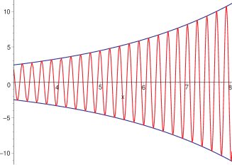
Figure 1: Schematic representation of the coordinate dependence of the neutrino wave packet (16) (arbitrary units).

Having found the expression for the neutrino wave function, we can now calculate the expectation value $\bar{x}$ of the neutrino coordinate as well as the coordinate dispersion, which gives the spatial width of the neutrino wave packet $\sigma_{x\nu}$. In the limit $\Gamma l_{p}/v_{\pi}\gg 1$, when the length of the decay tunnel $l_{p}$ is large compared to the pion decay length $l_{\rm decay}=v_{\pi}/\Gamma$, we find

$$\bar{x}\approx v_{j}t-\frac{v_{j}-v_{\pi}}{\Gamma}\,,\qquad\sigma_{x\nu}\approx\frac{v_{j}-v_{\pi}}{\Gamma}\,.$$ (20)

Note that in this limit the box function in eqs. (16) and (19) has to be replaced by $\theta(v_{j}t-x)$, where $\theta(x)$ is the Heaviside step function.

In the opposite limit, $\Gamma l_{p}/v_{\pi}\ll 1$, we find

$$\bar{x}\approx v_{j}t-\frac{v_{j}-v_{\pi}}{2v_{\pi}}l_{p}\,,\qquad\sigma_{x\nu}\approx\frac{1}{2\sqrt{3}}\frac{v_{j}-v_{\pi}}{v_{\pi}}l_{p}\,.$$ (21)

Notice that in this limit only a small fraction of pions decays before being absorbed by the wall at the end of the decay tunnel.

Although, as was mentioned above, the distance between the sharp borders of the neutrino wave packet is $[(v_{j}-v_{\pi})/v_{\pi}]l_{p}$, the effective spatial width $\sigma_{x\nu}$ of the wave packet is not necessarily determined by this quantity: this is only the case when the exponential decrease of the envelope function is relatively slow, $\Gamma l_{p}/v_{\pi}\ll 1$ (see (21)). In the opposite case, $\Gamma l_{p}/v_{\pi}\gg 1$, which corresponds to the decay of unconfined free pions, it is this exponential decrease that dominates $\sigma_{x\nu}$, as described by eq. (20). It is interesting that the neutrino wave packets are of macroscopic size in the case we consider.

Next, we have to find the amplitude ${\cal A}_{j}(L,t)$ which is the contribution of the $j$th neutrino mass eigenstate to the transition amplitude ${\cal A}_{\alpha\beta}(L,t)$. In the coordinate-space calculation it is simply given by the projection of $\psi_{j}^{S}(x,t)$ onto the detected neutrino state $\psi_{j}^{D}(x)$:

$${\cal A}_{j}(L,t)\equiv\int dx\,\psi_{j}^{D*}(x)\,\psi_{j}^{S}(x,t)\,.$$ (22)

The detected state is in general a wave packet centered on the point $x=L$. In what follows we will be assuming that the detection process is well localized both in space and time, so that the wave function of the detected neutrino state can be represented in the configuration space by $\delta(x-L)$. This requires some explanations. The momentum-space wave function of the detected neutrino state $f_{j}^{D}(p)$ is given by a formula similar to that in eq. (12), with the integration over the detection coordinate $(t^{\prime},\,x^{\prime})$. We assume that the detection process is perfectly localized in space and time, so that the integrand of this formula contains the factor $\delta(x^{\prime}-x_{D})\delta(t^{\prime}-t_{D})$. As a result, $f_{j}^{D}(p)$ is actually momentum independent, and for the coordinate-space wave function of the detected neutrino state centered on the point $x=L$, which is a time-independent Fourier transform of $f_{j}^{D}(p)$ [4, 8], we find $\psi_{j}^{D}(x)=\delta(x-L)$. From (22) we then obtain

$${\cal A}_{j}(L,t)=\psi_{j}^{S}(L,t)\,.$$ (23)

The oscillation probability $P_{\alpha\beta}(L)$ is given, up to a normalization factor, by (see, e.g., [4])

$$P_{\alpha\beta}(L)=\sum_{j,k}U^{*}_{\alpha j}U_{\beta j}U_{\alpha k}U_{\beta k}^{*}\,I_{jk}(L)\,,$$ (24)

where

$$I_{jk}(L)\equiv\int_{-\infty}^{\infty}dt\,{\cal A}_{j}(L,t){\cal A}_{k}^{*}(L,t)\,.$$ (25)

From eq. (23) we then find

$$I_{jk}(L)=\int_{-\infty}^{\infty}\!dt\,\psi_{j}^{S}(L,t)\psi_{k}^{S*}(L,t)\,.$$ (26)

Substituting here the expressions for $\psi_{j}^{S}(x)$ and $\psi_{k}^{S}(x)$ from (16) and performing the integration, we obtain

$$I_{jk}(L)=C_{1}\cdot\frac{i\Gamma}{v_{\pi}\frac{\Delta m_{jk}^{2}}{2P}+i\Gamma}\left[e^{-i\frac{\Delta m_{jk}^{2}}{2P}L}-e^{-\Gamma l_{p}/v_{\pi}}e^{-i\frac{\Delta m_{jk}^{2}}{2P}(L-l_{p})}\right].$$ (27)

Here we have discarded terms $\sim(\Delta m_{jk}^{2})^{2}$ and $\sim\Delta m_{jk}^{2}\Gamma/P$ and neglected the difference between $v_{j}$ and $v_{k}$ whenever they are multiplied by $\Gamma$ or by $\Delta m^{2}/2P$. The constant $C_{1}$ can be found by imposing the unitarity constraint $\sum_{\beta}P_{\alpha\beta}(L)=1$ on the oscillation probability (24), which leads to the normalization condition $I_{jj}(L)=1$ [4]. This yields $C_{1}=(1-e^{-\Gamma l_{p}/v_{\pi}})^{-1}$, so that we finally obtain

$$I_{jk}(L)=\frac{1}{(1-e^{-\Gamma l_{p}/v_{\pi}})}\cdot\frac{i\Gamma}{v_{\pi}\frac{\Delta m_{jk}^{2}}{2P}+i\Gamma}\left[e^{-i\frac{\Delta m_{jk}^{2}}{2P}L}-e^{-\Gamma l_{p}/v_{\pi}}e^{-i\frac{\Delta m_{jk}^{2}}{2P}(L-l_{p})}\right].$$ (28)

By making use of the normalization condition $I_{jj}(L)=1$ one can demonstrate that the quantity $I_{jk}(L)$ (and therefore the oscillation probability (24)) is Lorentz invariant [4].

2.4 The oscillation probability

With the expression for $I_{jk}(L)$ at hand, we can now calculate the oscillation probabilities from eq. (24). Consider a 2-flavour case when the oscillations are governed by just one mass squared difference and one mixing angle. As an example, short-baseline oscillations in the 3+1 scheme with one sterile neutrino are essentially reduced to effective 2-flavour ones with $\Delta m^{2}\equiv\Delta m_{41}^{2}\neq 0$, while the much smaller mass squared differences $\Delta m_{31}^{2}$ and $\Delta m_{21}^{2}$ can be neglected. In this case the survival probabilities $P_{\alpha\alpha}$ are described by the effective mixing parameters

$$\sin\theta\equiv s=|U_{\alpha 4}|\,,\qquad\quad\cos\theta\equiv c=(1-|U_{\alpha 4}|^{2})^{1/2}\,.$$ (29)

In the case of transition probabilities $P_{\alpha\beta}$ ($\alpha\neq\beta$), the mixing parameter can be chosen as

$$\sin^{2}2\theta\equiv 4|U_{\alpha 4}|^{2}|U_{\beta 4}|^{2}\,.$$ (30)

Consider, for example, the survival probability of muon neutrinos in the 2-flavour scheme. From eqs. (24) and (28) we find

$$P_{\mu\mu}=c^{4}+s^{4}+\frac{2c^{2}s^{2}}{\xi^{2}+1}\frac{1}{(1-e^{-\Gamma l_{p}/v_{\pi}})}\left[\cos\phi+\xi\sin\phi-e^{-\Gamma l_{p}/v_{\pi}}[\cos(\phi-\phi_{p})+\xi\sin(\phi-\phi_{p})]\right].$$ (31)

Here

$$\phi\equiv\frac{\Delta m^{2}}{2P}L\,,\qquad\phi_{p}\equiv\frac{\Delta m^{2}}{2P}l_{p}\,,$$ (32)

and we have defined the parameter

$$\xi\equiv v_{\pi}\frac{\Delta m^{2}}{2P\Gamma}\,,$$ (33)

which, along with $\Gamma l_{p}/v_{\pi}$, characterizes possible decoherence effects at neutrino production (see the discussion in section 2.5). In the limit $v_{\pi}=1$ eq. (31) coincides with result found in ref. [3].

We shall now analyze the probability (31) in the light of neutrino production coherence.

2.5 Coherence violation at neutrino production

Let us start with a qualitative analysis of neutrino production coherence. Recall that the production coherence condition requires that different neutrino mass eigenstates forming a flavor neutrino state be emitted coherently in the production process. This condition can be written as

$$\Delta E\ll\sigma_{E}\,,$$ (34)

where $\Delta E$ is the energy difference of different neutrino mass eigenstates and $\sigma_{E}$ is the quantum-mechanical energy uncertainty inherent to the production process. As was pointed out in [4], for decays of non-relativistic parent particles contained in a box of finite size, $\sigma_{E}$ is determined by the larger of the two quantities: the particle’s decay width $\Gamma$ and the inverse time between two subsequent collisions of the particle with the walls of the box. In our case, the “collision time” is the time $l_{p}/v_{\pi}$ between the pion production and absorption of undecayed pions at the end of the decay tunnel. In general, for relativistic parent particles of velocity $v_{P}$ this non-relativistic energy uncertainty should be multiplied by the factor $v_{g}/(v_{g}-v_{P})$. This takes into account that the neutrino is emitted by a moving particle in the forward direction, so that the parent particle “chases” the produced neutrino wave packet [12, 4]. We thus find that in our case

$$\sigma_{E}\sim\max\{\Gamma,v_{\pi}/l_{p}\}\frac{v_{g}}{v_{g}-v_{\pi}}\,.$$ (35)

It is known that the energy uncertainty $\sigma_{E}$ also determines the spatial width of the neutrino wave packet [4]: $\sigma_{x\nu}\simeq v_{g}/\sigma_{E}$. From (35) we therefore find that in the limiting case $\Gamma l_{p}/v_{\pi}\gg 1$ the width of the wave packet $\sigma_{x\nu}\sim(v_{g}-v_{\pi})/\Gamma$, whereas for $\Gamma l_{p}/v_{\pi}\ll 1$ one finds $\sigma_{x\nu}\sim[(v_{g}-v_{\pi})/v_{\pi}]l_{p}$. These results are in full accord with our previously found values of $\sigma_{x\nu}$ (see eqs. (20) and (21)).

As follows from (18),

$$\Delta E\equiv|E_{j}(P_{j})-E_{k}(P_{k})|\simeq\frac{\Delta m^{2}}{2P}\frac{v_{\pi}v_{g}}{(v_{g}-v_{\pi})}\,.$$ (36)

Taking into account eq. (35), for the (de)coherence parameter $\Delta E/\sigma_{E}$ we then find

$$\frac{\Delta E}{\sigma_{E}}\simeq\frac{\Delta m^{2}}{2P}l_{p}=\phi_{p}\,,\quad(\Gamma l_{p}/v_{\pi}\ll 1)\,;\qquad\qquad\frac{\Delta E}{\sigma_{E}}\simeq\xi\quad(\Gamma l_{p}/v_{\pi}\gg 1)\,.$$ (37)

Let us now consider the probability (31) from the point of view of the production decoherence effects (see also [3]). As was mentioned above, these effects depend in general on two parameters, $\xi$ and $\Gamma l_{p}/v_{\pi}$. Note that these quantities have different dependence on the pion lifetime $\Gamma$, and that there is a relation between them and the phase $\phi_{p}$:

$$\xi\cdot\frac{\Gamma l_{p}}{v_{\pi}}=\phi_{p}\,.$$ (38)

The three quantities in this equation can also be expressed through the pion decay length $l_{\rm decay}=v_{\pi}/\Gamma$ and the neutrino oscillation length $l_{\rm osc}=4\pi P/\Delta m^{2}$:

$$\xi=2\pi\frac{l_{\rm decay}}{l_{\rm osc}}\,,\qquad\quad\frac{\Gamma l_{p}}{v_{\pi}}=\frac{l_{p}}{l_{\rm decay}}\,,\qquad\quad\phi_{p}=2\pi\frac{l_{p}}{l_{\rm osc}}\,.$$ (39)

Consider first the limit $\Gamma l_{p}/v_{\pi}\ll 1$. As follows from (37), the decoherence parameter in this case is $\phi_{p}$. Thus, one can expect strong decoherence effects for $\phi_{p}\gg 1$ and no decoherence in the opposite limit.

The case $\Gamma l_{p}/v_{\pi}\ll 1$ is actually more easily studied by going to this limit in the expression for $I_{jk}(L)$ and then calculating the oscillation probabilities rather than by directly expanding the expressions for oscillation probabilities. Taking the limit $\Gamma l_{p}/v_{\pi}\ll 1$ in (28), we obtain

$$I_{jk}(L)=\frac{i}{\frac{\Delta m_{jk}^{2}}{2P}l_{p}}\left[e^{-i\frac{\Delta m_{jk}^{2}}{2P}L}-e^{-i\frac{\Delta m_{jk}^{2}}{2P}(L-l_{p})}\right].$$ (40)

Note that this quantity satisfies the correct normalization condition $I_{jj}(L)=1$ provided that $\Delta m_{jj}^{2}$ is understood as the limit $\Delta m_{jk}^{2}\to 0$. Substituting (40) into (24), we find

$$P_{\mu\mu}=c^{4}+s^{4}+\frac{2s^{2}c^{2}}{\phi_{p}}\big{[}\sin\phi-\sin(\phi-\phi_{p})\big{]}\,.$$ (41)

In the limit $\phi_{p}\gg 1$ this expression yields $P_{\mu\mu}\simeq c^{4}+s^{4}$, which corresponds to averaged neutrino oscillations, whereas for $\phi_{p}\ll 1$ it gives the standard oscillation probability

$$P^{\rm stand}_{\mu\mu}=c^{4}+s^{4}+2s^{2}c^{2}\cos\phi\,,$$ (42)

as expected. Let us stress that the latter result does not depend on whether $\xi$ is small or large, though $\xi$ must still satisfy the relation in eq. (38). As follows from the same relation, in the case $\phi_{p}\gg 1$ (strong decoherence) $\xi$ is automatically very large in the $\Gamma l_{p}/v_{\pi}\ll 1$ regime.

Consider now the limit $\Gamma l_{p}/v_{\pi}\gg 1$, when most pions decay before reaching the end of the decay tunnel. In this case, according to (37), decoherence effects should be governed by the parameter $\xi$. As expected, in the limit $\xi\to 0$ eq. (31) yields the standard oscillation probability (42), whereas for $\xi\gg 1$ the oscillating terms in (31) are suppressed and one obtains the averaged probability $P_{\mu\mu}\simeq c^{4}+s^{4}$.

Thus, we conclude that in the case of sufficiently small $l_{p}$, when both $\Gamma l_{p}/v_{\pi}\ll 1$ and $\phi_{p}\ll 1$, the production coherence condition is always satisfied (and the oscillation probability takes its standard form) irrespective of the value of $\xi$, which is irrelevant in this case. If $\Gamma l_{p}/v_{\pi}\ll 1$ but $\phi_{p}\gtrsim 1$ (which implies $l_{\rm osc}/2\pi\lesssim l_{p}\ll l_{\rm decay}$), the production coherence is moderately or strongly violated, depending on the value of $\phi_{p}$. In the case $\Gamma l_{p}/v_{\pi}\gg 1$ the production coherence depends on the parameter $\xi$: it is satisfied for $\xi\ll 1$ and strongly violated in the opposite case.

Irrespectively of the value of $\Gamma l_{p}/v_{\pi}$, strong production coherence violation always implies $\xi\gg 1$, although large values of $\xi$ do not necessarily imply coherence violation. It is easy to see that the same applies to $\phi_{p}$. Therefore, in order to find out if the production coherence is violated one has to check the values of any two out of the three parameters $\Gamma l_{p}/v_{\pi}$, $\xi$ and $\phi_{p}$ (the third one will then be given by eq. (38)). It is convenient to choose these to be $\xi$ and $\phi_{p}$.

Indeed, from the above considerations it is easy to see that if $\Gamma l_{p}/v_{\pi}$ is very small or very large, the production coherence is strongly violated in the case $\xi\gg 1$, $\phi_{p}\gg 1$ and is satisfied in all other limiting cases (large $\xi$ and small $\phi_{p}$, small $\xi$ and large $\phi_{p}$, and small $\xi$, small $\phi_{p}$). If $\Gamma l_{p}/v_{\pi}\sim 1$, the parameters $\xi$ and $\phi_{p}$ in the limiting cases are either both small or both large, and from eq. (31) it again follows that the production coherence is strongly violated if $\xi\gg 1$, $\phi_{p}\gg 1$. It is satisfied in the opposite case.

In the intermediate cases one can expect moderate violation of the production coherence, which should lead to noticeable deviations of the oscillation probabilities from their standard (i.e. predicted under the coherence assumption) values.

3 Incoherent probability summation approach

Let us now consider oscillations of neutrinos produced in pion decays inside a decay tunnel in a entirely different approach [3]. We will be assuming that each individual neutrino production event is completely coherent, so that the oscillations of the produced neutrino are described by the standard probability (42). At the same time, one has to take into account that the neutrino production can take place at any point along the decay tunnel, though the pion flux decreases exponentially with the distance from the pion production point. The oscillated neutrino flux at a detector at the distance $L$ from the beginning of the tunnel is then given by

$$F_{\mu}(E,L)\,=\,F_{\pi}(E,0)\Gamma\int_{0}^{l_{p}}e^{-\frac{\Gamma x}{v_{\pi}}}\,P^{\rm stand}_{\mu\mu}(E,L-x)dx\,,$$ (43)

where $F_{\pi}(E,0)$ is the initially produced pion flux. The unoscillated neutrino flux $F_{\mu}^{0}$ (i.e. the $\nu_{\mu}$ flux in the absence of the oscillations) is given by eq. (43) with $P^{\rm stand}_{\mu\mu}(E,L-x)$ in the integrand replaced by 1. One can now define the effective oscillation probability as the ratio of the oscillated and unoscillated fluxes:

$$P^{\rm eff}_{\mu\mu}(L,E)\;\equiv\;F_{\mu}(L,E)/F_{\mu}^{0}(L,E)\,.$$ (44)

The calculation is straightforward, and the result turns out to coincide exactly with the expression for $P_{\mu\mu}(E,L)$ given by eq. (31). Thus, the summation of the amplitudes of neutrino production at different points along the pion path performed in section 2 and the summation of the corresponding probabilities carried out in this section lead to the same oscillation probability. We will discuss the reason for this intriguing coincidence and the conditions under which it is broken in section 6 and in the Discussion section.

4 Amplitude summation: The case of finite-width pion wave packets

Let us now relax the assumption of pointlike pions that we employed in section 2. For the pion wave function we will use the expression similar to (9), but with $\delta(x-v_{\pi}t)$ replaced by a general shape factor $g_{\pi}(x-v_{\pi}t)$:

$$\psi_{\pi}(x,t)=C_{\pi}\,e^{iQx-iE_{\pi}(Q)t-\Gamma t/2}\,g_{\pi}(x-v_{\pi}t)\,{\rm box}(x;l_{p},0)\,.$$ (45)

We will be assuming that $g_{\pi}(x-v_{\pi}t)$ is peaked at or near the zero of its argument and rapidly decreases when $|x-v_{\pi}t|\gtrsim\sigma_{x\pi}$, but otherwise will not specify the exact form of this function. Substituting (45) into (12), for the momentum-space wave packet of the $j$th mass eigenstate component of the produced neutrino we obtain

$$f_{j}^{S}(p)=M_{P}C_{\pi}\int_{0}^{l_{p}}dx\,e^{i[E_{j}(p)-E_{P}]\frac{x}{v_{\pi}}-i(p-P)x-\frac{\Gamma}{2v_{\pi}}x}\;\bar{g}_{\pi}(E_{j}(p)-E_{P})\,,$$ (46)

where $\bar{g}_{\pi}(E_{j}(p)-E_{P})$ is the Fourier transform of $g_{\pi}(x-v_{\pi}t)\,e^{-\frac{\Gamma}{2v_{\pi}}(v_{\pi}t-x)}$:

$$\bar{g}_{\pi}(E_{j}(p)-E_{P})=\int_{-\infty}^{\infty}dt^{\prime}\,e^{i[E_{j}(p)-E_{P}]t^{\prime}}\,[g_{\pi}(-v_{\pi}t^{\prime})e^{-\frac{\Gamma}{2}t^{\prime}}]\,.$$ (47)

Here the integration variable is $t^{\prime}=t-x/v_{\pi}$. Note that the integration has been extended to the negative semi-axis of $t^{\prime}$ here; this is justified only if for large negative $t^{\prime}$ the function $g_{\pi}(-v_{\pi}t^{\prime})$ decreases sufficiently rapidly, and in any case faster than $e^{-\Gamma|t^{\prime}|/2}$. This condition is satisfied for both box-type and Gaussian pion wave packets which we will consider below.

Performing the integration over $x$ in (46), we obtain

$$f_{j}^{S}(p)=C_{j}\frac{1-e^{i[E_{j}(p)-E_{P}-v_{\pi}(p-P)+i\frac{\Gamma}{2}]\frac{l_{p}}{v_{\pi}}}}{E_{j}(p)-E_{P}-v_{\pi}(p-P)+i\frac{\Gamma}{2}}\,\bar{g}_{\pi}(E_{j}(p)-E_{P})\,,$$ (48)

where $C_{j}$ is a constant. This expression differs from the corresponding one in the case of pointlike pions (13) by the extra factor $\bar{g}_{\pi}(E_{j}(p)-E_{P})$.

Let us now calculate the transition amplitude and the quantity $I_{jk}(L)$. We will be again assuming that the detection process is well localized in space and time. The contribution of the $j$th neutrino mass eigenstates to the oscillation amplitude is then given, according to eqs. (23) and (15), by

$${\cal A}_{j}(L,t)=\int\frac{dp}{2\pi}f_{j}^{S}(p)e^{ipL-iE_{j}(p)t}\,.$$ (49)

Substituting this into eq. (25) and performing the integration over $t$, we find

$$I_{jk}(L)=\int\frac{dp_{1}dp_{2}}{(2\pi)^{2}}\,f_{j}^{S}(p_{1})f_{k}^{S*}(p_{2})\,e^{i(p_{1}-p_{2})L}\,2\pi\delta[E_{j}(p_{1})-E_{k}(p_{2})]$$

$$=e^{-i\frac{\Delta m_{jk}^{2}}{2P}L}\,\frac{1}{v_{g}}\int\frac{dp_{1}}{2\pi}\,f_{j}^{S}(p_{1})f_{k}^{S*}(p_{1}+\Delta m_{jk}^{2}/2P)\,.$$ (50)

Here we have used

$$\delta[E_{j}(p_{1})-E_{k}(p_{2})]\simeq\delta[v_{g}(p_{1}-p_{2})+\Delta m_{jk}^{2}/2E]\,,$$ (51)

which follows from $E_{j}(p_{1})-E_{k}(p_{2})\simeq(\partial E/\partial p)\Delta p+(\partial E/\partial m^{2})\Delta m^{2}$. Substituting (48) into (50), we obtain

$$I_{jk}(L) =\frac{C_{j}C_{k}^{*}}{v_{g}^{2}}\,e^{-i\frac{\Delta m_{jk}^{2}}{2P}L}\,\int\frac{dp}{2\pi}\,\frac{[1-e^{i[E_{j}(p)-E_{P}-v_{\pi}(p-P)+i\frac{\Gamma}{2}]\frac{l_{p}}{v_{\pi}}}]\bar{g}_{\pi}(E_{j}(p)-E_{P})}{E_{j}(p)-E_{P}-v_{\pi}(p-P)+i\frac{\Gamma}{2}}\vspace*{2.5mm}\qquad$$

$$\times\frac{[1-e^{-i[E_{k}(p+\Delta m_{jk}^{2}/2P)-E_{P}-v_{\pi}(p+\Delta m_{jk}^{2}/2P-P)-i\frac{\Gamma}{2}]\frac{l_{p}}{v_{\pi}}}]\bar{g}_{\pi}^{*}\big{(}E_{k}\big{(}p+\frac{\Delta m_{jk}^{2}}{2P}\big{)}-E_{P}\big{)}}{E_{k}\big{(}p+\frac{\Delta m_{jk}^{2}}{2P}\big{)}-E_{P}-v_{\pi}\big{(}p+\frac{\Delta m_{jk}^{2}}{2P}-P\big{)}-i\frac{\Gamma}{2}}\,.$$ (52)

As usual, the constant $C_{j}$ should be found from the condition $I_{jj}(L)=1$.

We shall now consider two special cases, Gaussian and box-type pion wave packets.

4.1 Gaussian shape factor of the pion wave packet

In this case

$$g_{\pi}(x-v_{\pi}t)=e^{-\frac{(x-v_{\pi}t)^{2}}{4\sigma_{x\pi}^{2}}}\,,$$ (53)

which gives

$$\bar{g}(E_{j}(p)-E_{P})=const.\,e^{-\frac{\sigma_{x\pi}^{2}}{v_{\pi}^{2}}[E_{j}(p)-E_{P}+i\frac{\Gamma}{2}]^{2}}\,.$$ (54)

Let us calculate $I_{jk}(L)$ in the limit $\Gamma l_{p}/v_{\pi}\gg 1$, which corresponds to the situation when most pions decay before they reach the end of the decay tunnel. Substituting (54) into (52) and expanding $E_{j}(p)$ near the point $p=P$ up to terms linear in $p-P$, we find

$$I_{jk}(L)=C_{jk}\frac{e^{-i\frac{\Delta m_{jk}^{2}}{2P}L}}{1-i\xi}\Big{\{}e^{2\sigma_{x\pi}^{2}\Big{(}\frac{\Gamma}{2(v_{g}-v_{\pi})}\frac{v_{g}}{v_{\pi}}+iB_{j}\Big{)}^{2}}{\rm erfc}\Big{[}\sqrt{2}\sigma_{x\pi}\Big{(}\frac{\Gamma}{2(v_{g}-v_{\pi})}\frac{v_{g}}{v_{\pi}}+iB_{j}\Big{)}\Big{]}$$

$$+e^{2\sigma_{x\pi}^{2}\Big{(}\frac{v_{g}}{v_{\pi}}\frac{\Gamma}{2(v_{g}-v_{\pi})}-iB_{k}\Big{)}^{2}}{\rm erfc}\Big{[}\sqrt{2}\sigma_{x\pi}\Big{(}\frac{\Gamma}{2(v_{g}-v_{\pi})}\frac{v_{g}}{v_{\pi}}-iB_{k}\Big{)}\Big{]}\Big{\}}\,,$$ (55)

where ${\rm erfc(z)}$ is the complementary error function, the constant $C_{jk}\propto C_{j}C_{k}^{*}$ is fixed by the condition $I_{jj}(L)=1$, and

$$B_{j}\equiv\frac{E_{P}-E_{j}(P)}{v_{j}-v_{\pi}}\,.$$ (56)

The oscillation probabilities can now be obtained from eq. (24). We will consider the limit of small $\sigma_{x\pi}$, in which the result simplifies considerably. In the lowest non-trivial order in this parameter we obtain, after the proper normalization,

$$I_{jk}(L)=\frac{e^{-i\frac{\Delta m_{jk}^{2}}{2P}L}}{1-i\xi}\Big{[}1+i\frac{2}{\sqrt{2\pi}}\,\frac{v_{g}}{v_{g}-v_{\pi}}\,\frac{\Delta m_{jk}^{2}}{2P}\,\sigma_{x\pi}\Big{]}\,.$$ (57)

For the $\nu_{\mu}$ survival probability we then find

$$P_{\mu\mu}=c^{4}+s^{4}+\frac{2c^{2}s^{2}}{\xi^{2}+1}\left[(\cos\phi+\xi\sin\phi)-A_{\pi}(\xi\cos\phi-\sin\phi)\right]\,,$$ (58)

where

$$A_{\pi}=A_{\pi\rm Gauss}=\frac{2}{\sqrt{2\pi}}\,\frac{v_{g}}{v_{g}-v_{\pi}}\,\frac{\Delta m_{jk}^{2}}{2P}\,\sigma_{x\pi}\,.$$ (59)

The term independent of $\sigma_{x\pi}$ here coincides with the $\Gamma l_{p}/v_{\pi}\gg 1$ limit of the $\nu_{\mu}$ survival probability (31) obtained in the case of neutrinos produced in decays of pointlike pions, whereas the term proportional to $A_{\pi}$ gives the correction due to the finite size of the pion wave packets. Note that eq. (58) is actually the expansion of

$$P_{\mu\mu}=c^{4}+s^{4}+\frac{2c^{2}s^{2}}{\xi^{2}+1}\left[\cos(\phi-A_{\pi})+\xi\sin(\phi-A_{\pi})\right]\,,$$ (60)

to the lowest non-trivial order in $A_{\pi}$, which shows that to this order the effect of the finite-size pion wave packets reduces to an additional oscillation phase proportional to $\sigma_{x\pi}$.

4.2 Box-type shape factor of the pion wave packet

Consider now a box-type shape factor for the pion wave packet:

$$g_{\pi}(x-v_{\pi}t)=box(v_{\pi}t-x,d,0)\,.$$ (61)

It corresponds to the pion wave packet of width $d$ and the initial condition that the pion starts arriving in the decay tunnel at $t=0$. From (47) we have

$$\bar{g}_{\pi}(E_{j}(p)-E_{P})=i\,\frac{1-e^{i[E_{j}(p)-E_{P}+i\frac{\Gamma}{2}]\frac{d}{v_{\pi}}}}{E_{j}(p)-E_{P}+i\frac{\Gamma}{2}}\,.$$ (62)

To facilitate comparison with the Gaussian pion wave packet case, it will be convenient for us to express the parameter $d$ through the effective spatial width of the pion wave packet $\sigma_{x\pi}$. The latter we always define as the coordinate dispersion in a given state, $[\langle x^{2}\rangle-\langle x\rangle^{2}]^{1/2}$. For the pion state (61) we thus find

$$\sigma_{x\pi}=\frac{d}{2\sqrt{3}}\,.$$ (63)

Consider once again the limit $\Gamma l_{p}/v_{\pi}\gg 1$. Substituting (62) into (52) gives, in the leading non-trivial order in $\sigma_{x\pi}$,

$$I_{jk}(L)=\frac{e^{-i\frac{\Delta m_{jk}^{2}}{2P}L}}{1-i\xi}\Big{[}1+i\frac{1}{\sqrt{3}}\,\frac{v_{g}}{v_{g}-v_{\pi}}\,\frac{\Delta m_{jk}^{2}}{2P}\,\sigma_{x\pi}\Big{]}\,.$$ (64)

The probability $P_{\mu\mu}$ is then again given by eq. (58) but now with

$$A_{\pi}=A_{\pi\rm box}=\frac{1}{\sqrt{3}}\,\frac{v_{g}}{v_{g}-v_{\pi}}\,\frac{\Delta m_{jk}^{2}}{2P}\,\sigma_{x\pi}\,.$$ (65)

Comparing eqs. (57) and (64) we see that they have the same structure: there is a term of the zeroth order in $\sigma_{x\pi}$ which coincides with the corresponding expression in the $\Gamma l_{p}/v_{\pi}\gg 1$ limit of the case of pointlike pions (see eq. (28)), and the term which is linear in $\sigma_{x\pi}$. The coefficients in front of $\sigma_{x\pi}$ in the cases of box-type and Gaussian type pion wave packets differ only by a numerical factor. The same applies to the expression for $P_{\mu\mu}$ – in both cases it is given by the same eq. (58) with the coefficients $A_{\pi}$ only differing by a numerical factor. Note that expressions (57), (64) and (58) were obtained in the limit of small $A_{\pi}$ and therefore cannot describe neutrino production decoherence caused by the finite size of the pion wave packet (which would correspond to $A_{\pi}\gtrsim 1$); they just describe the appearance of extra oscillatory terms in the transition and survival probabilities rather than suppression of such terms. We will consider the decoherence effects due to $\sigma_{x\pi}\neq 0$ in section 6.2. For now, we will explain qualitatively the structure of the order $\sigma_{x\pi}$ correction term in the oscillation probability (58) and in particular its proportionality to $v_{g}/(v_{g}-v_{\pi})$.

4.3 Small corrections due to $\sigma_{x\pi}\neq 0$: a qualitative analysis

If the pion wave packet has a finite spatial width, there is a an additional contribution $\Delta\phi$ to the oscillation phase stemming from the fact that the neutrino production region (and the space-time interval of integration over the neutrino production coordinate) is different in this case. One has therefore to add $\Delta\phi$ to the oscillation phase $\phi$ corresponding to the case of pointlike pions.

Neutrino emission in a decay of an extended pion is schematically illustrated in fig. 2. The wave packet of the pion is represented by a band in the $(t,x)$ plane, the muon wave packet is not shown. The slanted line represents the neutrino trajectory corresponding to the exact space and time localization of its detection. For neutrino emission from the space-time point $A$ the additional oscillation phase as compared to neutrino emitted from the point $B$ is given by the difference of the phases acquired by the mass eigenstates $\nu_{j}$ and $\nu_{k}$ along the segment $AB$ shown in the figure:

$$\Delta\phi=-[E_{j}(P_{j})-E_{k}(P_{k})]\Delta t+(P_{j}-P_{k})\Delta x\,.$$ (66)

The quantities $\Delta t$ and $\Delta x$ are given by the projections of the segment $AB$ on the $t$ and $x$ axes. Simple geometric considerations yield

$$\Delta t=\frac{\sigma_{x\pi}}{v_{g}-v_{\pi}}\,,\qquad\quad\Delta x=\sigma_{x\pi}\frac{v_{g}}{v_{g}-v_{\pi}}\,.$$ (67)

Substituting (67) into (66) and using eqs. (17) and (18), we find

$$\Delta\phi\simeq-\frac{v_{g}}{v_{g}-v_{\pi}}\!\cdot\!\frac{\Delta m_{jk}^{2}}{2P}\sigma_{x\pi}\,.$$ (68)

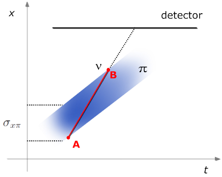
Figure 2: Schematical illustration of neutrino emission in pion decay in the case of finite-width pion wave packets.

This quantity does not depend on $t_{A}$ and therefore the same additional phase appears for neutrinos emitted at any time. The quantity $I_{jk}(L)$ can now be obtained from the one in the case of pointlike pions (eq. (28)) by substituting $\phi\to\phi+\Delta\phi$. Taking the limit $\Gamma l_{p}/v_{\pi}\gg 1$ and keeping only the terms up to the first power in $\Delta\phi$, for the probability $P_{\mu\mu}$ we then obtain eq. (58) with $A_{\pi}=-\Delta\phi$ (cf. eqs. (58) and (60)). The correction to the oscillation probability due to $\sigma_{x\pi}\neq 0$ obtained here from simple qualitative considerations coincides, up to numerical factors of order one, with those found in the previous subsections for the Gaussian and box-type pion wave packets. The exact value of the numerical coefficient depends on the shape of the pion wave packet.

5 Probability summation and finite-thickness targets

We shall now study the case when a proton beam is incident on a target of finite thickness and will treat this case in the framework of incoherent probability summation. This procedure is just the one that is usually employed in the analyses of neutrino oscillation experiments in order to take into account the extended sizes of neutrino sources (and detectors). The results of this section will also turn out to be useful for comparing the probability summation approach with the coherent amplitude summation in the case of finite widths of the pion wave packets. We therefore examine this case in detail.

Consider a bunch of protons of duration $t_{bunch}$ with certain time distribution of protons within the bunch corresponding to a flux density $F_{p}(t)$. The protons are incident on a target of width $D$ and density distribution $n_{tar}(x)$ which in general depends on the coordinate $x$ along the direction of the beam. We assume that the protons produce pions on different scatterers incoherently. Consider the situation when the time of the pion production as well as the time of neutrino detection are not measured and the neutrino signal is summed up over the bunch. The total number of pions produced in the layer $(x,\,x+dx)$ of the target by the proton bunch is

$$dn_{\pi}(x)=k_{\pi}\int dt\,A(x)F_{p}(t)\,\sigma\,n_{tar}(x)dx=k_{\pi}\sigma F_{p}^{int}A(x)n_{tar}(x)dx\,,$$ (69)

where $\sigma$ is the $pN-$cross-section, $A(x)$ is the factor describing the attenuation of the proton beam in the target by the time it reaches the point with the coordinate $x$, $k_{\pi}$ is the average number of pions produced in each interaction, and

$$F_{p}^{int}\equiv\int dtF_{p}(t)$$ (70)

is the integral proton flux. Notice that at this point the time dependence factorizes out and disappears from the whole picture: obviously, the obtained result does not depend on a specific time dependence of the proton flux.

The number of muon neutrinos at the detector which originate from the decays of pions born in the layer $(x,x+dx)$ of the target can be written as

$$dn_{\pi}(x)\int_{x}^{l_{p}}dx^{\prime}e^{-\frac{\Gamma}{v_{\pi}}(x^{\prime}-x)}P^{\rm stand}_{\mu\mu}(L-x^{\prime})\,.$$ (71)

Here $x^{\prime}$ is the distance from the front end of the target (from the side of the incoming proton beam) to the point of the pion decay, $L$ is the distance from the target’s front end to the detector, and $P^{\rm stand}_{\mu\mu}(L-x)$ is given by eqs. (42) and (32) with $L$ replaced by $L-x$. The total number of muon neutrinos at the detector site, which originate from the decays of pions produced over the whole target, is

$$N_{\nu}=\sigma F_{p}^{int}k_{\pi}\int_{0}^{D}dz\,n_{tar}(z)A(z)\int_{z}^{l_{p}}dxe^{-\frac{\Gamma}{v_{\pi}}(x-z)}P_{\mu\mu}^{\rm stand}(L-x)\,.$$ (72)

Let us consider some special limits of this expression.

1. Very thin target:

$$n_{tar}(z)=n_{0}\delta(z),~{}~{}~{}A(0)=1.$$ (73)

In this case

$$N_{\nu}=F_{p}^{int}k_{\pi}n_{0}\int_{0}^{l_{p}}dxe^{-\frac{\Gamma}{v_{\pi}}x}P_{\mu\mu}^{\rm stand}(L-x)\,,$$ (74)

and the integration leads to the effective oscillation probability $P_{\mu\mu}$ that coincides with the one in eq. (31) (see (43)).

2. Short decay tunnel: $l_{p}\ll v_{\pi}/\Gamma$. In this case

$$N_{\nu}\approx F_{p}^{int}k_{\pi}\int_{0}^{D}dz~{}n_{tar}(z)A(z)\int_{z}^{l_{p}}dxP_{\mu\mu}^{\rm stand}(L-x)\,.$$ (75)

Assuming for simplicity that $n_{tar}(z)=n_{tar}=const$ and $A(z)=A_{0}=const$, we find

$$N_{\nu}\approx F_{p}^{int}k_{\pi}n_{tar}A_{0}\int_{0}^{D}dz\int_{z}^{l_{p}}dxP_{\mu\mu}^{\rm stand}(L-x)\,.$$ (76)

Straightforward integration yields

$$P_{\rm eff}\equiv\frac{N_{\nu}}{N_{\nu}^{0}}\approx c^{4}+s^{4}+2c^{2}s^{2}\frac{1}{\phi_{p}}\Big{[}\sin\phi-\sin(\phi-\phi_{p})+\frac{D}{2l_{p}}\left(\sin\phi-\sin(\phi-\phi_{p})\right)-\frac{\pi D}{l_{\rm osc}}\cos\phi\Big{]},$$ (77)

where we have retained only terms up to the first order in $D$. In the limit $D\rightarrow 0$ this expression reduces to the one in eq. (41).

3. Extended target and well localized protons. Assume that the decay tunnel is long, so that $l_{\rm decay}=v_{\pi}/\Gamma\ll l_{p}$. This is the same limit as the one used in the coherent amplitude summation calculations with finite-width pion wave packets carried out in sections 4.1 and 4.2. We also assume that the density of the target is constant and that there is no absorption, i.e. $n_{tar}(z)A(z)=const$. Thus, we have the setup which corresponds to the one that in the amplitude summation approach led to the box-type pion wave packets. From eq. (72) we find

$$N_{\nu}\propto\int_{0}^{D}dz\int_{z}^{L}dxe^{-\frac{\Gamma}{v_{\pi}}(x-z)}P_{\mu\mu}^{\rm stand}(L-x)\,.$$ (78)

The integration yields

$$P_{\rm eff}=\frac{N_{\nu}}{N_{\nu}^{0}}\approx c^{4}+s^{4}+\frac{2c^{2}s^{2}}{1+\xi^{2}}\Big{[}\cos\phi+\xi\sin\phi-\frac{\Delta m^{2}}{4P}D(\xi\cos\phi-\sin\phi)\Big{]},$$ (79)

where only corrections of the first order in $D$ are kept.

Now let us compare the above results with those of the coherent amplitude summation approach with finite spatial width of the pion wave packets.

What could be an analogue of the finite-width pion wave packet in the case when one performs the summation of contributions of neutrino production at different points at the level of probabilities? In that case the standard oscillation probability is used, and the notion of the pion wave packet does not apply. Nonetheless, one can introduce an analogy between the incoherent probability summation approach and the coherent amplitude summation with finite $\sigma_{x\pi}$ in the following way.

In sec. 2, when considering the oscillations of neutrinos produced in pion decays in the amplitude summation approach, we estimated the width of the pion wave packets assuming that the pions are produced by proton collisions with nuclei of a target and that these nuclei are well localized and are essentially pointlike, whereas the protons are described by extended wave packets (see eqs. (6) and (7)). However, one can instead imagine that the protons are pointlike, whereas the nuclei of the target are localized in relatively large spatial region of size $D$, so that their wave packets are characterized by the spatial width $\sigma_{xN}\simeq D$. In this case eqs. (3), (4) and (6) yield $\sigma_{xP}=\sigma_{xp}\approx 0$, $v_{P}\approx v_{p}$, $\sigma_{e\pi}\approx v_{p}/D$, and from eq. (5) we find, instead of (7),

$$\sigma_{x\pi}\simeq\frac{v_{p}-v_{\pi}}{v_{p}}\,D\,.$$ (80)

On the other hand, in the probability summation approach one can identify the spatial size of the localization region of the target nuclei with the extension of the target in the direction of the proton beam. Therefore, when one employs the probability summation approach, the role of an analogue of the finite-size pion wave packets could be played by the finite-thickness target, with the correspondence between the thickness of the target $D$ in the probability summation approach and the width of the pion wave packet $\sigma_{x\pi}$ in the amplitude summation one established by eq. (80). Such a calculation was carried out in example 3 above, and the result is given in eq. (79). Note that the obtained expression for the effective muon neutrino survival probability $P_{\rm eff}$ has the same structure as the probability $P_{\mu\mu}$ in eq. (58), which was derived in the coherent amplitude summation approach in the leading non-trivial order in $\sigma_{x\pi}$. The two expressions, however, differ by the coefficients in front of the second terms in the square brackets: while in the amplitude summation framework with box-type pion wave packets it was given by $A_{\pi{\rm box}}$ of eq. (65), in the probability summation approach of this subsection it is

$$\frac{\Delta m^{2}}{4P}D=\frac{\Delta m^{2}}{4P}\frac{v_{p}}{v_{p}-v_{\pi}}\,\sigma_{x\pi}\,.$$ (81)

Here in the last equality we have used relation (80) which establishes the correspondence between the proton target thickness $D$ of the probability summation approach and the width of the pion wave packet of the amplitude summation one. It is interesting to note that the expressions in eqs. (65) and (81) differ only by the replacement of the neutrino group velocity $v_{g}$ by the proton velocity $v_{p}$ and by the numerical factor $\sqrt{3}/2$.

The fact that eqs. (58) and (79) have similar structure is actually not surprising: it can be shown under very general assumptions that the corrections due to the finite thickness of the proton target should have such a structure, irrespective of whether the coherent amplitude summation procedure or the incoherent probability summation one is employed. It should be stressed, however, that the coefficients of the correction terms are different. As will be shown in section 6.1, this is a reflection of the fact that the equivalence between the coherent and incoherent summation approaches in general only holds in the case of pointlike pions and localized in space and time neutrino detection. It can also be shown that the equivalence holds even in the case of extended pion wave packets provided that both the neutrino and muon detection processes are perfectly localized (see section 9).

6 An alternative approach to calculation of oscillation probabilities. Finite-width pion wave packets

We shall now develop a different calculational approach to the coherent amplitude summation procedure, which is based on a different order of integrations involved in the calculation of $I_{jk}(L)$ and is valid for arbitrary shapes of the pion wave packets. This approach will be useful for explaining the equivalence of the results of the amplitude and probability summations of the contributions of neutrino production at different points, which was established above for the case of pointlike pions and perfectly localized neutrino detection. It will also be helpful for studying the cases when the muon emitted alongside the neutrino in pion decay is detected and when the interactions of pions in the bunch between themselves or with other particles inside the neutrino source are taken into account.

6.1 General formalism

We start with eq. (50) for $I_{jk}(L)$ and substitute into it expression (12) for the momentum-space neutrino wave packet. The pion wave function is taken in the form (45) with an arbitrary shape factor $g_{\pi}(x-v_{\pi}t)$. The resulting expression contains integrations over two coordinates, two times and a momentum. Integrating first over the momentum, we obtain

$$I_{jk}(L)=C_{0}e^{-i\frac{\Delta m_{jk}^{2}}{2P}L} \!\int dx_{1}dt_{1}\!\int dx_{2}\,dt_{2}\;g_{\pi}(x_{1}-v_{\pi}t_{1})\,g^{*}_{\pi}(x_{2}-v_{\pi}t_{2})e^{i[E_{j}(P)-E_{P}]t_{1}-i[E_{k}(P)-E_{P}]t_{2}}$$

$$\times e^{i\frac{\Delta m_{jk}^{2}}{2P}[(x_{1}+x_{2})-v_{g}(t_{1}+t_{2})]-\frac{\Gamma}{2}(t_{1}+t_{2})}\,\delta[(x_{1}-x_{2})-v_{g}(t_{1}-t_{2})].$$ (82)

Here $C_{0}$ is a constant, and the integrations over $x_{1}$ and $x_{2}$ are performed in the interval $[0,\,l_{p}]$. The integrations over time are carried out over the whole interval $(-\infty,\infty)$, which is justified if $g_{\pi}(z)$ decreases sufficiently rapidly for large $|z|$ (see the discussion after eq. (47)). After the integration over the time variables, eq. (82) becomes

$$I_{jk}(L)=Ce^{-i\frac{\Delta m_{jk}^{2}}{2P}L}\!\int dx_{1}\!\int dx_{2}\;e^{i\big{[}\frac{E_{j}(P)+E_{k}(P)}{2}-E_{P}\big{]}\frac{(x_{1}-x_{2})}{v_{g}}}\qquad$$

$$\times e^{i\frac{\Delta m_{jk}^{2}}{2P}(x_{1}+x_{2})-\frac{\Gamma}{2v_{\pi}}(x_{1}+x_{2})}G_{\pi}(x_{1}-x_{2})\,,$$ (83)

where $C$ is a constant and the effective shape factor $G_{\pi}(x_{1}-x_{2})$ is a convolution of two $g_{\pi}$ functions (taken at shifted arguments) with an exponential factor:

$$G_{\pi}(x_{1}-x_{2})\equiv\!\int dy\,g_{\pi}\big{(}y+\frac{v_{g}-v_{\pi}}{2v_{g}}(x_{1}-x_{2})\big{)}\,g_{\pi}^{*}\big{(}y-\frac{v_{g}-v_{\pi}}{2v_{g}}(x_{1}-x_{2})\big{)}\,e^{\frac{\Gamma y}{v_{\pi}}}\,.$$ (84)

The function $G_{\pi}(x_{1}-x_{2})$ satisfies

$$G_{\pi}^{*}(z)=G_{\pi}(-z)\,.$$ (85)

If $g_{\pi}$ is real, then $G_{\pi}$ is also real and is an even function of its argument.

Note that the shift of the arguments of the two $g_{\pi}$ functions in (84) is proportional to $(v_{g}-v_{\pi})/v_{g}$. The presence of the two $g_{\pi}$ functions with shifted arguments in (84) is a reflection of the fact that we have a coherent summation of the amplitudes of neutrino production at different points here (there are interference terms between $g_{\pi}$ and $g^{*}_{\pi}$ which for the same value of $y$ have different arguments). For pointlike pions $g_{\pi}(x-v_{\pi}t)\propto\delta(x-v_{\pi}t)$, and instead of the product $g_{\pi}(z_{1})g_{\pi}^{*}(z_{2})$ we get $|g_{\pi}(z_{1})|^{2}$, meaning that there is no interference terms and therefore the amplitude summation reduces to the probability summation. This gives the explanation of the equivalence of the two summation approaches, established in sections 2 and 3. We will discuss this point in more detail in the Discussion section.

If the pion shape factor $g_{\pi}(x-v_{\pi}t)$ is characterized by a width $\sigma_{x\pi}$ (i.e. $g_{\pi}(x-v_{\pi}t)$ quickly decreases when $|x-v_{\pi}t|$ becomes large compared to $\sigma_{x\pi}$), then, as follows from its definition, the function $G_{\pi}(x_{1}-x_{2})$ is typically centered around the zero of its argument and is characterized by the width $[v_{g}/(v_{g}-v_{\pi})]\sigma_{x\pi}$.

Equation (83) can be transformed into the form

$$I_{jk}(L)=C\int_{0}^{l_{p}}dz\,K_{jk}(z)\int_{z}^{l_{p}}dx\,e^{-i\frac{\Delta m_{jk}^{2}}{2P}(L-x)-\frac{\Gamma}{v_{\pi}}(x-z)}\,,$$ (86)

where

$$K_{jk}(z)\equiv\big{[}G_{\pi}(z)e^{i[E_{k}(P)-E_{P}]\frac{z}{v_{g}}}+G_{\pi}^{*}(z)e^{-i[E_{j}(P)-E_{P}]\frac{z}{v_{g}}}\big{]}e^{-\frac{\Gamma}{2v_{\pi}}z}\,.$$ (87)

Eqs. (86) and (87) are the final result of the calculational approach presented in this section. As usual, the constant $C$ in (86) should be determined from the condition $I_{jj}(L)=1$. Note that, even though formally the integration over $z$ in (86) extends from $0$ to $l_{p}$, in reality it is effectively limited from above by $z_{max}\sim[v_{g}/(v_{g}-v_{\pi})]\sigma_{x\pi}$ due to the properties of $G_{\pi}(z)$ (provided, of course, that $z_{max}<l_{p}$). For the special cases of Gaussian and box-type pion wave packets and $\Gamma l_{p}/v_{\pi}\gg 1$ eqs. (84) - (87) reproduce the results obtained in sections 4.1 and 4.2.

It is interesting to note that there is a striking similarity between the general result (86) for $I_{jk}(L)$ in the coherent amplitude summation approach and eq. (72) obtained for finite-thickness targets in the incoherent probability summation one. There would be a complete correspondence between the two results if the quantity $K_{jk}(z)$ in (86) did not depend on the indices $j$ and $k$: $K_{jk}(z)\to K(z)$. In that case it would be possible to multiply the inner integral in (86) by $U_{\alpha j}^{*}U_{\alpha k}U_{\beta j}U_{\alpha k}^{*}$ and perform the summation over $j$ and $k$, which would produce $P_{\alpha\beta}^{\rm stand}(L-x)$ in the integrand. The same operation applied to the left-hand side of (86) yields, according to (24), the oscillation probability $P_{\alpha\beta}(L)$. The correspondence between the two results would then be exact provided that one identifies $n_{tar}(z)A(z)$ of eq. (72) with $K(z)$ of eq. (86). The quantity $K_{jk}(z)$ is independent of the indices $j$ and $k$, e.g., in the case of pointlike pions. Indeed, from (84) and (87) we find that in this case $G_{\pi}(z)\propto\delta(z)$ and $K_{jk}(z)=K(z)=2G_{\pi}(z)$. As we already know, for pointlike pions the results of the amplitude and probability summation approaches indeed coincide.

6.2 Large $\sigma_{x\pi}$ and production decoherence

If the spatial width of the pion wave packets $\sigma_{x\pi}$ is sufficiently large, one can expect production decoherence due to the averaging of the oscillation phase along the pion wave packet. In analogy with the parameters $\xi$ and $\phi_{p}$ in eq. (39), the decoherence parameter in this case is expected to be

$$\phi_{\pi}\equiv\frac{\Delta m^{2}}{2P}\,\Delta x=2\pi\frac{\Delta x}{l_{\rm osc}}\,,$$ (88)

where the quantity $\Delta x$ defined in eq. (67) is the spatial size of the region over which the additional averaging of the oscillation phase occurs. Note that the parameter $\phi_{p}$ coincides with the introduced earlier quantity $A_{\pi}$ up to a numerical factor of order one. Neutrino production decoherence due to large $\sigma_{x\pi}$ might be expected to manifest itself through the suppression of the oscillatory terms of the flavour transition probabilities by $\phi_{\pi}$-dependent factors that vanish in the limit $\phi_{\pi}\to\infty$. However, large-$\sigma_{x\pi}$ expansions of the oscillation probabilities in the cases of Gaussian and box-type pion wave packets, for which we have closed-form expressions, do not reveal any suppression of the oscillations due to $\phi_{\pi}$-dependent factors. How can this be understood?

Let us first consider the limit $\Gamma l_{p}/v_{\pi}\gg 1$. As follows from eq. (86), $I_{jk}(L)\propto 1/(1-i\xi)$ in this case. The oscillatory terms of the probabilities $P_{\alpha\beta}(L)$ will then be in any case suppressed if $\xi\gg 1$. Let us now notice that $\xi\gg\phi_{\pi}$, which follows from (11).  It should be stressed that (11) is a necessary condition for not including the pion production process in the description of neutrino oscillations, which is assumed to be satisfied throughout this paper. Thus, in the limit of large $\phi_{p}$ we have $\xi\gg\phi_{p}\gg 1$, and the oscillations are suppressed.

Similarly, in the opposite limit $\Gamma l_{p}/v_{\pi}\ll 1$ the oscillations are suppressed provided that $\phi_{p}\gg 1$ (see the discussion in section 2.5). Note that $\phi_{p}\gg\phi_{\pi}$ because $l_{p}\gg\sigma_{x\pi}$. Therefore, in the limit $\Gamma l_{p}/v_{\pi}\ll 1$ the oscillations will be suppressed for large $\phi_{\pi}$ because of $\phi_{p}\gg\phi_{\pi}\gg 1$. It is easy to see that for large $\phi_{\pi}$ the oscillations are also suppressed in the case $\Gamma l_{p}/v_{\pi}\sim 1$. We conclude that in the case $\phi_{\pi}\gg 1$ the oscillations are quenched as expected, even though not directly by $\phi_{\pi}$-dependent factors.

7 Effects of muon detection and pion collisions

Up to now we have been considering only the situations when the muon produced together with the neutrino in the pion decay is neither directly detected nor interacts with the medium, and the pions in the bunch do not interact with each other or with other particles which may be present in the neutrino source. We shall now lift these restrictions.

As in section 2, we shall be assuming here that the parent pions can be considered as pointlike and are described by the wave function (9). Consider the case when the muon produced alongside the neutrino in the pion decay is “measured”, either directly by a dedicated detector or through its interaction with the particles of the medium. In this case the muon is localized by the interaction and therefore it should be described by a wave packet rather than by a plane wave. We adopt the wave function of muons of the form (8):

$$\psi_{\mu}(x,t)=e^{iKx-iE_{\mu}(K)t}\,g_{\mu}[(x-x_{S})-v_{\mu}(t-t_{S})]\,.$$ (89)

Here $g_{\mu}[(x-x_{S})-v_{\mu}(t-t_{S})]$ is the shape factor of the muon wave packet, which is determined by the muon detection process. It is assumed to have a peak at the zero of its argument and decrease rapidly when the modulus of the argument becomes large compared to $\sigma_{x\mu}$, where $\sigma_{x\mu}$ is the spatial width of the muon wave packet. Our choice of the argument of $g_{\mu}$ corresponds to the initial condition that at the time $t=t_{S}$ the peak of the muon wave packet is at $x=x_{S}$. We shall choose $x_{S}$ to be the coordinate of the center of the muon wave packet at the neutrino production time. Since we assume the pions to be pointlike and the point $x_{S}$ should lie on the pion trajectory, $x_{S}$ and $t_{S}$ must be related through $x_{S}=v_{\pi}t_{S}$. Obviously, $x_{S}\leq l_{p}$.

Repeating essentially the same calculations as in section 6, we arrive at a very simple and compact expression for $I_{jk}(L)$:

$$I_{jk}(L)=C_{0}\int_{0}^{l_{p}}dx\,\big{|}g_{\mu}\big{(}(x-x_{S})\frac{v_{\pi}-v_{\mu}}{v_{\pi}}\big{)}\big{|}^{2}\,e^{-i\frac{\Delta m_{jk}^{2}}{2P}(L-x)-\Gamma\frac{x}{v_{\pi}}}\,.$$ (90)

The argument of the shape factor function $g_{\mu}$ here implies that the effective width of the muon wave packet that enters into eq. (90) is actually

$$\tilde{\sigma}_{x\mu}\equiv\sigma_{x\mu}\frac{v_{\pi}}{v_{\pi}-v_{\mu}}\,.\vspace*{-2.0mm}$$ (91)

Note that this expression has a structure analogous to that of $\Delta x$ in eq. (67) and allows a simple geometric interpretation in terms of the plots similar to the one in fig. 2.

The calculation leading to (90) was carried out in the quantum-mechanical approach with coherent amplitude summation of the contributions of neutrino production at different points along the pion path. Nevertheless, in the course of the calculation one had to integrate an expression containing $|g_{\pi}(z)|^{2}$ rather than $g_{\pi}(z_{1})g_{\pi}^{*}(z_{2})$. As was stressed in section 6, this reflects the fact that for pointlike pions and localized neutrino detection the results of the amplitude and probability summation approaches coincide. Thus, the equivalence of these two approaches in this case holds true irrespective of whether the charged lepton accompanying the neutrino production is detected or not. This is also confirmed by the presence of the squared modulus of $g_{\mu}$ in the integrand of eq. (90). We will discuss how the charged lepton detection can affect the equivalence of the two approaches in the cases when either the pion is not pointlike or the neutrino detection process is delocalized in section 9.

Let us now study the result in eq. (90) in several limiting cases. First, we note that in the limit $\tilde{\sigma}_{x\mu}\to\infty$, which corresponds to the plane-wave approximation for the muon employed in sections 2 - 6, the shape factor of the muon wave packet $g_{\mu}\to const$, and we recover the previously found expression (28) for $I_{jk}(L)$ and therefore the previous results for the oscillation probabilities.

Consider now the case $\tilde{\sigma}_{x\mu}\to\!\!\!\!\!\!\!/~{}\;\infty$. Eq. (90) then actually describes oscillations of a “tagged” neutrino, i.e. of a neutrino produced together with the muon which was detected and whose production coordinate was found to be $x_{S}$ with the accuracy given by $\tilde{\sigma}_{x\mu}$. Let us first consider the limit $\tilde{\sigma}_{x\mu}\to 0$. In this case in the integrand of eq. (90) the function $g_{\mu}\propto\delta(x-x_{S})$, i.e. the muon detection exactly localizes the neutrino production point. Eq. (90) then yields

$$I_{jk}(L)=const.\,e^{-\Gamma\frac{x_{S}}{v_{\pi}}}\,e^{-i\frac{\Delta m_{jk}^{2}}{2P}(L-x_{S})}\,.$$ (92)

The real exponential factor here just describes the depletion of the pion flux by the time they reach the point $x=x_{S}$; this factor can be absorbed in the overall normalization of $I_{jk}(L)$ which does not affect the transition probability. The usual normalization procedure yields $I_{jk}(L)=\exp[-i\frac{\Delta m_{jk}^{2}}{2P}(L-x_{S})]$, which leads to the standard probability $P_{\alpha\beta}^{\rm stand}(L-x_{S})$ that describes $\nu_{\alpha}\to\nu_{\beta}$ oscillations between the neutrino production point $x_{S}$ and the detection point $L$. The production decoherence effects are absent in this case.

Consider now the case when the effective spatial width of the muon wave packets $\tilde{\sigma}_{x\mu}$ is neither infinite nor vanishingly small. For definiteness, we shall consider Gaussian muon wave packets with the shape factor $g_{\mu}(x-v_{\mu}t)=\exp[-\frac{(x-v_{\mu}t)^{2}}{4\sigma_{x\mu}^{2}}]$, which gives

$$g_{\mu}\big{(}(x-x_{S})\frac{v_{\pi}-v_{\mu}}{v_{\pi}}\big{)}=e^{-\frac{(x-x_{S})^{2}}{4\tilde{\sigma}_{x\mu}^{2}}}\,.$$ (93)

Let us now consider $I_{jk}(L)$, as given by eq. (90) with $g_{\mu}$ from (93), in some limiting cases of interest. First, for very large $\tilde{\sigma}_{x\mu}$ one expects to recover the results of section 2, which were obtained for the plane-wave description of the muon, i.e. in the limit $\tilde{\sigma}_{x\mu}\to\infty$. Indeed, taking into account that $0\leq x_{S}\leq l_{p}$, its is easy to see that for $\tilde{\sigma}_{x\mu}\gg l_{p}$ the function $g_{\mu}$ in the integrand of (90) can to a very good accuracy be replaced by unity, so that we get

$$I_{jk}(L)=C_{0}\int_{0}^{l_{p}}dx\,e^{-i\frac{\Delta m_{jk}^{2}}{2P}(L-x)-\Gamma\frac{x}{v_{\pi}}}\,,$$ (94)

which is just the result found in section 2 where the muon was assumed to go “unmeasured” and described by a plane wave. Indeed, direct integration shows that (94) leads to (28).

Eq. (94) is also obtained in the cases when $\tilde{\sigma}_{x\mu}\lesssim l_{p}$, provided that the main contribution to the integral in (90) comes from a relatively small region $x\lesssim x_{c}$ with $x_{c}\ll l_{p}$, and in addition $\tilde{\sigma}_{x\mu}\gg x_{c}$. For instance, if $\Gamma l_{p}/v_{\pi}\gg 1$, the integrand of (90) is strongly suppressed for $x\gg v_{\pi}/\Gamma$ due to the exponential decay factor. Thus, for $\Gamma/v_{\pi}\gtrsim\Delta m_{jk}^{2}/2P$ we have $x_{c}\sim v_{\pi}/\Gamma$. In this case the factor $g_{\mu}$ in the integrand can be replaced by unity and the results of section 2 are recovered provided that

$$\tilde{\sigma}_{x\mu}\gg\max\Big{\{}\frac{v_{\pi}}{\Gamma},\,\Big{(}\frac{v_{\pi}}{\Gamma}x_{S}\Big{)}^{1/2}\Big{\}}.$$ (95)

Analogously, if $(\Delta m_{jk}^{2}/2P)l_{p}\gg 1$ and $\Delta m_{jk}^{2}/2P\gtrsim\Gamma/v_{\pi}$ we have $x_{c}\sim 2P/\Delta m_{jk}^{2}$ (for larger values of $x$ the integrand of (90) is fast oscillating and the corresponding contributions to the integral are strongly suppressed). In this case the results of section 2 are recovered provided that

$$\tilde{\sigma}_{x\mu}\gg\max\Big{\{}\frac{2P}{\Delta m_{jk}^{2}},\,\Big{(}\frac{2P}{\Delta m_{jk}^{2}}x_{S}\Big{)}^{1/2}\Big{\}}.$$ (96)

Let us now consider the case of small $\tilde{\sigma}_{x\mu}$. In the limit

$$\tilde{\sigma}_{x\mu}\ll\min\{l_{p},\,x_{S}\}\,,$$ (97)

one can extend the integration in (90) over the whole infinite axis of $x$. The integration with $g_{\mu}$ from (91) then gives, after the usual normalization procedure,

$$I_{jk}(L)\simeq e^{-i\frac{\Delta m_{jk}^{2}}{2P}(L-x_{S}+\frac{\Gamma}{v_{\pi}}\tilde{\sigma}_{x\mu}^{2})}\,e^{-\frac{1}{2}\big{(}\frac{\Delta m_{jk}^{2}}{2P}\big{)}^{2}\tilde{\sigma}_{x\mu}^{2}}\,.$$ (98)

Let us first look at the exponential phase factor in this formula. In the absence of the second (real) exponential factor, it would just describe the standard $\nu_{\alpha}\to\nu_{\beta}$ oscillations between the points with the coordinates $x_{S}-(\Gamma/v_{\pi})\tilde{\sigma}_{x\mu}^{2}$ and $L$. The term $(\Gamma/v_{\pi})\tilde{\sigma}_{x\mu}^{2}$ in the coordinate of the initial point describes the shift of the position of the center of the neutrino production region due to the pion instability. As follows from (98), its contribution to the oscillation phase can be neglected provided that

$$\tilde{\sigma}_{x\mu}\ll\left(\frac{2P}{\Delta m_{jk}^{2}}\frac{v_{\pi}}{\Gamma}\right)^{1/2}=\,\left(\frac{1}{2\pi}l_{\rm osc}\,l_{\rm decay}\right)^{1/2}.$$ (99)

The second exponential factor (98) leads to the suppression of the oscillations in the case $(\Delta m_{jk}^{2}/2P)\tilde{\sigma}_{x\mu}\gg 1$, i.e. it describes possible production decoherence effects. In particular, for the muon neutrino survival probability in the 2-flavour case we obtain, assuming that (99) holds,

$$P_{\mu\mu}=c^{4}+s^{4}+2s^{2}c^{2}\,e^{-\frac{1}{2}\big{(}\frac{\Delta m^{2}}{2P}\big{)}^{2}\tilde{\sigma}_{x\mu}^{2}}\,\cos\Big{(}\frac{\Delta m^{2}}{2P}(L-x_{S})\Big{)}\,.$$ (100)

Thus, in the limit (97) the decoherence parameter is $\frac{\Delta m^{2}}{2P}\tilde{\sigma}_{x\mu}$.

Finally, consider the case when the muon interacts with the medium but there are no muon detectors and the muon position is not measured. Equivalently, one can imagine that the muon position is measured but the correspondence between the detected neutrino and the coordinate of the production point of the accompanying muon is not established. In both these cases the neutrinos are not tagged, and one has to integrate (90) over $x_{S}$. The integration of the squared modulus of $g_{\mu}$ in (90) over $x_{S}$ just gives the normalization constant of this function which does not influence the oscillation probabilities, and we simply recover the results obtained in the case when the muon is not detected.

From the above discussion of the muon detection case it is clear what happens if the interaction of the pions in the bunch between themselves or with other particles which may be present in the neutrino source is taken into account. Assume first that this interaction identifies the individual pion whose decay produces a given neutrino. For example, the pion decay may lead to some recoil of the neighbouring particles which may be detected. This would localize the coordinate of the neutrino production point within an uncertainty of order of the inter-pionic distance (or, correspondingly, the distance between the pion and the other neighbouring particles in the source) $r_{0}$, and would lead to neutrino tagging. The production decoherence parameter in this case is $(\Delta m^{2}/2P)r_{0}$. If, however, the information about the interaction between the decaying pion and the surrounding particles is not recorded and not used for neutrino tagging, the oscillations occur in exactly the same way as if pions did not interact with each other or with other particles.

8 Implications for neutrino oscillation experiments

We shall now estimate possible effects of production decoherence for a number of past, ongoing and forthcoming or proposed neutrino oscillation experiments.

As was pointed out in section 2.1, in realistic situations the spatial widths of the wave packets of parent pions are much smaller than all the length parameters of physical interest in the problem, therefore we will be using here the formulas from section 2 obtained for pointlike pions. It was demonstrated in that section that in the case $\Gamma l_{p}/v_{\pi}\gg 1$, when most of the pions decay before reaching the end of the decay tunnel, the production decoherence effects are governed by the parameter $\xi$ defined in eq. (33) (see also [3]), whereas in the opposite case $\Gamma l_{p}/v_{\pi}\ll 1$ the decoherence parameter is $\phi_{p}$ defined in (32). In table 1 we give the parameters $\Gamma l_{p}/v_{\pi}$, $\phi_{p}$ and $\xi$, along with some other relevant physical characteristics, for a number of experiments [13, 14, 15, 16, 17, 18, 19, 20, 21, 22, 23]. If not otherwise specified, we assume $\Delta m^{2}=2$ eV² for all experiments. For a number of experiments (NOMAD, CCFR, CDHS) we adopt the values of $\Delta m^{2}$ that correspond to the maximal sensitivity of these experiments. For $\beta$-beams we consider a short-baseline setup with $L=130$ km, the neutrino energy in the ion rest frame $E_{0}=2$ MeV, ion lifetime $\tau_{0}=1$ s and $\gamma=100$.

Table 1: Production coherence for a number of experiments [12-22]. Unless otherwise specified, $\Delta m^{2}=2~{}\mbox{eV}^{2}$. For $\beta$-beams we adopt $E_{0}=2$ MeV, $\tau_{0}=1$ s, $\gamma=100$.

Experiment	$\langle E_{\nu}\rangle$(MeV)	$L$(m)	$l_{p}(m)$	$l_{\rm dec}$(m)	$l_{\rm osc}$(m)	$\Gamma l_{p}/v_{P}$	$\phi_{p}$	$\xi$
LSND	$\sim$40	30	0	0	50	-	0	0
KARMEN	$\sim$40	17.7	0	0	50	-	0	0
MiniBooNE	$\sim$800	541	50	89	992	0.56	0.32	0.56
NOMAD	$2.7\cdot 10^{4}$	770	290	3009	33480	0.1	0.054	0.56
(20 eV2)					3348	0.1	0.54	5.64
CCFR($10^{2}\,$eV2)	$5\!\cdot\!10^{4}$	891	352	5570	1240	0.06	1.78	28.2
CDHS	3000	130	52	334	3720	0.155	0.088	0.56
(20 eV2)					372	0.155	0.878	5.64
K2K	$1500$	300	200	167	1861	1.2	0.68	0.56
T2K	600	280	96	66.4	744	1.45	0.81	0.56
MINOS	3300	1040	675	368	4092	1.84	1.04	0.56
NO$\nu$A	2000	1040	675	223	2480	3.03	1.71	0.56
$\beta$-beams	400	$1.3\!\cdot\!10^{5}$	2500	$3\!\cdot\!10^{10}$	496	$8.3\!\cdot\!10^{-8}$	31.7	$3.8\!\cdot\!10^{8}$

A few comments are in order. Obviously, the results we have obtained for the case when neutrinos are produced in pion decays are also valid for decays of any other parent particles, including muon decay, provided that the particles produced alongside the neutrino are not detected. Next, we note that for LSND and KARMEN experiments, in which neutrinos were produced in decays of parent muons at rest, the sizes of the neutrino sources are very small compared to the baselines and oscillation lengths and therefore can be considered to be essentially zero. This means that the produced neutrino states are characterized by large energy and momentum uncertainties, i.e. for these experiments the production coherence condition (1) is therefore satisfied very well. Notice that the parameter $\xi$ is practically energy independent (it depends essentially only on the neutrino production process and $\Delta m^{2}$). This is because the decay width in the laboratory frame $\Gamma\propto 1/E$, and in the denominator of (33) its energy dependence cancels with that of $P\simeq E$. The only remaining energy dependence is through the pion velocity $v_{\pi}$ (or in general through the velocity of the parent particle $v_{P}$), which is very weak for relativistic parent particles. For $\pi\to\mu\nu$ decay in flight and $\Delta m^{2}\sim 2~{}{\rm eV}^{2}$ the parameter $\xi$ is always $\sim{\cal O}(1)$. This does not necessarily mean that production coherence is always violated in this case. Indeed, as discussed in section 2.5, for $l_{p}<l_{\rm decay}$ production decoherence is governed by $\phi_{p}$ rather than by $\xi$.

As can be seen from the table, production decoherence effects should be noticeable for MiniBooNE, NOMAD ($\Delta m^{2}=20$ eV²), CCFR ($\Delta m^{2}=100$ eV²), CDHS ($\Delta m^{2}=20$ eV²), K2K, T2K, MINOS and NO$\nu$A. Very large decoherence effects are expected for short-baseline $\beta$-beams with the parameters quoted in the table. For illustration, in fig. 3 we show the oscillation probabilities $1-P_{\mu\mu}$ for the T2K and CCFR experiments for the parameters indicated in the table and $U_{\mu 4}=0.2$. The red curves show the actual oscillation probabilities, whereas the blue curves were obtained for neutrino emission from a single point located in the middle of the decay tunnel, i.e. correspond to the probabilities obtained neglecting the decoherence effects. Another example of production decoherence can be found in fig. 3 of ref. [24], where $\nu_{e}\to\nu_{s}$ oscillations in low-energy $\beta$-beam experiment with $\gamma=30$, $l_{p}=10$ m and $L=50$ m were considered. Effects of suppression of the oscillations due to the averaging of the neutrino production coordinate over the straight section of the storage ring and of the neutrino absorption coordinate along the detector can be clearly seen.

                 

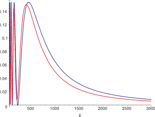
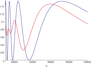
Figure 3: Probabilities $1-P_{\mu\mu}$ for the T2K experiment (left panel) and the CCFR experiment (right panel) for parameters indicated in table 1 and $U_{\mu 4}=0.2$. Red curves: the actual oscillation probabilities, blue curves: the oscillation probabilities in the case of neutrino emission from a single point located in the middle of the decay tunnel. Neutrino energies are in MeV.

9 Discussion

In the present paper we have studied in detail neutrino production coherence, which ensures that the emitted neutrino state is a coherent superposition of different mass eigenstates, as well as its implications for neutrino oscillations. We considered neutrino production using $\pi\to\mu\nu$ decay as an example. However, our analysis also applies to neutrinos produced in any other decay process (such as $K$-decay, $\mu$-decay, $\beta$-decay, etc.), provided that particles accompanying neutrino production are undetected, as it is usually the case.

We studied neutrino production coherence in two completely different approaches. In one of them, based on the quantum-mechanical wave packet formalism, we found the transition amplitude ${\cal A}_{\alpha\beta}(L,t)$ by summing the amplitudes of neutrino production at different points along the path of the parent particle. The oscillation probability $P_{\alpha\beta}(L)$ is then found by integrating the squared modulus of the obtained amplitude over time. In the second approach we assumed that each individual neutrino production event is fully coherent, so that the evolution of the produced neutrino should be described by the standard oscillation probability. However, the neutrino emission can occur (with some probability) at any point within the neutrino source, and therefore the effective oscillation probability is obtained by the proper averaging of the standard probability over the neutrino source. In both approaches we assumed that the neutrino detection process is perfectly localized.

We have found that in the case when the parent particles, in decays of which the neutrinos are produced, can be considered as pointlike, the results of the two approaches exactly coincide. This happens despite the fact that the first approach is fully quantum mechanical, while the second one, based on the probability summation, is essentially classical. We thus confirm the conclusion of ref. [3] where, along with the probability summation, a simplified treatment of the quantum mechanical coherent amplitude summation was given.

It should be stressed that the equivalence of the two approaches studied in this paper is different from the one discussed in [5, 25]. In those papers the authors have pointed out that it is impossible to distinguish experimentally between an ensemble of neutrinos described by wave packets, each with the energy distribution amplitude $g(E)$, and a beam of plane-wave neutrinos, each with well defined energy, but with the energy spectrum of the beam given by the squared modulus of the same function $g(E)$. In our case we establish the equivalence between a beam of neutrinos described by wave packets and a beam of pointlike neutrinos, which are just the opposites of the plane waves.

How can one understand the equivalence of the two approaches studied in this paper which takes place in the case of pointlike pions? Although the position of the pion decay (and neutrino production) point is not a priori exactly known, having uncertainty of order $l_{p}$ for $\Gamma l_{p}/v_{\pi}\ll 1$ and $l_{\rm decay}=v_{\pi}/\Gamma$ for $\Gamma l_{p}/v_{\pi}\gg 1$, the spatial size of the production region for each individual production event is very small: it is given by the size of the smallest wave packet of the particles participating in neutrino production, in our case of the pion. For pointlike pions the space-time localization of the detection process actually allows one, for each detection event, to pinpoint the coordinate of the neutrino emission. Thus, in this case there is no quantum mechanical uncertainty in the coordinate of neutrino production and therefore no interference between the amplitudes of neutrino emission from different (even closely located) points. This explains why our results obtained through the coherent summation of the amplitudes of neutrino production along the neutrino source coincide with those found by the simple incoherent summation of the oscillation probabilities.

From the above argument it follows that one can expect some deviations between the results of the coherent amplitude summation and incoherent probability summation approaches if pions are described by wave packets of finite size $\sigma_{x\pi}$. This is indeed confirmed by our treatment of the finite $\sigma_{x\pi}$ case in sections 4 and 6. We have found that for small $A_{\pi}\sim[v_{g}/(v_{g}-v_{\pi})](\Delta m^{2}/2P)\sigma_{x\pi}$ the oscillation probabilities get extra oscillatory terms proportional to $A_{\pi}$. For different shapes of the pion wave packets these corrections differ only by numerical factors (cf. eqs. (59) and  (65)). At the same time, for $A_{\pi}\gg 1$ the neutrino production coherence is violated, and the oscillatory terms in the oscillation probabilities are strongly suppressed. From the above discussion it should be rather obvious that the amplitude summation and probability summation approaches should lead to different results also in the case when the detection process is not perfectly localized, i.e. when the particles participating in neutrino detection are described by wave packets of finite size. This should be the case even if the production process is perfectly localized.

The above points as well as the role of detection of the charged lepton produced alongside the neutrino are illustrated by fig. 4. In this figure we present the space-time diagrams that correspond to six different experimental setups in the case of neutrinos produced in $\pi\to\mu\nu$ decays. The size of the region of coherent amplitude summation in each case is determined by the interplay of three factors, namely, whether the pion can be considered as pointlike or not and whether the neutrino and muon detection regions can be considered to be space-time points or not. Whenever this region degenerates to a point, the coherent and incoherent summation approaches yield identical results. For simplicity, in the cases when the neutrino and the muon detection processes are not fully localized, we display them as being extended in time but localized in space. More general situations where these processes are delocalized both in space and time can be readily studied; however, the corresponding results will not modify our qualitative conclusions. The six panels in fig. 4 thus illustrate the following situations:

• The pion and the neutrino detection region are both pointlike, the muon goes undetected. The first two conditions are sufficient to identify the point where the neutrino was produced, thus eliminating any quantum mechanical uncertainty in the emission coordinate. The oscillation probability found through the coherent amplitude summation must be identical to the one obtained by incoherent probability summation.

• The pion and the neutrino detection region are both pointlike, the muon detection region has a finite size. The latter does not restore coherence of neutrino emission from different points (illustrated by the dotted lines in the figure). The corresponding contributions have to be summed at the level of probabilities.

• The pion is of finite extension and so is the muon detection region, whereas the neutrino detection is pointlike. A one-dimensional region $AB$ is formed as the intersection of the regions corresponding to these three conditions. It is impossible in principle to determine from which point in the segment $AB$ the neutrino was emitted, and the amplitudes of neutrino emission from all such points thus interfere. The amplitude summation produces the results that are different from those found through the probability summation.

  Depending on the degree of its delocalization, the muon detection process may reduce the length of the segment $AB$ compared to the case when the muon is undetected (cf. figs. 2 and 4c) and thus diminish the effects of averaging of neutrino oscillations caused by neutrino production decoherence.

• The pion is of finite extension, the neutrino detection region is also finite, but the muon detection region is pointlike. As in c), the region of amplitude summation is a segment, and there is no equivalence with incoherent probability summation.

• Both pion and neutrino detection regions are of finite size, while the muon goes undetected. A 2-dimensional region of amplitude summation is formed; the amplitudes of neutrino emission from different points of this region interfere.

• Same as in e), but with muon detection (finite detection region). As in case e), the region of amplitude summation is 2-dimensional. Its size may be smaller than in case e) due to constraints from the muon detection.

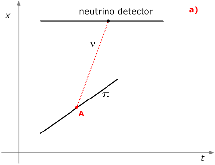
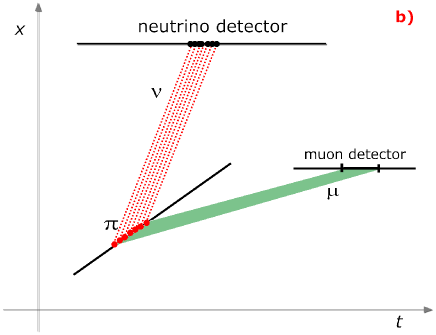
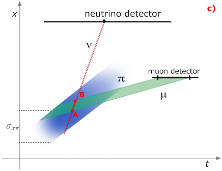
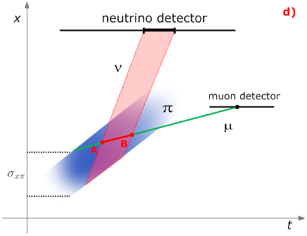
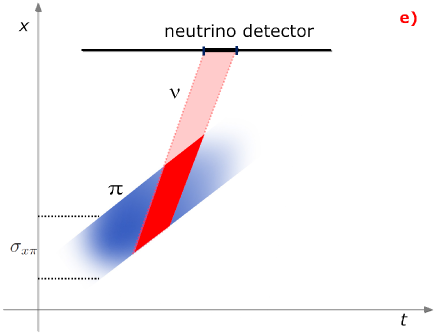
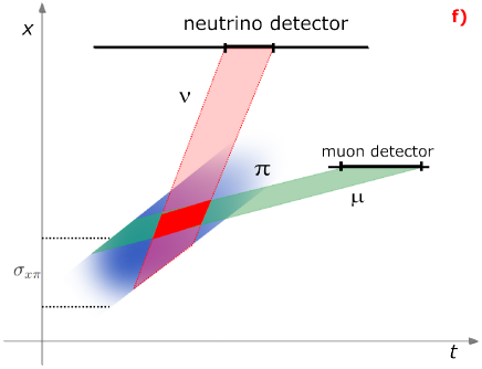
Figure 4: Space-time diagrams corresponding to six experimental setups. The regions of coherent production in each case are shown in deep red (see text).

Not shown in fig. 4 is one more case when the results of the amplitude summation and probability summation approaches coincide: neutrino detection region is of finite extension, whereas the pion is pointlike and the muon detection is perfectly localized in space an time.

Are deviations between the results of the coherent amplitude summation and incoherent probability summation approaches experimentally observable? Consider the case of perfectly localized neutrino detection, non-zero spatial widths of the pion wave packets and no muon detection (fig. 2). The corrections to the oscillation probabilities due to $\sigma_{x\pi}\neq 0$ are governed in this case by the parameter $A_{\pi}$ which, as follows from (59) or (65), can become sizeable for extremely high energies of the parent pion. This requires

$$2\left(E_{\pi}\sigma_{x\pi}\right)\frac{\Delta m^{2}}{m_{\pi}^{2}}\gtrsim 1\,.$$ (101)

For instance, if the width of the proton wave packets $\sigma_{xp}\sim 10^{-4}$ cm, one can expect also $\sigma_{x\pi}\lesssim 10^{-4}$ cm (see eq. (7)); for $\Delta m^{2}\sim 1$ eV² the parameter $A_{\pi}$ will then become of order one for pion energies $E_{\pi}\gtrsim 10^{3}$ TeV. Such energies are not feasible, and even if they were, the corresponding neutrino oscillation lengths would be far too large for any oscillation experiment. Another possibility to make $A_{\pi}$ sizeable would be to increase significantly the spatial width of the wave packets of ancestor protons, which would in turn increase the values of $\sigma_{x\pi}$. However, it is not clear how this can be achieved.

The two approaches to production decoherence effects that we followed in this paper describe the same physical phenomenon – the suppression of the oscillating terms in neutrino transition and survival probabilities due to delocalization of the production process. The nature of this suppression, however, is different in different situations.

In general, the proper description of the decoherence phenomenon requires using the quantum-mechanical approach with coherent summation of the amplitudes of neutrino production at different points. In this framework one considers the violation of production coherence due to lack of localization of each individual neutrino production event. This delocalization of neutrino production is related to the fact that the exact coordinate of the neutrino emission point is not known. The decoherence parameter is therefore essentially the ratio of the size of the neutrino production region and the neutrino oscillation length. As was shown in section 2, in the limit $\Gamma l_{p}/v_{\pi}\ll 1$ the decoherence parameter is $\phi_{p}=2\pi l_{p}/l_{\rm osc}$, whereas for $\Gamma l_{p}/v_{\pi}\gg 1$ it is $\xi=2\pi l_{\rm decay}/l_{\rm osc}$. The decoherence parameters can also be represented as the ratio of the energy difference of different neutrino mass eigenstates and the energy uncertainty inherent in the neutrino production (see section 2.5): $\Delta E/\sigma_{E}\approx\phi_{p}$ for $\Gamma l_{p}/v_{\pi}\ll 1$; $\Delta E/\sigma_{E}\approx\xi$ for $\Gamma l_{p}/v_{\pi}\gg 1$. For $\Delta E/\sigma_{E}\gtrsim 1$ the production process can discriminate between different neutrino eigenstates, leading to a loss of their coherence.

It is interesting to note that for decay of pointlike parent particles at rest ($v_{P}=0$) the production decoherence parameters vanish: the parameter $\xi$ vanishes because it is proportional to $v_{P}$, whereas $\phi_{p}$ is essentially zero because the effective size of the neutrino source $l_{p}$ is negligibly small for decay at rest. Physically, the reason for a perfect production coherence in the case $v_{\pi}\to 0$ (and good spatial localization of the neutrino detection process) is that the oscillation baseline is fixed and, in particular, is independent of the time when the parent pions decay. The oscillation baseline is not, however, fixed if the wave packets of the parent particles are of finite size; in this case the averaging of the oscillation phase over the widths of these wave packets can lead to decoherence effects.

In the second approach considered in the present paper it is assumed that the position of each neutrino emission point is exactly known. Each individual neutrino production event is assumed to be fully coherent, and the averaging of the production coordinate over the neutrino source is performed simply because the source is extended and the neutrino emission can occur in any place inside it. The averaging in this case is done at the probability level and is described by the parameter $\phi_{p}$ for $\Gamma l_{p}/v_{\pi}\ll 1$ and by $\xi$ for $\Gamma l_{p}/v_{\pi}\gg 1$. These parameters are just related to the effective size of the neutrino source, which in these limits is, respectively, $l_{p}$ and $l_{\rm decay}=v_{\pi}/\Gamma$. Actually, there is no notion of production decoherence in this case, and the suppression of the oscillatory terms in the probabilities is merely due to the averaging of the standard oscillation probability over the macroscopic sizes of the neutrino source and detector.

As we have discussed in detail, the two approaches turn out to be equivalent if the detection process is perfectly localized in space and time and in addition the spatial size of the wave packet of the parent particle can be neglected. This conclusion does not change if the particles accompanying the neutrino production (such as muon in $\pi\to\mu\nu$ decay) interact with the medium or are directly detected. However, if the detection of the accompanying particles is used for neutrino tagging, i.e. allows one to establish the coordinate of the neutrino emission point in the source with an accuracy $\sigma_{x\mu}$, this can affect the oscillation probabilities by reducing the averaging effects. In the case when the coherent amplitude summation does not reduce to the probability summation (e.g., for finite-size pion wave packets), this happens due to a better localization of individual neutrino production points (assuming that $\sigma_{x\mu}<l_{p}$, $l_{\rm decay}$), which improves the production coherence. In the case when the use of the probability summation is legitimate, neutrino tagging through the detection of the accompanying particles would just mean that the neutrinos are emitted not from the whole neutrino source, but from a region of it of the effective size $\sigma_{x\mu}$. The integration over the coordinate of the neutrino production should then be carried out only over this region.

In conclusion, we have identified the condition under which coherent and incoherent summations over points in the neutrino production region yield different oscillation results. This condition can be succinctly stated as follows: the two approaches lead to different results whenever the localization properties of the parent particles at neutrino production and of the detection process are such that they prevent the precise localization of the point of neutrino emission. The difference in the oscillation results is negligible for present accelerator experiments, and therefore the standard averaging of the oscillation probabilities over the finite spatial extensions of the neutrino source and detector properly takes decoherence effects into account. Whether it is possible to devise a realistic experiment that could probe this difference remains to be seen.

The authors are grateful to Thomas Schwetz and Manfred Lindner for useful discussions.

References

- [1] B. Kayser, Phys. Rev. D 24 (1981) 110.
- [2] See the talks at Sterile Neutrinos at Crossroads, Blacksburg, USA, September 25-28, 2011, http://www.cpe.vt.edu/snac/program.html.
- [3] D. Hernandez, A. Yu. Smirnov, arXiv:1105.5946 [hep-ph].
- [4] E. Kh. Akhmedov, A. Yu. Smirnov, Phys. Atom. Nucl. 72 (2009) 1363-1381 (shortened version). The full version is in arXiv:0905.1903 [hep-ph].
- [5] J. Rich, Phys. Rev. D 48 (1993) 4318.
- [6] C. Giunti, JHEP 0211 (2002) 017 [hep-ph/0205014].
- [7] M. Beuthe, Phys. Rept. 375 (2003) 105 [arXiv:hep-ph/0109119].
- [8] E. Kh. Akhmedov, J. Kopp, JHEP 1004 (2010) 008 [arXiv:1001.4815 [hep-ph]].
- [9] D. Bohm, Quantum theory, Dover, 1989.
- [10] C. Giunti, C. W. Kim and U. W. Lee, Phys. Rev. D 44 (1991) 3635.
- [11] C. Giunti and C. W. Kim, Phys. Rev. D 58 (1998) 017301 [arXiv:hep-ph/9711363].
- [12] Y. Farzan, A. Y. Smirnov, Nucl. Phys. B805 (2008) 356-376. [arXiv:0803.0495 [hep-ph]].
- [13] A. Aguilar et al. [LSND Collaboration], Phys. Rev. D 64 (2001) 112007 [hep-ex/0104049].
- [14] B. Armbruster et al. [KARMEN Collaboration], Phys. Rev. D 65 (2002) 112001 [hep-ex/0203021].
- [15] E. D. Zimmerman [for the MiniBooNE Collaboration], arXiv:1111.1375 [hep-ex].
- [16] P. Astier et al. [NOMAD Collaboration], Nucl. Phys. B 611 (2001) 3 [hep-ex/0106102].
- [17] D. Naples et al. [CCFR/NuTeV Collaboration], Phys. Rev. D 59 (1999) 031101 [hep-ex/9809023].
- [18] F. Dydak, G. J. Feldman, C. Guyot, J. P. Merlo, H. J. Meyer, J. Rothberg, J. Steinberger and H. Taureg et al., Phys. Lett. B 134 (1984) 281.
- [19] M. H. Ahn et al. [K2K Collaboration], Phys. Rev. D 74 (2006) 072003 [hep-ex/0606032].
- [20] F. Di Lodovico for the T2K Collaboration, arXiv:1110.5382 [hep-ex]; K. Abe et al. [T2K Collaboration], Nucl. Instrum. Meth. A 659 (2011) 106 [arXiv:1106.1238].
- [21] P. Adamson et al. [MINOS Collaboration], Phys. Rev. Lett. 107 (2011) 011802 [arXiv:1104.3922 [hep-ex]].
- [22] G. S. Davies for the Nova Collaboration, arXiv:1110.0112 [hep-ex].
- [23] P. Zucchelli, Phys. Lett. B 532 (2002) 166.
- [24] S. K. Agarwalla, P. Huber and J. M. Link, JHEP 1001 (2010) 071 [arXiv:0907.3145 [hep-ph]].
- [25] K. Kiers, S. Nussinov and N. Weiss, Phys. Rev. D 53 (1996) 537 [hep-ph/9506271].