Local anisotropy, higher order statistics, and turbulence spectra

Abstract

Correlation anisotropy emerges dynamically in magnetohydrodynamics (MHD), producing stronger gradients across the large-scale mean magnetic field than along it. This occurs both globally and locally, and has significant implications in space and astrophysical plasmas, including particle scattering and transport, and theories of turbulence. Properties of local correlation anisotropy are further documented here by showing through numerical experiments that the effect is intensified in more localized estimates of the mean field. The mathematical formulation of this property shows that local anisotropy mixes second-order with higher order correlations. Sensitivity of local statistical estimates to higher order correlations can be understood in connection with the stochastic coordinate system inherent in such formulations. We demonstrate this in specific cases, illustrate the connection to higher order statistics by showing the sensitivity of local anisotropy to phase randomization, and thus establish that the local structure function is not a measure of the energy spectrum. Evidently the local enhancement of correlation anisotropy is of substantial fundamental interest, and this phenomenon must be understood in terms of higher order correlations, fourth-order and above.

1. Introduction: correlations and anisotropy

Correlation and spectral anisotropy play important roles in current studies of solar wind and astrophysical plasmas, having significant impact on descriptions of the turbulence cascade, particle scattering, the nature of kinetic dissipation, and the transport of turbulence. Evidence from experiments, numerical simulations, theoretical arguments, and spacecraft observations has consistently supported the conclusion that magnetohydrodynamic (MHD) turbulence leads to states characterized by gradients that are relatively stronger when measured perpendicular to the large-scale magnetic field and relatively weaker when measured parallel to it (Robinson & Rusbridge, 1971; Zweben et al., 1979; Ren et al., 2011; Shebalin et al., 1983; Bondeson, 1985; Carbone & Veltri, 1990; Oughton et al., 1994; Montgomery & Turner, 1981; Matthaeus et al., 1990; Bieber et al., 1996). This correlation anisotropy has been quantified both globally and locally, by varying the definition of the mean magnetic field. The local form, being of greater magnitude, has received substantial attention in recent years (Cho & Vishniac, 2000; Milano et al., 2001; Horbury et al., 2008; Tessein et al., 2009; Podesta, 2009; Luo & Wu, 2010; Wicks et al., 2010, 2011; Chen et al., 2011). The present paper will focus on the relationship between these forms of anisotropy, providing a better characterization of the scale dependence of local anisotropy. A particular conclusion will be that correlation anisotropy affects statistics at all orders, including but not limited to the energy spectrum and other second-order statistics. We also present evidence that the enhancement of local anisotropy over the global value is due entirely to higher order statistical effects.

The basic physics leading to this strong perpendicular spectral transfer and enhancement of perpendicular anisotropy has been elucidated in the context of incompressible homogeneous MHD turbulence (Montgomery & Turner, 1981; Shebalin et al., 1983; Bondeson, 1985; Grappin, 1986; Oughton et al., 1994). For this model, all modal couplings are triadic (involving wavevectors $\boldsymbol{k}_{1}$, $\boldsymbol{k}_{2}$, $\boldsymbol{k}_{3}$, such that $\boldsymbol{k}_{1}+\boldsymbol{k}_{2}+\boldsymbol{k}_{3}=0$), but in the presence of a strong uniform DC magnetic field $B_{0}\hat{\boldsymbol{z}}$, only those couplings that have one (or all three) wavevectors perpendicular to $\hat{\boldsymbol{z}}$ will proceed unattenuated by propagation effects. All other couplings are suppressed to a progressively greater degree as $B_{0}$ is strengthened. The appearance of stronger perpendicular gradients implies that spectral transfer to the perpendicular wavevectors is more robust than that to the parallel wavenumbers. This corresponds to appearance of characteristic spectral anisotropy, with enhancements of high $k_{\perp}$ power relative to $k_{\parallel}$ power, an effect that become progressively stronger at smaller scales (Shebalin et al., 1983; Oughton et al., 1994). This organization of the spectrum, is built into models such as Reduced MHD (RMHD) (Kadomtsev & Pogutse, 1974; Strauss, 1976; Montgomery, 1982) and related models such as the Goldreich & Sridhar (1995) steady-state (GS) model, and the nearly incompressible MHD (NIMHD) model (Zank & Matthaeus, 1992). Indeed strong anisotropy of MHD correlations is observed in laboratory devices (Robinson & Rusbridge, 1971; Zweben et al., 1979; Ren et al., 2011), in the solar wind (Matthaeus et al., 1990; Tu & Marsch, 1995; Bieber et al., 1996) and the corona (Armstrong et al., 1990), and is an apparent requirement for consistency of scattering theory with solar energetic particle (SEP) observations (Bieber et al., 1994; Dröge, 2005).

However anisotropy of the energy spectrum is not the only effect associated with correlation anisotropy and enhancement of perpendicular gradients. For example, one can discuss the shape and orientation of structures, such as “eddies” (Cho & Vishniac, 2000) or current sheets (Dmitruk et al., 2004). It is well known that one of the powerful nonlinear effects of turbulence is the production of coherent structures that are progressively smaller at small scales. This leads to intermittency as measured by nonGaussianity and higher order statistics, as seen in hydrodynamic and MHD models (She & Lévêque, 1994; Politano & Pouquet, 1995). Simulations show that such nonGaussian statistics are generated very rapidly by the cascade of excitations to smaller scales (Wan et al., 2009). In MHD, under a wide variety of conditions, the associated coherent structures take the form of enhancements of electric current density in sheets or filaments (Matthaeus & Lamkin, 1986; Carbone et al., 1990; Veltri, 1999). When the turbulence is anisotropic relative to a large-scale field (e.g., Dmitruk et al., 2004), the current structures tend to align in that direction as well. This suggests that higher order statistical quantities (fourth-order moments, kurtosis, etc) also must become anisotropic.

The above reasoning leads to an expectation that statistics at all orders might be involved in correlation anisotropy, but many “theories of MHD turbulence” discuss exclusively the properties of the second-order statistics; that is, the energy spectra and associated correlation and structure functions. This emphasis follows naturally from the use of wavevector spectra and two-point, single time correlation functions as measures of the distribution of energy in spatial structures of varying size (Monin & Yaglom, 1971, 1975), as exemplified by the classic Kolmogorov (1941) theory. Recognizing this background, it is not entirely surprising that recent interest in local anisotropy has sometimes focused on an interpretation of this effect as a local energy spectrum (Cho & Vishniac, 2000; Chen et al., 2011; Wicks et al., 2011). The discussion below provides in effect a critique of this interpretation.

To render the discussion specific, we assume a statistical description that is homogeneous in space and stationary in time. The brackets $\langle\cdots\rangle$ denote an ensemble average, which by invoking a classical ergodic theorem is approximated in practice by a space or time average. It may be possible to define the statistical ensemble in other ways, but here a classical statistical framework is assumed (Monin & Yaglom, 1971, 1975). The two-point correlation function measuring the statistical relationship between the magnetic field fluctuation at points $\boldsymbol{x}$ and displaced position $\boldsymbol{x}^{\prime}=\boldsymbol{x}+\boldsymbol{r}$ is also the Fourier transform of the wavevector energy spectrum, $S_{\alpha\beta}(\boldsymbol{k})$. The definitions are (e.g., Monin & Yaglom, 1971, 1975)

$$R_{\alpha\beta}(\boldsymbol{r})=\langle b_{\alpha}b^{\prime}_{\beta}\rangle=\int\mathrm{d}^{3}k\,\ S_{\alpha\beta}(\boldsymbol{k})e^{i\boldsymbol{k}\cdot\boldsymbol{r}},$$ (1)

where we abbreviate $b_{\alpha}=b_{\alpha}(\boldsymbol{x},t)$ and $b^{\prime}_{\beta}=b_{\beta}(\boldsymbol{x}+\boldsymbol{r},t)$, and suppress the time argument. Another two-point statistic is the second-order structure function

$$D(\boldsymbol{r})=\langle|\boldsymbol{b}-\boldsymbol{b}^{\prime}|^{2}\rangle\equiv 2\delta b^{2}-2R(\boldsymbol{r}),$$ (2)

which is obviously related to $R_{\alpha\beta}$. Here $\delta b^{2}=R_{\alpha\alpha}(0)$ is the total variance of the fluctuations and $R(\boldsymbol{r})=R_{\alpha\alpha}(\boldsymbol{r})$.

Existence of a homogeneous statistical ensemble implies that there exists a probability density ${\cal P}(\Gamma)$ that describes fully all realizations of the turbulence, where each realization is labeled by an index $\Gamma$. This density may be projected onto the space of two-point statistics, arriving at a probability distribution function (pdf) $P_{2}(\boldsymbol{b},\boldsymbol{b}^{\prime})$ that characterizes all of the two-point statistics of any order. Thus one may equivalently express the structure function in two ways as

$$D(\boldsymbol{r}) = \int_{\Gamma}\mathrm{d}\Gamma\,\left[|\boldsymbol{b}-\boldsymbol{b}^{\prime}|^{2}\right]_{\Gamma}{\cal P}(\Gamma)$$ (3)

$$= \iint\mathrm{d}^{3}b\,\mathrm{d}^{3}b^{\prime}\,\left|\boldsymbol{b}-\boldsymbol{b}^{\prime}\right|^{2}P_{2}(\boldsymbol{b},\boldsymbol{b}^{\prime}),$$ (4)

where $\left[|\boldsymbol{b}-\boldsymbol{b}^{\prime}|^{2}\right]_{\Gamma}$ is the value of the square-bracketed quantity for realization $\Gamma$. Similar relations hold for the spectra and two-point correlation functions. Note that the structure function $D$ and the correlation matrix $R_{\alpha\beta}$ are “second-order statistics” because they are explicitly written as second-order moments of either the full density $\cal P$ or of the reduced two-point probability density $P_{2}$.

In general the turbulence may not be isotropic, especially if $\langle\boldsymbol{B}\rangle=\boldsymbol{B}_{0}\neq\boldsymbol{0}$. It is then of interest to compute correlations in directions relative to $\hat{\boldsymbol{B}}_{0}=\boldsymbol{B}_{0}/B_{0}$ (and a perpendicular direction $\hat{\boldsymbol{n}}_{0}$). We will also consider a locally defined mean field in which the local mean direction $\hat{\boldsymbol{H}}=\boldsymbol{H}/|\boldsymbol{H}|$ is itself a random variable that satisfies $\langle\boldsymbol{H}\rangle=\boldsymbol{B}_{0}$. We have in mind several possible ways to determine $\boldsymbol{H}$, for example as $\boldsymbol{H}_{V}(\boldsymbol{x})=V^{-1}\int_{V}\mathrm{d}^{3}r\,\boldsymbol{B}$, defined in subvolumes or “boxes” of volume $V$ centered on $\boldsymbol{x}$; or as $\boldsymbol{H}_{L}=L^{-1}\int_{L}\mathrm{d}r\,\boldsymbol{B}$, defined in co-linear samples of length $L$ (as used in single spacecraft estimates in the solar wind, under Taylor’s hypothesis); or perhaps as $\boldsymbol{H}_{\boldsymbol{r}}(\boldsymbol{x})$ defined as the average of $\boldsymbol{B}$ at ${\boldsymbol{x}}$ and $\boldsymbol{x}^{\prime}$, $\frac{1}{2}\left[\boldsymbol{B}(\boldsymbol{x}+\boldsymbol{r})+\boldsymbol{B}(\boldsymbol{x})\right]$. These may be called, respectively, volume averages, line averages, and point averages.

At this point we recall a generalization of standard structure functions (Milano et al., 2001) that formally coincides with $D(\boldsymbol{r})$,

$$\tilde{D}(s)\equiv\langle|\boldsymbol{b}(\boldsymbol{x})-\boldsymbol{b}(\boldsymbol{x}+s\hat{\boldsymbol{c}})|^{2}\rangle,$$ (5)

except that the direction $\hat{\boldsymbol{c}}$ is permitted to be a variable direction, in particular a direction determined relative to the local estimates $\hat{\boldsymbol{H}}$. For special cases, the separation can be chosen to be either parallel to the local mean magnetic field, $\hat{\boldsymbol{c}}\to\hat{\boldsymbol{H}}$, or else perpendicular to $\boldsymbol{H}$: $\hat{\boldsymbol{c}}\to\hat{\boldsymbol{n}}\equiv\hat{\boldsymbol{e}}\times\hat{\boldsymbol{H}}/|\hat{\boldsymbol{e}}\times\hat{\boldsymbol{H}}|$ for reference direction $\hat{\boldsymbol{e}}$. This enables us to define the (locally) parallel structure function $\tilde{D}^{\parallel}(s)=\langle|\boldsymbol{b}(\boldsymbol{x})-\boldsymbol{b}(\boldsymbol{x}+s\hat{\boldsymbol{H}})|^{2}\rangle$ and the local perpendicular (transverse) structure function $\tilde{D}^{\perp}(s)=\langle|\boldsymbol{b}(\boldsymbol{x})-\boldsymbol{b}(\boldsymbol{x}+s\hat{\boldsymbol{n}})|^{2}\rangle$. Our main concern here will be to better understand the relationship between local and global anisotropy, and between $D$ and $\tilde{D}$. We conclude that however appealing their similarity might be, one can anticipate fundamental differences. Notably, since $\tilde{D}$ is defined in a stochastic coordinate system it is thus a conditional statistic. $\tilde{D}$ is therefore necessarily a higher order statistical quantity. In contrast, $D$ is defined in a fixed coordinate system and is related directly to the second-order statistics, such as correlation functions and spectra.

Milano et al. (2001) showed that structure functions defined as above can be employed to quantify both global anisotropy and local anisotropy. For separations $s$ lying in the inertial range and smaller, and for cases with nonzero $B_{0}$, global anisotropy takes the form $D(s\hat{\boldsymbol{n}}_{0})/D(s\hat{\boldsymbol{B}}_{0})>1$, which is equivalent to enhanced perpendicular anisotropy seen in spectra (Shebalin et al., 1983; Oughton et al., 1994). Local anisotropy is typically characterized by $\tilde{D}^{\perp}(s)/\tilde{D}^{\parallel}(s)>1$, which corresponds to stronger gradients perpendicular to a local preferred direction. Interestingly, the local anisotropy was found to be greater than the global anisotropy at a given scale, $\tilde{D}^{\perp}(s)/\tilde{D}^{\parallel}(s)>D(s\hat{\boldsymbol{n}}_{0})/D(s\hat{\boldsymbol{B}}_{0})>1$ (Milano et al., 2001). It is noteworthy that local anisotropy was found even in cases that are globally isotropic with $B_{0}=0$. A related study (Cho & Vishniac, 2000) found similar local anisotropy, and argued for a correspondence to anisotropic magnetic spectra in the “reduced MHD” regime (Goldreich & Sridhar, 1995).

2. Results

Milano et al. (2001) also suggested that there was evidence for progressively greater anisotropy as the mean field is computed more locally. However the available bandwidth of the simulations limited the strength of that conclusion. We present a new result here that demonstrates this effect with higher resolution simulations, employing (dealiased) incompressible 3D MHD spectral method simulations at a spatial resolution of $512^{3}$. Thus the maximum retained wavenumber is $k_{\text{max}}=170$ ($k=1$ corresponds to the longest allowed wavelength in the periodic box). The runs are initial value problems, decaying turbulence with initially excited wavenumbers of $k=1$ to $6$, and initial fluctuation energy normalized such that $\langle\boldsymbol{b}\cdot\boldsymbol{b}\rangle=\langle\boldsymbol{v}\cdot\boldsymbol{v}\rangle=1$. The resistivity $\mu$ and viscosity $\nu$, are selected to ensure good spatial resolution, meaning that $k_{\text{max}}/k_{\text{diss}}>3$ at all times (Wan et al., 2010). The dissipation wavenumber is defined as $k_{\text{diss}}=1/\lambda_{\text{diss}}=(\epsilon/\nu^{3})^{1/4}$, where $\epsilon$ is the rate of (total) energy dissipation. Initial Reynolds numbers are $R=1/\nu=Rm=1/\mu=2000$.

We report on two runs, one with $B_{0}=0$ and another with $B_{0}=1$. Broadband energy spectra develop and the data are analyzed near the time of maximum dissipation. We examined the anisotropy relative to local mean fields determined variously as volume, line and point averages. Corresponding estimates of $\tilde{D}^{\parallel}(s)$ and $\tilde{D}^{\perp}(s)$ were computed in the same way. For volume averages, or line averages with $V^{1/3}\sim L\gg\lambda_{c}$, the correlation scale of the fluctuations, we expect that $\boldsymbol{H}_{V}$ provides increasingly refined estimates of $\boldsymbol{B}_{0}$. Indeed, for one dimensional random process, the classical ergodic theorem (Monin & Yaglom, 1971, 1975) guarantees that ${\lim}_{L\to\infty}\boldsymbol{H}_{L}=\langle\boldsymbol{B}\rangle=\boldsymbol{B}_{0}$.

To assess the degree of local anisotropy, the local structure functions are computed a locally-determined mean-field-aligned axisymmetric coordinate system. That is, estimates of $\tilde{D}^{\parallel}(s)$ and $\tilde{D}^{\perp}(s)$ are accumulated and averaged. Several methods are used to determine the local mean field – volume, line and point averaging, as described above. Figure 1 shows the ratio $\tilde{D}^{\perp}(s)/\tilde{D}^{\parallel}(s)$ which provides a measure of the variation of anisotropy with lag $s$, for several different determinations of the local mean field. Also shown is the anisotropy ratio relative to the global mean magnetic field. It is clear that (1) the degree of anisotropy is greater at smaller lags; and (2) that anisotropy is more pronounced when the mean magnetic field is computed over a smaller region. This was found by Milano et al. (2001) and Cho & Vishniac (2000) and confirmed in numerous other studies. As has been reported previously, local anisotropy is present not only for the nonzero $B_{0}$ case (Fig. 1b) but also for zero global mean field (Fig 1a). We thus confirm that stronger gradients are produced perpendicular to the magnetic field, and also that local anisotropy is stronger than global anisotropy.

Clearly the local structure functions are of great interest, and we now discuss their formal nature. It is convenient to introduce the generalization $\tilde{D}(s_{\parallel},s_{\perp})=\langle|\boldsymbol{b}(\boldsymbol{x})-\boldsymbol{b}(\boldsymbol{x}+s_{\parallel}\hat{\boldsymbol{H}}+s_{\perp}\hat{\boldsymbol{n}})|^{2}\rangle$, which makes explicit the possibility of arbitrary separations, both parallel ($s_{\parallel}$) to and perpendicular ($s_{\perp}$) to the local mean magnetic field. Evidently $\tilde{D}^{\parallel}(s)=\tilde{D}(s,0)$ and $\tilde{D}^{\perp}(s)=\tilde{D}(0,s)$.

The quantity $\tilde{D}$ can be formally obtained from the expression for $D(\boldsymbol{r})$ in Eq. (2) by the replacement $\boldsymbol{r}\to s_{\parallel}\hat{\boldsymbol{H}}+s_{\perp}\hat{\boldsymbol{n}}$ in Eq. (4). However some care is required in interpreting this procedure due to the new stochastic variables that appear in the arguments. (For example, the implication is that the differential $\mathrm{d}^{3}b^{\prime}$ becomes stochastic.) To avoid complications we choose to write the defining relation in terms of the full probability density of realizations, that is,

$$\tilde{D}(s_{\parallel},s_{\perp})=\int_{\Gamma}\mathrm{d}\Gamma\left[|\boldsymbol{b}(\boldsymbol{x}+s_{\parallel}\hat{\boldsymbol{H}}+s_{\perp}\hat{\boldsymbol{n}})-\boldsymbol{b}(\boldsymbol{x})|^{2}\right]_{\Gamma}{\cal P}(\Gamma).$$ (6)

This new expression is not a simple coordinate transformation of Eq. (4) because the coordinate unit vectors $\hat{\boldsymbol{H}}$ and $\hat{\boldsymbol{n}}$ are themselves random variables, dependent upon $\Gamma$. However the new independent variables $s_{\parallel}$ and $s_{\perp}$ are non-random coordinates in the stochastically rotated reference frame of the local systems. It is clear that $\tilde{D}(s_{\parallel},s_{\perp})$ remains a second-order statistical quantity only if the coordinate system is fixed and $\hat{\boldsymbol{H}}$ and $\hat{\boldsymbol{n}}$ become fixed vectors, or if the probability distributions are insensitive to directions. The former case is obtained asymptotically as $B_{0}\to\infty$ and the mean field direction becomes statistically sharp. The latter case is obtained for highly symmetric cases such as isotropic turbulence. In general, unless the density $\cal P$ is invariant under the stochastic changes of $\boldsymbol{H}$, the statistical nature of $\tilde{D}$ becomes higher order.

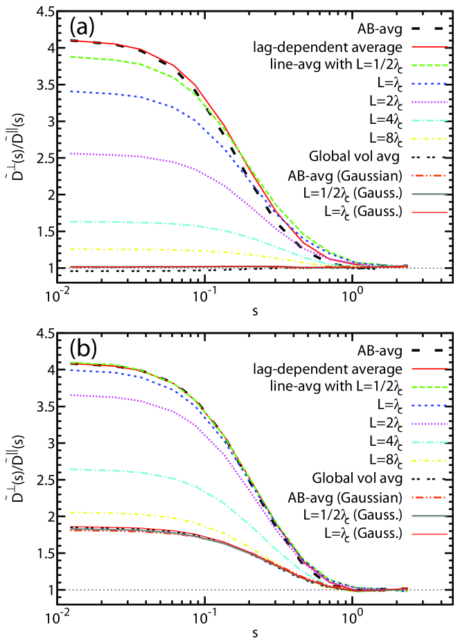
Figure 1.— Anisotropy ratio $\tilde{D}^{\perp}(s)/D^{\parallel}(s)$ vs. lag $s$ at inertial range and larger scales. Point and line average estimates of local mean field $\boldsymbol{H}$ are used (“AB” averages the two points $\boldsymbol{x}$, $\boldsymbol{x}^{\prime}$, “lag dependent” integrates from $\boldsymbol{x}$ to $\boldsymbol{x}^{\prime}$.) Perpendicular excitation is relatively enhanced, except for lags $s\gtrsim 1$ where isotropy holds (N.B. energy containing eddies are initially isotropic). (a) Results from $B_{0}=0$ simulation, with $\lambda_{c}=0.34$ and $\lambda_{\text{diss}}=0.021$. Anisotropy is stronger for more localized estimates of $\boldsymbol{H}$ (e.g., shorter line averages). Randomizing phases (Gaussianizing – see text), produces isotropic results for all averaging methods and at all lags. Therefore, anisotropy is associated with non-Gaussian correlations. (b) Results from $B_{0}=1$ simulation, with $\lambda_{c}^{\perp}=0.34$, $\lambda_{c}^{\parallel}=0.43$, and $\lambda_{\text{diss}}=0.022$. This case is anisotropic relative to the globally determined $\boldsymbol{B}_{0}$, and all methods based on local determinations of the mean field show further enhancement of anisotropy. For this run, phase randomization removes the enhanced local anisotropy, but global anisotropy remains.

The latter point and its consequences can be made more explicit by considering special cases. For small separations purely in the parallel direction ($s_{\perp}=0$ and small $s_{\parallel}$), and considering the decomposition $\boldsymbol{H}\equiv\boldsymbol{B}_{0}+\boldsymbol{h}$, we may expand

$$\tilde{D}(s,0) = \langle|s\hat{\boldsymbol{H}}\cdot\nabla\boldsymbol{b}(\boldsymbol{x})+\frac{s^{2}}{2}\hat{\boldsymbol{H}}_{i}\hat{\boldsymbol{H}}_{j}\nabla_{i}\nabla_{j}\boldsymbol{b}(\boldsymbol{x})+{\cal O}(s^{3})|^{2}\rangle$$ (7)

$$= s^{2}\langle{|\widehat{(\boldsymbol{B}_{0}+\boldsymbol{h})}\cdot\nabla\boldsymbol{b}|^{2}}\rangle+{\cal O}(s^{3}).$$

Suppose that $|\boldsymbol{b}|/B_{0}\ll 1$ is small enough to justify an additional expansion in that parameter. This yields $\tilde{D}(s,0)=s^{2}\hat{\boldsymbol{B}}_{0i}\hat{\boldsymbol{B}}_{0j}\langle(\nabla_{i}b_{k})(\nabla_{j}b_{k})\rangle+{\cal O}(hbb/B_{0})$. The first term is a second-order moment. The remaining terms include third, fourth, and higher-order moments. Only in the asymptotic limit, in which $\boldsymbol{H}\to\boldsymbol{B}_{0}$, is a second-order moment recovered.

As a second special case suppose that (i) $B_{0}=0$, so the global anisotropy may be zero, and (ii) that the local mean field estimate is completely localized so that $\boldsymbol{H}=\boldsymbol{h}=\boldsymbol{b}$. Then once again beginning with the small $s$ expansion Eq. (7), we find that $\tilde{D}(s,0)=s^{2}\langle|\boldsymbol{b}\cdot\nabla\boldsymbol{b}|^{2}/|\boldsymbol{b}|^{2}\rangle+{\cal O}(s^{3})$, which involves moments higher than second-order. Even in the very special case that the magnetic field fluctuation is “arc polarized” and has constant magnitude $\sigma$, this still only reduces to a fourth-order quantity $\tilde{D}(s,0)\approx(s^{2}/\sigma^{2})\langle|\boldsymbol{b}\cdot\nabla\boldsymbol{b}|^{2}\rangle$.

Observing that the relationship between the structure function $D(\boldsymbol{r})$ and the local field aligned structure function $\tilde{D}$ is somewhat analogous in form to the relationship between Eulerian and Lagrangian correlation functions, one might be tempted to seek similar approximations to connect them. One possibility, based on the ideas underlying Corrsin’s hypothesis of independence (see, e.g., McComb (1990)) is to treat the distribution of the magnetic field fluctuations as independent of the distribution of the mean magnetic field directions. Thus, symbolically one might attempt an approximation such as $P_{3}(\boldsymbol{b},\boldsymbol{b}^{\prime},\hat{\boldsymbol{H}})\to P_{2}(\boldsymbol{b},\boldsymbol{b}^{\prime})P_{H}(\hat{\boldsymbol{H}})$, from which it would follow that $\tilde{D}(s_{\parallel},s_{\perp})=\int\mathrm{d}\Omega_{H}\,C(s_{\parallel}\hat{\boldsymbol{H}}+s_{\perp}\hat{\boldsymbol{n}})P_{H}(\hat{\boldsymbol{H}})$, where $P_{H}(\hat{\boldsymbol{H}})$ is the distribution of mean field directions and $\mathrm{d}\Omega_{H}$ the differential of solid angles associated with those directions. However such an approximation must fail, as can be readily seen: Suppose that $C(\boldsymbol{r})$ has a strong perpendicular anisotropy. Then the random distribution of mean field directions $P_{H}$ will dull the sharpness of the anisotropy by averaging parallel separations with perpendicular separations. This independence hypothesis would thus produce local anisotropy that is weaker than the global anisotropy. This is inconsistent with both simulation results and solar wind results and therefore this approximation is invalid for the turbulence of interest.

In order to demonstrate their dependence on higher order correlations, we examined numerically the effect on local anisotropy of a Gaussianization or phase-randomization process. This procedure was carried out for the same simulation dataset described above. In particular for both the $B_{0}=0$ and $B_{0}=1$ cases, we modified the Fourier coefficients by randomizing their phases while keeping their magnitudes unchanged. The effect of phase randomization is to produce a signal that is Gaussian, lacking coherency associated with phase correlations. However this process does not modify the energy spectrum. Employing the phase randomized signal, we again compute the locally defined structure functions using the same set of methods for determining the local mean field that was described earlier. The scaling of the anisotropy with lag is shown in Fig. 1, where it is compared with the original simulation data for which phase coherency, if present, was maintained. The phase randomization has a dramatic effect in both cases: when there is global isotropy, the phase randomization completely destroys the local anisotropy. When there is global anisotropy the phase randomization completely eliminates the local enhancement of anisotropy.

3. Discussion

The issues described above appear to have immediate relevance to a number of analysis procedures that rely on local accumulation of data. For example, even apart from the issue of anisotropy, the discussions presented here are also relevant to studies that for various reasons employ short datasets to define a “mean” magnetic field and similarly local correlation or structure functions. Invariably use of short intervals (less than $\lambda_{c}$, or its temporal equivalent) time series leads to poorly determined global statistics, although an interpretation in terms of local conditional statistics may still be meaningful (e.g., Sahraoui et al., 2009, 2010; Alexandrova et al., 2011). However, the connection to various orders of statistics needs to be established.

Another popular approach is to employ wavelet techniques to determine “local spectra” as well as measures of local anisotropy analogous to $\tilde{D}$ (e.g., Horbury et al., 2008; Wicks et al., 2010, 2011; Chen et al., 2011). This approach is also based on conditional statistics, since it determines a local mean field at each scale and then accumulates data relative to the direction of that local mean field. It follows that such wavelet spectra will also be higher (than second) order statistical quantities, and thus are distinct from the actual spectra.

In conclusion, an examination of structure functions computed relative to locally determined mean magnetic field directions reveals that such quantities involve higher than second-order moments of the underlying probability distributions. This property emerges because the local mean field direction becomes a random variable. Consequently these structure functions are computed in a stochastic coordinate system, and involve averaging over the magnetic field at two positions, $\boldsymbol{b}$, and $\boldsymbol{b}^{\prime}$, and also the mean magnetic field direction $\hat{\boldsymbol{H}}$. Observing that the energy spectrum and related structure function are second-order moments, the fact that the locally-oriented structure functions involve higher order moments implies that the information they contain is not identical to that of the energy spectrum. The additional random degree of freedom does not appear to be amenable to an adaptation of the Corrsin independence hypothesis, given that the local anisotropy is stronger than the global anisotropy. Gaussianization (phase randomization) of a turbulent field eliminates the enhancement of the local anisotropy, confirming its sensitivity not just to higher order correlations, but in particular to higher order nonGaussian correlations. Evidently the phenomenon of locally enhanced anisotropy involves fundamental physics that is embedded in the higher order statistics, as is the case for intermittency and coherent structures that are generated by turbulence. This information is beyond the scope of what can properly be described with just the energy spectrum.

We thank Randy Jokipii for useful discussions. This research is partially supported by NASA (Heliophysics Theory) NNX11AJ44G, (Heliophysics GI) NNX09AG31G and NSF- (Solar Terrestrial) AGS-1063439 & (SHINE) ATM-0752135, and by the EU under the Marie Curie “TURBOPLASMA” project.

References

- Alexandrova et al. (2011) Alexandrova, O., Lacombe, C., Mangeney, A., & Grappin, R. 2011, ArXiv e-prints
- Armstrong et al. (1990) Armstrong, J., Coles, W., Kojima, M., & Rickett, B. 1990, Astrophys. J., 358, 685
- Belcher & Davis (1971) Belcher, J. W., & Davis, L., Jr. 1971, J. Geophys. Res., 76, 3534
- Bieber et al. (1994) Bieber, J. W., Matthaeus, W. H., Smith, C. W., Wanner, W., Kallenrode, M., & Wibberenz, G. 1994, Astrophys. J., 420, 294
- Bieber et al. (1996) Bieber, J. W., Wanner, W., & Matthaeus, W. H. 1996, J. Geophys. Res., 101, 2511
- Bondeson (1985) Bondeson, A. 1985, Phys. Fluids, 28, 2406
- Carbone & Veltri (1990) Carbone, V., & Veltri, P. 1990, Geophys. Astrophys. Fluid Dyn., 52, 153
- Carbone et al. (1990) Carbone, V., Veltri, P., & Mangeney, A. 1990, Phys. Fluids, 2, 1487
- Chen et al. (2011) Chen, C. H. K., Mallet, A., Yousef, T. A., Schekochihin, A. A., & Horbury, T. S. 2011, Mon. Not. R. Astron. Soc., 843
- Cho & Vishniac (2000) Cho, J., & Vishniac, E. T. 2000, Astrophys. J., 539, 273
- Dmitruk et al. (2004) Dmitruk, P., Matthaeus, W. H., & Seenu, N. 2004, Astrophys. J., 617, 667
- Dröge (2005) Dröge, W. 2005, Adv. Space Res., 35, 532
- Goldreich & Sridhar (1995) Goldreich, P., & Sridhar, S. 1995, Astrophys. J., 438, 763
- Grappin (1986) Grappin, R. 1986, Phys. Fluids, 29, 2433
- Horbury et al. (2008) Horbury, T. S., Forman, M., & Oughton, S. 2008, Phys. Rev. Lett., 101, 175005
- Jokipii (1973) Jokipii, J. R. 1973, Ann. Rev. Astron. Astrophys., 11, 1
- Kadomtsev & Pogutse (1974) Kadomtsev, B. B., & Pogutse, O. P. 1974, Sov. Phys.–JETP, 38, 283
- Kolmogorov (1941) Kolmogorov, A. N. 1941, Dokl. Akad. Nauk SSSR, 30, 301, [Reprinted in Proc. R. Soc. London, Ser. A 434, 9–13 (1991)]
- Luo & Wu (2010) Luo, Q. Y., & Wu, D. J. 2010, Astrophys. J., 714, L138
- Matthaeus et al. (1990) Matthaeus, W. H., Goldstein, M. L., & Roberts, D. A. 1990, J. Geophys. Res., 95, 20 673
- Matthaeus & Lamkin (1986) Matthaeus, W. H., & Lamkin, S. L. 1986, Phys. Fluids, 29, 2513
- McComb (1990) McComb, W. D. 1990, The Physics of Fluid Turbulence (New York: OUP)
- Milano et al. (2001) Milano, L. J., Matthaeus, W. H., Dmitruk, P., & Montgomery, D. C. 2001, Phys. Plasmas, 8, 2673
- Monin & Yaglom (1971, 1975) Monin, A. S., & Yaglom, A. M. 1971, 1975, Statistical Fluid Mechanics, Vols 1 and 2 (Cambridge, Mass.: MIT Press)
- Montgomery (1982) Montgomery, D. C. 1982, Phys. Scr., T2/1, 83
- Montgomery & Turner (1981) Montgomery, D. C., & Turner, L. 1981, Phys. Fluids, 24, 825
- Oughton et al. (1994) Oughton, S., Priest, E. R., & Matthaeus, W. H. 1994, J. Fluid Mech., 280, 95
- Podesta (2009) Podesta, J. J. 2009, Astrophys. J., 698, 986
- Politano & Pouquet (1995) Politano, H., & Pouquet, A. 1995, Phys. Rev. E, 52, 636
- Ren et al. (2011) Ren, Y., Almagri, A. F., Fiksel, G., Prager, S. C., Sarff, J. S., & Terry, P. W. 2011, Phys. Rev. Lett., 107, 195002
- Robinson & Rusbridge (1971) Robinson, D. C., & Rusbridge, M. G. 1971, Phys. Fluids, 14, 2499
- Sahraoui et al. (2010) Sahraoui, F., Goldstein, M. L., Belmont, G., Canu, P., & Rezeau, L. 2010, Phys. Rev. Lett., 105, 131101
- Sahraoui et al. (2009) Sahraoui, F., Goldstein, M. L., Robert, P., & Khotyaintsev, Y. V. 2009, Phys. Rev. Lett., 102, 231102
- She & Lévêque (1994) She, Z., & Lévêque, E. 1994, Phys. Rev. Lett., 72, 336
- Shebalin et al. (1983) Shebalin, J. V., Matthaeus, W. H., & Montgomery, D. 1983, J. Plasma Phys., 29, 525
- Strauss (1976) Strauss, H. R. 1976, Phys. Fluids, 19, 134
- Tessein et al. (2009) Tessein, J. A., Smith, C. W., MacBride, B. T., Matthaeus, W. H., Forman, M. A., & Borovsky, J. E. 2009, Astrophys. J., 692, 684
- Tu & Marsch (1995) Tu, C.-Y., & Marsch, E. 1995, Space Sci. Rev., 73, 1
- Veltri (1999) Veltri, P. 1999, Plasma Phys. Controlled Fusion, 41, A787
- Wan et al. (2009) Wan, M., Oughton, S., Servidio, S., & Matthaeus, W. H. 2009, Phys. Plasmas, 16, 080703
- Wan et al. (2010) —. 2010, Phys. Plasmas, 17, 082308
- Wicks et al. (2010) Wicks, R. T., Horbury, T. S., Chen, C. H. K., & Schekochihin, A. A. 2010, Mon. Not. R. Astron. Soc., L98
- Wicks et al. (2011) —. 2011, Phys. Rev. Lett., 106, 045001
- Zank & Matthaeus (1992) Zank, G. P., & Matthaeus, W. H. 1992, J. Geophys. Res., 97, 17 189
- Zweben et al. (1979) Zweben, S., Menyuk, C., & Taylor, R. 1979, Phys. Rev. Lett., 42, 1270