Theoretical Results on Fractionally Integrated Exponential Generalized Autoregressive Conditional Heteroskedastic Processes
Abstract
Here we present a theoretical study on the main properties of
Fractionally Integrated Exponential Generalized Autoregressive Conditional
Heteroskedastic (FIEGARCH) processes. We analyze the conditions for
the existence, the invertibility, the stationarity and the ergodicity of
these processes. We prove that, if is a
FIEGARCH process then, under mild conditions,
is an ARFIMA, that is, an
autoregressive fractionally integrated moving average process. The
convergence order for the polynomial coefficients that describes the
volatility is presented and results related to the spectral representation
and to the covariance structure of both processes
and
are also discussed. Expressions for the kurtosis and the asymmetry measures
for any stationary FIEGARCH process are also derived. The -step
ahead forecast for the processes ,
and
are given with their respective mean square error forecast. The work also
presents a Monte Carlo simulation study showing how to generate, estimate
and forecast based on six different FIEGARCH models. The forecasting
performance of six models belonging to the class of autoregressive
conditional heteroskedastic models (namely, ARCH-type models) and radial basis models
is compared through an empirical application to Brazilian stock market exchange index.
Keywords: Long-Range Dependence, Volatility, Stationarity, Ergodicity, FIEGARCH Processes.
MSC (2000): 60G10, 62G05, 62G35, 62M10, 62M15, 62M20
1 Introduction
Financial time series present an important characteristic known as volatility which can be defined/measured in different ways but it is not directly observable. A common approach, but not unique, is to define the volatility as the conditional standard deviation (or the conditional variance) of the process and use heteroskedastic models to describe it.
ARCH-type models, proposed by [1], constitute one of the main classes of econometric models used for representing the dynamic evolution of volatilities. Another popular one is the class of Stochastic Volatility (SV) models (see, [2] and references therein). In both cases, ARCH-type and SV models, the stochastic process can be written as
where is a sequence of independent identically distributed (i.i.d.) random variables, with zero mean and variance equal to one, and , where denotes the sigma field generated by the past informations until time . An important difference between these two classes is that, for ARCH-type models, or , while for SV models , where is a sequence of latent variables, independent of . Therefore, the volatility of a SV process is specified as a latent variable which is not directly observable and this can make the estimation challenging, which is a known drawback of this class of models.
By ARCH-type models we mean not only the ARCH model, proposed by [1], where
(which characterizes the volatility as a function of powers of past observed values, consequently, the volatility can be observed one-step ahead), but also the several generalizations that were lately proposed to properly model the dynamics of the volatility. Among the generalizations of the ARCH model are the Generalized ARCH (GARCH) processes, proposed by [3], and the Exponential GARCH (EGARCH) processes, proposed by [4]. These models are given, respectively, by (1) and (2) below by setting . The usual definition of for a GARCH() model, namely,
is obtained from (1) by letting and , where and .
ARCH, GARCH and EGARCH are all short memory models. Among the generalizations that capture the effects of long-memory characteristic in the conditional variance are the Fractionally Integrated GARCH (FIGARCH), proposed by [5], and the Fractionally Integrated EGARCH (FIEGARCH), introduced by [6]. For a FIGARCH, is given by
| (1) |
while for a FIEGARCH, is defined through the relation,
| (2) |
where is the backward shift operator defined by , for all , and is the operator defined by its Maclaurin series expansion as,
with the gamma function.
FIEGARCH models have not only the capability of modeling clusters of volatility (as in the ARCH and GARCH models) and capturing its asymmetry222By asymmetry we mean that the volatility reacts in an asymmetrical form to the returns, that is, volatility tends to rise in response to “bad” news and to fall in response to “good” news. (as in the EGARCH models) but they also take into account the characteristic of long memory in the volatility (as in the FIGARCH models, with the advantage of been weakly stationary if ). Besides non-stationarity (in the weak sense), another drawback of the FIGARCH models is that we must have and the polynomial coefficients in its definition must satisfy some restrictions so the conditional variance will be positive. FIEGARCH models do not have this problem since the variance is defined in terms of the logarithm function.
Some authors argue that the long memory behavior observed in the sample autocorrelation and periodogram functions of financial time series could actually be caused by the non-stationarity property. According to [7], long range behavior could be just an artifact due to structural changes. On the other hand, [7] also argue that, when modeling return series with large sample size, considering a single GARCH model is unfeasible and that the best alternative would be to update the parameter values along the time. As an alternative to the traditional heteroskedastic models, [8] presents a regime switching model that, combined with heavy tailed distributions, presents the long memory characteristic.
It is our belief that FIEGARCH models are a competitive alternative for modeling large sample sized data, especially because they avoid parameter updating. Also, as we prove in this work, FIEGARCH processes are weakly stationary if and only if and hence, non-stationarity can be easily identified. Moreover, [9] analyze the daily returns of the Tunisian stock market and rule out the random walk hypothesis. According to the authors, the rejection of this hypothesis seems to be due to substantial non-linear dependence and not to non-stationarity in the return series and, after comparing several ARCH-type models they concluded that a stationary FIEGARCH model provides the best fit for the data. Furthermore, [10] presents a sub period investigation of long memory and structural changes in volatility. The authors consider FIEGARCH models to examine the long run persistence of stock return volatility for 23 developing markets for the period of January 2000 to October 2007. No clear evidence that long memory characteristic could be attributed to structural changes in volatility was found.
Although, in practice, often a simple FIEGARCH model with suffices to fully describe financial time series (for instance, [10] and [11], consider FIEGARCH models and [9] considers FIEGARCH models), there are evidences that for some financial time series higher values of and are in fact necessary ([12],[13],[14]). In this work we present a theoretical study on the main properties of FIEGARCH processes, for any .
One of the contributions of the paper is to extend, for any and , the results already known in the literature for or . In particular, we provide the expressions for the asymmetry and kurtosis measures of FIEGARCH process, for all . These results extends the one in [11] where only the case and was considered and only the kurtosis measure was derived.
Another contribution of this work is the ARFIMA representation of , when is a FIEGARCH process, which is derived in the paper. This results is very useful in model identification and parameter estimation since the literature of ARFIMA models is well developed (see [15] and references therein) and, to the best of our knowledge, this result is absent in the literature.
To derive the properties of , we first investigate the conditions for the existence of power series representation for and the behavior of the coefficients in this representation. This study is fundamental not only for simulation purposes but also to draw conclusions on the autocorrelation and spectral density functions decay of the non-observable process and the observable one . We also provide a recurrence formula to calculate the coefficients of the series expansion of , for any . This recurrence formula allows to easily simulate FIEGARCH processes.
The fact that is an ARFIMA process and the result that any FIEGARCH process is a martingale difference with respect to the natural filtration , where , are applied to obtain the -step ahead forecast for the processes and . We also present the -step ahead forecast for both and processes, with their respective mean square error forecast. To the best of our knowledge, formal proofs for these expressions are not given in the literature of FIEGARCH processes.
We also present a simulation study including generation, estimation and forecasting features of FIEGARCH models. Despite the fact that the quasi-likelihood is one of the most applied methods in non-linear process estimation, asymptotic results for FIEGARCH processes are still an open question (see [16])333The asymptotic properties for the quasi-likelihood method are well established for ARCH/GARCH models (see, for instance, [17], [18], [19], [20] and [21]) and also for EGARCH models (see, for instance, [22]).. Therefore, we consider here a simulation study to investigate the finite sample performance of the estimator. Since it is expected that, the better the fit, the better the forecasting, we also investigate the fitted models’ forecasting performance.
The paper is organized as follows: Section 2 presents the formal definition of FIEGARCH process and its theoretical properties. We give a recurrence formula to obtain the coefficients in the power series expansion of the polynomial that describes the volatility and we show their asymptotic properties. The autocovariance and spectral density functions of the processes and are also presented and analyzed. The asymmetry and kurtosis measures of any stationary FIEGARCH process are also presented. Section 3 presents the theoretical results regarding the forecasting. Section 4 presents a Monte Carlo simulation study including the generation of FIEGARCH time series, estimation of the model parameters and the forecasting based on the fitted model. Section 5 presents the analysis of an observed time series and the comparison of the forecasting performance for different ARCH-type and radial basis models. Section 6 concludes the paper.
2 FIEGARCH Process
In this section we present the Fractionally Integrated Exponential Generalized Autoregressive Conditional Heteroskedastic process (FIEGARCH). This class of processes, introduced by [6], describes not only the volatility varying on time and the volatility clusters (known as ARCH/GARCH effects) but also the volatility long-range dependence and its asymmetry.
Here, we present some results related to the existence, stationarity and ergodicity for these processes. We analyze the autocorrelation and the spectral density functions decay for both and processes. Conditions for the existence of a series expansion for the polynomial that describes the volatility are given and a recurrence formula to calculate the coefficients of this expansion is presented. We also discuss the coefficients asymptotic behavior. We observe that if is a FIEGARCH process then is an ARFIMA process and we prove that, under mild conditions, is an ARFIMA process with correlated innovations. We present the expression for the kurtosis and the asymmetry measures for any stationary FIEGARCH process.
Throughout the paper, given , means that , for some , as ; means that , as ; means that , as . We also say that , as , if for any , there exists such that , for all . Also, given any set , corresponds to the set and is the indicator function defined as , if , and 0, otherwise.
From now on, let be the operator defined by its Maclaurin series expansion as,
| (3) |
where is the gamma function, is the backward shift operator defined by , for all , and the coefficients are such that and , for all .
Remark 1.
Note that expression (3) is valid only for non-integer values of . When , is merely the difference operator iterated times. Also, one observe that, upon replacing by , the operator has the same binomial expansion as the polynomial given in (3), that is
| (4) |
where , for all . Moreover, , as (see [14]). Therefore, , as goes to infinity.
Suppose that is a sequence of independent and identically distributed (i.i.d.) random variables, with zero mean and variance equal to one. Let and be the polynomials of order and defined, respectively, by
| (5) |
with . We assume that , if , and that and have no common roots. These conditions assure that the operator is well defined.
Definition 1.
Let be the stochastic process defined as
| (6) | ||||
| (7) |
where and is defined by
| (8) |
Then is a Fractionally Integrated EGARCH process, denoted by FIEGARCH.


Example 1.
Figure 1 presents samples from FIEGARCH processes, with observations, considering two different underlying distributions. To obtain these samples we consider Definition 1 and two different distributions for . For this simulation we set , , , and . These are the parameter values of the FIEGARCH model fitted to the Bovespa index log-returns in Section 5. Figures 1 (a) - (c) consider and show, respectively, the time series , the conditional variance and the logarithm of the conditional variance . Figures 1 (d) - (e) show the same time series as in Figures 1 (a) - (c) when the distribution for is the Generalized Error Distribution (GED), with tail-thickness parameter .
Remark 2.
For practical purpose, it is important to observe that slightly different definitions of FIEGARCH processes are found in the literature. Usually it is easy to show that, under certain conditions, the different definitions are equivalent to (2). For instance, [23] defines the conditional variance of a FIEGARCH process through the equation
This is the definition considered, for instance, in the software S-Plus (see [23]) and it is equivalent to (2) whenever , , , , and for all . This equivalence is mentioned in [16] and a detailed proof is provided in [14]. In [11] only the case and is considered and is defined as
| (9) |
where is a Gaussian white noise process with variance equal to one. This is the definition considered, for instance, in the G@RCH package version 4.0 of [24]. Notice that, by setting , and , (9) is equivalent to (7) if and only if the equality holds.
Remark 3.
We observe that the theory presented here can be easily adapted to a more general framework than (7) (which uses the same notation as in [6]) by considering
| (10) |
where and are real, nonstochastic, scalar sequences for which the process is well defined, is white noise process with variance not necessarily equal to one and is any measurable function. In particular, Theorems 1 and 2 below, which are stated and proved in [4], assume that is given by (10) (the notation was adapted to reflect the one used in this work), with and as in Definition 1. Although (10) is more general than (7), in practice the applicability of the model is somewhat limited given that the parameter estimation is far more complicated when compared to the model (7).
Notice that the function can be rewritten as
This expression clearly shows the asymmetry in response to positive and negative returns. Also, it is easy to see that is non-linear if and the asymmetry is due to the values of . While the parameter , also known in the literature as leverage parameter, shows the return’s sign effect, the parameter denotes the return’s magnitude effect. Therefore, the model is able to capture the fact that a negative return usually results in higher volatility than a positive one. Proposition 1 below presents the properties of the stochastic process . Although the proof is straightforward, these properties are extremely important to prove the results stated in the sequel.
Proposition 1.
Let be a sequence of i.i.d. random variables, with . Let be defined by (8) and assume that and are not both equal to zero. Then is a strictly stationary and ergodic process. If , then is also weakly stationary with zero mean (therefore a white noise process) and variance given by
| (11) |
Proof.
See [14]. ∎
Theorem 1 below provides a criterion for stationarity and ergodicity of EGARCH (FIEGARCH) processes. As pointed out by [4], the stationarity and ergodicity criterion in Theorem 1 is exactly the same as for a general linear process with finite variance innovations. Obviously, different definitions of in (10) will lead to different conditions for the criterion in Theorem 1 to hold. In [4] it is stated that, in many applications, an ARMA process provides a parsimonious parametrization for . In this case, is defined as , , where and are the polynomials given in (5), leading to an EGARCH process. For this model, the criterion in Theorem 1 holds whenever the roots of are outside the closed disk . We shall later discuss the condition for the criterion in Theorem 1 to hold when is defined by (7), leading to a FIEGARCH process.
Theorem 1.
Define , and by
| (12) | ||||
| (13) |
where and are real, nonstochastic, scalar sequences, and assume that and do not both equal zero. Then , and are strictly stationary and ergodic and is covariance stationary if and only if . If , then almost surely. If , then for , , and .
Proof.
See theorem 2.1 in [4]. ∎
Theorem 2 shows the existence of the th moment for the random variables and , defined by (12)-(13), when and the distribution of is the Generalized Error Distribution (GED).
Theorem 2.
Define by (12)-(13), and assume that and do not both equal zero. Let be i.i.d. GED with mean zero, variance one, and tail-thickness parameter , and let . Then and possess finite, time-invariant moments of arbitrary order. Further, if , conditioning information at time 0 drops out of the forecast th moments of and , as :
where denotes the limit in probability.
Proof.
See theorem 2.2 in [4]. ∎
From now on, let be the polynomial defined by
| (14) |
where and are defined in (5). Since it is assumed that has no roots in the closed disk , and also and have no common roots, the function is analytic in the open disc ( if , in the closed disk ). Therefore, it has a unique power series representation and (7) can be rewritten, equivalently, as
| (15) |
Notice that, with this definition we obtain a particular case of parametrization (10).
Theorem 3 below gives the convergence order of the coefficients , as goes to infinity. This theorem is important for two reasons. First, it provides an approximation for , as , and this result plays an important role when choosing the truncation point in the series representation for simulation purposes. Second, and most important, the asymptotic representation provided in this theorem plays the key role to establish the necessary condition for square summability of . More specifically, from Theorem 3 one concludes that if and only if and whenever .
Theorem 3.
Let be the polynomial defined by (14). Then, for all , the coefficients satisfy
| (16) |
Consequently, , as goes to infinity.
Proof.
Denote by . Since has no roots in the closed disk , one has
| (17) |
From expressions (4), (14) and (17) it follows that
| (18) |
From (18), one has
In particular, .
Moreover, since , as , it follows that for all , there exists , such that, for a given and for all , for all and . Hence, for sufficiently large,
Notice that, since , as , one can choose such that , for all and . Consequently,
However, and , as . So, we have
It follows that and , as . Hence, , as , which concludes the proof. ∎
Proposition 2 presents a recurrence formula for calculating the coefficients , for all . This formula is used to generate the FIEGARCH time series in the simulation study presented in Section 4.
Proposition 2.
Proof.
Let be defined by (14). Consequently,
| (21) |
By defining as in expression (20), for all , and upon considering expression (3), observing that , the right hand side of expression (21) can be rewritten as
| (22) |
Now, by setting as in expression (20), for all , from expression (2) one concludes that the equality (21) holds if and only if,
Therefore, expression (19) holds. It is easy to see that by replacing the coefficients , given by (19), in the expression (2), for all , we get , which completes the proof. ∎
The applicability of Theorem 1 to long memory models was briefly mentioned (without going into details) in [4]. Corollary 1 below is a direct application of Theorem 3 and provides a simple condition for the criterion in Theorem 1 to hold when is defined by (7), which leads to a long memory model whenever .
Corollary 1.
Let be a FIEGARCH process, given in Definition 1. If , is stationary (weakly and strictly), ergodic and the random variable is almost surely finite, for all . Moreover, and are strictly stationary and ergodic processes.
Proof.
The square summability of implies that the process is stationary (weakly and strictly), ergodic and the random variable is almost surely finite, for all (see Theorem 1). Now, since is a white noise (Proposition 1), it follows immediately that is an ARFIMA process (for details on ARFIMA processes see, for instance, [25], [15]). This result is very useful, not only for forecasting purposes (see Section 3) but also, to conclude the following properties
-
P1:
if , the autocorrelation function of the process is such that
where , and the spectral density function of the process is such that
where is given in (11);
-
P2:
if and , for , the process is invertible, that is,
where
Remark 4.
The proof of P1 can be found in [25], theorem 13.2.2. Regarding P2, in the literature one usually find that an ARFIMA process is invertible for (see, for instance, [25], theorem 13.2.2). However, [26] already proved that this range can be extended to , for an ARFIMA and, more recently, [27] show that this result actually holds for any ARFIMA.
Corollary 1 shows that and are strictly stationary and ergodic processes. However, as mentioned in [4], this does not imply weakly stationarity when the random variable , for , is such that either its mean or its variance is not finite. Theorem 2 considers the GED function and proves the existence of the moment of order , for the random variables and , for all , when the process is defined in terms of a square summable sequence of coefficients. Corollary 2 below applies the result of Theorem 3 to state a simple condition so that Theorem 2 holds for FIEGARCH processes.
Corollary 2.
Let be a FIEGARCH process, given in Definition 1. Assume that and are not both equal to zero and that is a sequence of i.i.d. GED random variables, with , zero mean and variance equal to one. If , then and , for all and .
Proof.
As a consequence of Corollary 2, if and is a sequence of i.i.d. GED random variables, with , zero mean and variance equal to one, then (consequently, ) and both, the asymmetry () and kurtosis () measures of exist. Now, since , for all (it follows from the independence of and ), and , the measures and can be rewritten as
| (23) |
An expression for (as a function of the FIEGARCH model parameters) was already given in [11] by assuming that is a Gaussian white noise with variance equal to one, , , and by defining through expression (9). According, with that definition, it can be shown that can be written as
In Proposition 3 bellow we consider stationary FIEGARCH processes (therefore, ) with defined by (7) and show that a similar expression holds for any . We do not impose that is a Gaussian white noise since Corollary 1 shows that the asymmetry and kurtosis measures exist for a larger class of FIEGARCH models.
Proposition 3.
Proof.
Let be any stationary FIEGARCH process and be the polynomial defined by (14). Notice that, since is a sequence of i.i.d. random variables, from (7) it follows that
| (24) |
From the fact that and are independent random variables one has
Thus, given , if and only if and are both finite. Therefore, if (analogously, ), the asymmetry (analogously, the kurtosis) measure exists, and expression (24) converges, for any (analogously, ). Upon replacing (24) in (23) we conclude the proof. ∎
Example 2.
Figure 2 shows the theoretical value of the kurtosis measure, as a function of the parameter , for any FIEGARCH process, with Gaussian noise and parameters , , and (a) (b) . The parameter values considered in Figure 2 (a) are the same ones (except for ) considered in Figure 1 (a). For the specific model considered in Figure 1, and the theoretical value of the kurtosis measure is 5.6733. The sample kurtosis value of the simulated time series presented in Figure 1 (a) is 5.3197, which is very close to the theoretical one. It is easy to see that, while in Figure 2 (a) the kurtosis values increase exponentially as increases, in Figure 2 (b) the kurtosis values decrease for and increase for .


Although is an ARFIMA process, in practice it cannot be directly observed and frequently, knowing its characteristics may not be sufficient for model identification and estimation purposes. On the other hand, is an observable process and so is . By noticing that, from (6), one can rewrite
and now it is clear that the properties of are useful to characterize the process . This approach was already considered in the literature for parameter estimation purposes. For instance, [28] and [29] consider models such that can be written as in (6), but can have a more general definition than (7). While [28] consider maximum likelihood and Whittle’s method of estimation in the class of exponential volatility models, especially the EGARCH ones, [29] consider different semiparametric estimators of the memory parameter in general signal plus noise models. In both cases, to obtain an estimator by Whittle’s method, the authors consider the spectral density function of .
In what follows, we focus our attention in the case where can be written as in (6), and is defined through the expression (7) and we present some properties of the process . In particular, we show that, under mild conditions, this process also has an ARFIMA representation. To the best of our knowledge no formal proofs of these results are given in the literature of FIEGARCH processes, especially the ARFIMA representation of .
Theorem 4.
Proof.
Observe that implies and thus is finite with probability one, for all . Since , it follows that is finite with probability one, for all (see Corollary 1). Therefore, is finite with probability one, for all , and hence the stochastic process is well defined. The strict stationarity and ergodicity of follow immediately from the measurability of and the i.i.d. property of (see [30]). To prove that is also weakly stationary notice that implies , implies (see Corollary 1) and the independence of implies that and are independent random variables. Hence,
To complete the proof it remains to show that the autocovariance function , for all , is given by expression (25). From the definition of , it follows that
| (26) |
Theorem 1 shows that
From the independence of the random variables , for all , and from expression (15), we have
where . Since , with , one concludes that
By replacing these results on expression (26) we conclude that the autocovariance function of is given by (25). ∎


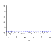
Example 3.
Figure 3 (a) presents the theoretical autocovariance function of the process , where is a FIEGARCH process, with the same parameter values considered in Figures 1 and 4. Figure 3 (b) shows the sample autocovariance function of the time series , where is the simulated time series presented in Figure 1. Figure 3 (c) presents the sample autocovariance function of the time series , where is the Bovespa index log-returns time series (see Section 5). By comparing the three graphs in Figure 3, one concludes that all three functions present a similar behavior. Since the sample autocovariance function is an estimator of the theoretical autocovariance function, it is expected that their graphics will have the same behavior. The similarity between the decay in the graphs in Figure 3 (b) and (c) indicates that a FIEGARCH model seems appropriate for fitting the Bovespa index log-returns time series.
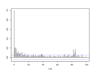
Example 4.
Theorem 4 provides the expression for the autocorrelation function of . The spectral density function of the process is given by (see [29])
where is given in (11), , is the real part of and . As an illustration, Figure 4 (a) shows the spectral density function of the process , where is any FIEGARCH process with , , , and , assuming (dashed line) and (continuous line). The corresponding values of , and , used in the computation of , are given in Table 1. Figure 4 (b) shows the periodogram function of the time series , where is the simulated time series presented in Figure 1 (a), with . Figure 4 (c) shows the periodogram function of the time series , where is the Bovespa index log-returns time series.
| Distribution | ||||||||
|---|---|---|---|---|---|---|---|---|
| 0.7979 | 0.0925 | -1.2704 | 4.9348 | 0.0559 | 0.3088 | |||
| GED | 0.7674 | 0.0975 | -1.4545 | 5.4469 | 0.0596 | 0.3389 |
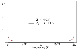


Figure 4 (a) indicates that the probability distribution of may not be evident from the periodogram function given the similarity between the graphs of . The small difference on the values of for and is explained by the fact that the values of , and are relatively close for and as shown in Table 1. Moreover, one observes that the graphs in Figure 4 (b) and (c) present similar behavior, indicating that a FIEGARCH model may be adequate to fit the data. On the other hand, Figure 4 (a) shows evidence that the underlying probability distribution of may not be the same as . In fact, we apply the two-sample Kolmogorov-Smirnov test to verify the hypothesis that and have the same probability distribution. We also apply the test to the standardized versions of and (that is, we subtracted the sample mean and divided by the sample standard deviation). In the first case the test rejects the null hypothesis (, test statistic = 0.2208, ). In the second case (standardized version) the test did not reject the null hypothesis (, test statistic = 0.0285, ).
To further investigate whether the correct probability distribution of can be identified through the periodogram function we consider the same time series as in Figure 4 (b) and perform the Kolmogorov-Smirnov hypothesis test as described in [25], pages 339 - 342, considering both cases and . Recall that
-
•
the null hypothesis of the test is that has spectral density function ;
-
•
the testing procedure consists on ploting the Kolmogorov-Smirnov boundaries
and the function defined as
with , and
where is the integer part of and is the time series sample size;
-
•
the null hypothesis is rejected if exits the boundaries for some .
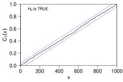
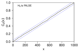

The results of the tests are given in Figure 5, where and denote the values of obtained, respectively, when assuming and . From Figures 5 (a) and (b) one concludes that the Kolmogorov-Smirnov test does not reject the null hypothesis in both cases. This result was expected given the small difference between the values of , shown in Figure 4 (a). In fact, by comparing Figures 5 (a) and (b), one observes no visible difference between those graphs. Figure 5 (c) confirms that the difference is too small to be noticed since , for all . This shows that, for the FIEGARCH process considered in Example 4, the correct probability distribution of cannot be identified through the periodogram function, given that the Kolmogorov-Smirnov hypothesis test failed to reject the null hypothesis when it was false.
To conclude this section we present the following theorem which shows that, under mild conditions, is an ARFIMA process with correlated innovations. This results is very useful in model identification and parameter estimation since the literature of ARFIMA models is well developed (see [15] and references therein).
Theorem 5.
Proof.
Let be a FIEGARCH process. From expressions (6) and (7) we have
where
In particular, if , we have and , for all .
Now, suppose that . Since is a sequence of i.i.d. random variables and , one concludes that , for all . Therefore, and . Consequently, , for all .
Let be defined by expression (28). Assume, for the moment, that , for all . It follows that
| (29) |
Since is a white noise process we have
which does not depend on . From the independence of the random variables , for all , one has
and
where does not depend on . Also, from the independence of the random variables , for all , we have
which does not depend on .
Therefore, all four terms in expression (29) do not depend on and expression (27) holds. Now, to validate expression (27) we only need to show that , for all . Notice that, since , it follows that . Upon replacing in (29) one obtains
By hypothesis, and . It follows that and . We also know that . In order to show that , notice that and, since and , from Hölder’s inequality, we have and . Then from (8) it follows that
where . By using the fact that , for all , one concludes that
Hence and, consequently, and . Therefore, the result follows. ∎
3 Forecasting
Let be a FIEGARCH process, given in Definition 1, and a time series obtained from this process. In this section, we prove that is a martingale difference with respect to the filtration , where , and we provide the -step ahead forecast for the process . Since the process , defined by (7), has an ARFIMA representation, the -step ahead forecasting for this process and its mean square error value can be easily obtained (for instance, see [15] and [31]). This fact is used to provide an -step ahead forecast for and the mean square error of forecasting. We also consider the fact that , for all , to provide an -step ahead forecast for both processes, and , based on the predictions obtained from the process . The notation used in this section is introduced below.
Remark 5.
Let , for , denote any random variable defined here. In the sequel we consider the following notation:
-
•
we use the symbol “^” to denote the -ahead step forecast defined in terms of the conditional expectation, that is, . Notice that this is the best linear predictor in terms of mean square error value. The symbols “~” and “ˇ” are used to denote alternative estimators (e.g. and );
-
•
for simplicity of notation, for the -step ahead forecast of , we write instead of (analogously for “~” and “ˇ”);
-
•
we follow the approach usually considered in the literature and denote the -ahead step forecast as instead of . If necessary, to avoid confusion, we will denote the square of as (analogously for “~” and “ˇ”).
The following lemma shows that a FIEGARCH process is a martingale difference with respect to . This result is useful in the proof of Lemma 2 that presents the -step ahead forecast of , for a fixed value of and all , and the -step ahead forecast of , given .
Lemma 1.
Let be a FIEGARCH process, given in Definition 1 and . Then the process is a martingale difference with respect to .
Proof.
From definition, is a -measurable function. Moreover, for all , and Therefore, the process is a martingale difference with respect to . ∎
Lemma 2.
Let be a stationary FIEGARCH process, given by Definition 1. Then, for any fixed , the -step ahead forecast of , for all and the -step ahead forecast of , given , are, respectively, and .
Proof.
From Lemma 1, a FIEGARCH process is a martingale difference. It follows that , for all . From definition, . Therefore, the -step ahead forecast of , given , is . Moreover, if , for all , then this is the best forecast value in mean square error sense. ∎
To obtain the -step ahead forecast for , notice that and are independent and so are and , for all . Moreover, , for all . It follows that
While for ARCH/GARCH models, can be easily calculated, for FIEGARCH processes, what is easy to derive is the expression for the -step ahead forecast for the process , for any . The expressions for and for the mean square error of forecast are given in Proposition 4. We shall use this result to discuss the properties of the predictor obtained by considering , for all .
Proposition 4.
Proof.
Since is a function of and is a sequence of i.i.d. random variables with zero mean and variance , we conclude that
and zero if . ∎
In practice, cannot be easily calculated for FIEGARCH models and thus, a common approach is to predict through the relation , with defined by (30), for all . As a consequence, a -step ahead forecast for is defined as and a naive estimator for is obtained by letting
| (32) |
From expressions (6) and (32), it is obvious that is a biased estimator for , whenever . Proposition 5 gives the mean square error forecast for the -step ahead forecast of , defined through expression (32).
Proposition 5.
Let , for all , be the -step ahead forecast of , given the filtration , defined by expression (32). Then the mean square error forecast is given by
Proof.
Remark 6.
If the values of and are known only for then the -step ahead forecast of , is approximated by
and, by definition, the same approximation follows for . It is easy to see that, in this case, the mean square error of forecast values for the processes and are given, respectively, by
From Jensen’s inequality, one concludes that
so that , for all . In fact, from (16) and (30), we have
| (34) |
Another -step ahead predictor for can be defined as follows. Consider an order 2 Taylor’s expansion of the exponential function and write
| (35) |
From expression (35), a natural choice is to define a -step ahead predictor for as
| (36) |
for all .
Since is a -measurable random variable, for all , we have . From equation (35), we easily conclude that, for all ,
Therefore, the relation between the bias for the estimators and is given by
In Section 4 we analyze the performance of through a Monte Carlo simulation study.
4 Simulation Study
In this section we present a Monte Carlo simulation study to analyze the performance of quasi-likelihood estimator and also the forecasting on FIEGARCH processes. Six different models are considered and, from now on, they shall be referred to as model M, for . For all models we assume that the distribution of is the Generalized Error Distribution (GED) with tail-thickness parameter (since the tails are heavier than the Gaussian distribution). The set of parameters considered in this study is the same as in [12] and [13]444[12] present a Monte Carlo simulation study on risk measures estimation in time series derived from FIEGARCH process. [13] analyze a portfolio composed by stocks from the Brazilian market Bovespa. The authors consider the econometric approach to estimate the risk measure VaR and use FIEGARCH models to obtain the conditional variance of the time series., except for models M5 and M6 (see Table 2). While model M5 considers , which is close to the non-stationary region (), model M6 considers and . For comparison, we shall consider for model M6 the same parameter values as in model M3 (obviously, with the necessary adjustments regarding and ). We also present here the step-ahead forecast, for , for the conditional variance of simulated FIEGARCH processes.
4.1 Data Generating Process
To generate samples from FIEGARCH processes we proceed as described in steps DGP1 - DGP3 below. Notice that, while step 1 only needs to be repeated for each model, steps 2 and 3 must be repeated for each model and each replication. The parameters value consider in this simulation study are given in Table 2. For each model we consider replications, with sample size .
| Model | Parameter | |||||||||
|---|---|---|---|---|---|---|---|---|---|---|
| M1 | 0.4495 | -0.1245 | 0.3662 | -6.5769 | -1.1190 | -0.7619 | -0.6195 | - | - | - |
| M2 | 0.2391 | -0.0456 | 0.3963 | -6.6278 | - | - | 0.2289 | 0.1941 | 0.4737 | -0.4441 |
| M3 | 0.4312 | -0.1095 | 0.3376 | -6.6829 | - | - | 0.5454 | - | - | - |
| M4 | 0.3578 | -0.1661 | 0.2792 | -7.2247 | - | - | 0.6860 | - | - | - |
| M5 | 0.4900 | -0.0215 | 0.3700 | -5.8927 | 0.1409 | - | -0.1611 | - | - | - |
| M6 | 0.4312 | -0.1095 | 0.3376 | -6.6829 | 0.5454 | - | - | - | - | - |
DGP1: Apply the recurrence formula given in Proposition 2, to obtain the coefficients of the polynomial , defined by (14). For this simulation study the infinite sum (14) is truncated at . To select the truncation point we consider Theorem 3 and the results presented in Table 3.
From Theorem 3, we have,
and we conclude that and , as goes to infinity. However, the speed of the convergence varies from model to model, as we show in Table 3. For simplicity, in this table, let and be defined as
Table 3 presents the values of the coefficients , given in Proposition 2, for 100; 1,000; 5,000; 10,000; 20,000; 50,000; 100,000, for each simulated model M, . Note that, for 5,000, the coefficient values decrease slowly. We also report in Table 3 and values for the correspondent value. Note that, for 10,000; 50,000; 100,000, the value is very close to zero, for all models. Also notice that, while converges to 1 faster for model M1 than for the other models.
| 0 | 10 | 100 | 1,000 | 5,000 | 10,000 | 25,000 | 50,000 | 100,000 | |
| M1 := FIEGARCH | |||||||||
| 1 | 0.26537 | 0.07167 | 0.02015 | 0.00830 | 0.00567 | 0.00342 | 0.00234 | 0.00160 | |
| - | 0.09426 | 0.00904 | 0.00090 | 0.00018 | 0.00009 | 0.00004 | 0.00002 | 0.00001 | |
| - | 1.04410 | 1.00173 | 1.00017 | 1.00003 | 1.00002 | 1.00001 | 1.00000 | 1.00000 | |
| M2 := FIEGARCH | |||||||||
| 1 | -0.09039 | 0.01450 | 0.00251 | 0.00074 | 0.00043 | 0.00022 | 0.00013 | 0.00008 | |
| - | -0.05212 | 0.00482 | 0.00048 | 0.00010 | 0.00005 | 0.00002 | 0.00001 | 0.00000 | |
| - | -1.08434 | 1.00292 | 1.00027 | 1.00005 | 1.00003 | 1.00001 | 1.00001 | 1.00000 | |
| M3 := FIEGARCH | |||||||||
| 1 | 0.31434 | 0.07844 | 0.02106 | 0.00843 | 0.00568 | 0.00337 | 0.00227 | 0.00153 | |
| - | 0.11647 | 0.01077 | 0.00107 | 0.00021 | 0.00011 | 0.00004 | 0.00002 | 0.00001 | |
| - | 1.08789 | 1.00576 | 1.00056 | 1.00011 | 1.00006 | 1.00002 | 1.00001 | 1.00001 | |
| M4 := FIEGARCH | |||||||||
| 1 | 0.36874 | 0.06738 | 0.01517 | 0.00539 | 0.00345 | 0.00192 | 0.00123 | 0.00079 | |
| - | 0.16178 | 0.01297 | 0.00128 | 0.00026 | 0.00013 | 0.00005 | 0.00003 | 0.00001 | |
| - | 1.26414 | 1.01350 | 1.00129 | 1.00026 | 1.00013 | 1.00005 | 1.00003 | 1.00001 | |
| M5 := FIEGARCH | |||||||||
| 1 | 0.12291 | 0.03897 | 0.01207 | 0.00531 | 0.00373 | 0.00234 | 0.00164 | 0.00115 | |
| - | 0.03977 | 0.00408 | 0.00041 | 0.00008 | 0.00004 | 0.00002 | 0.00001 | 0.00000 | |
| - | 0.97189 | 0.99720 | 0.99972 | 0.99994 | 0.99997 | 0.99999 | 0.99999 | 1.00000 | |
| M6 := FIEGARCH | |||||||||
| 1 | 0.05472 | 0.01599 | 0.00435 | 0.00174 | 0.00117 | 0.00070 | 0.00047 | 0.00032 | |
| - | 0.02027 | 0.00219 | 0.00022 | 0.00004 | 0.00002 | 0.00001 | 0.00000 | 0.00000 | |
| - | 0.91632 | 0.99192 | 0.99919 | 0.99984 | 0.99992 | 0.99997 | 0.99998 | 0.99999 | |
DGP2: Set , with , and obtain an i.i.d. sample .
DGP3: By considering Definition 1 and the equality in (14), the sample is obtained through the relation
Remark 7.
For parameter estimation and forecasting we shall consider sub-samples from these time series, with size . The sub-samples of size correspond to the last 2,000 values of the generated time series (after removing the last 50 values which are used only to compare the out-of-sample forecasting performance of the models). The value is the approximated size of the observed time series considered in [13]. The value was chosen to analyze the estimators asymptotic properties.
4.2 Estimation Procedure
In this study we consider the quasi-likelihood method to estimate the parameters of FIEGARCH models for the simulated time series. Given any time series , this method assumes that , for all , is normally distributed. The vector of unknown parameters is denoted by
and the estimator of is the value that maximizes
| (38) |
Since the processes and are unknown, we need to consider a set of initial conditions in order to start the recursion and to obtain the random variable , for . Then we use these estimated values to solve (38). For this simulation study we assume, as initial conditions, , and , whenever , where is the sample variance of . This is the initial set suggested by [6]. The random variables , for , are then estimated upon considering the set of initial conditions and the known values . The infinite sum in the polynomial is truncated at , where is the available sample size.
4.3 Performance Measures
For any model, let denotes the estimate of in the -th replication, where , and is any vector parameter given in Table 2. To access the performance of quasi-likelihood procedure we calculate the mean , the standard deviation (), the bias (), the mean absolute error () and the mean square error () values, defined by
where , for .
4.4 Estimation Results
Table 4 summarizes the results on the parameter estimation procedure. Figures 6 - 11 present the kernel distribution of the parameter estimators for each considered model when . These graphs help to illustrate the results presented in Table 4.
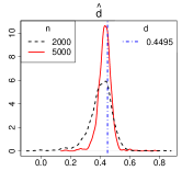
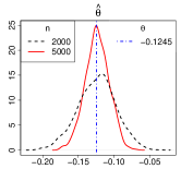
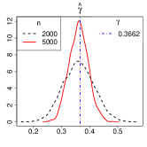
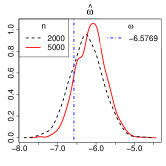
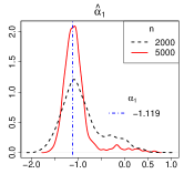
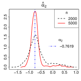
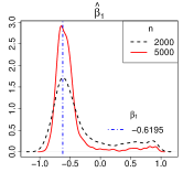
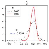
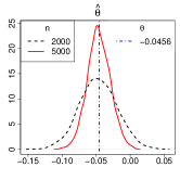
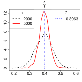
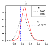
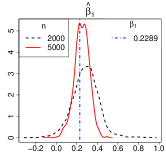
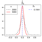
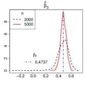
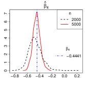
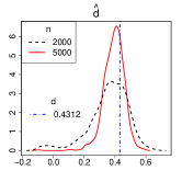
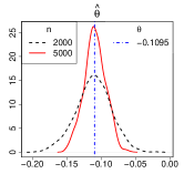
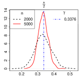
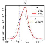
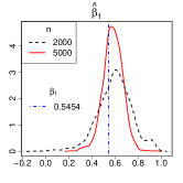
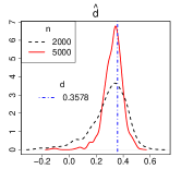
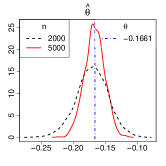
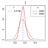
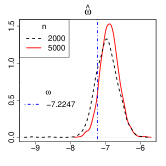
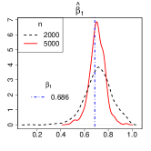
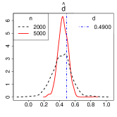
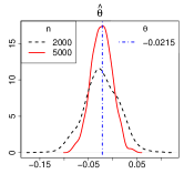
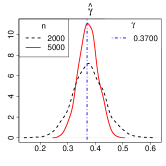
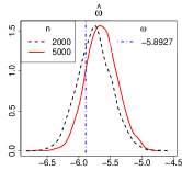
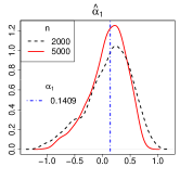
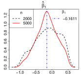
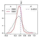
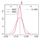
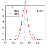
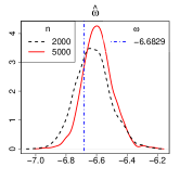
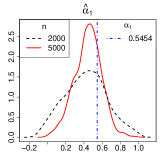
By observing Figures 6 - 11, it is easy to see that, for most estimates, the density function is approximately symmetric. For some parameters, we notice the presence of possible outliers, see for instance the graphs for the parameters (in particular, models M2, M3 and M4), (model M2) and (in particular, models M1 and M2), with and . Although the graphs for and are similar, one observes that, as expected, the observations tend to concentrate closer to the mean when .
| Sample Size () | |||||||||||
|---|---|---|---|---|---|---|---|---|---|---|---|
| Parameter () | |||||||||||
| M1 := FIEGARCH; | |||||||||||
| 0.4495 () | 0.4022 | 0.0854 | -0.0473 | 0.0688 | 0.0095 | 0.4309 | 0.0468 | -0.0186 | 0.0357 | 0.0025 | |
| -0.1245 () | -0.1240 | 0.0266 | 0.0005 | 0.0213 | 0.0007 | -0.1237 | 0.0168 | 0.0008 | 0.0133 | 0.0003 | |
| 0.3662 () | 0.3612 | 0.0543 | -0.0050 | 0.0438 | 0.0030 | 0.3610 | 0.0337 | -0.0052 | 0.0271 | 0.0012 | |
| -6.5769 () | -6.2516 | 0.4270 | 0.3253 | 0.4358 | 0.2881 | -6.1284 | 0.3830 | 0.4485 | 0.4930 | 0.3479 | |
| -1.1190 () | -0.9067 | 0.4519 | 0.2123 | 0.3567 | 0.2492 | -1.0344 | 0.3259 | 0.0846 | 0.2010 | 0.1134 | |
| -0.7619 () | -0.6517 | 0.4035 | 0.1102 | 0.2832 | 0.1750 | -0.7281 | 0.2623 | 0.0338 | 0.1534 | 0.0700 | |
| -0.6195 () | -0.3415 | 0.4774 | 0.2780 | 0.3474 | 0.3052 | -0.5052 | 0.3214 | 0.1143 | 0.1764 | 0.1164 | |
| M2 := FIEGARCH; | |||||||||||
| 0.2391 () | 0.1683 | 0.1538 | -0.0708 | 0.1216 | 0.0287 | 0.2077 | 0.0767 | -0.0314 | 0.0650 | 0.0069 | |
| -0.0456 () | -0.0469 | 0.0275 | -0.0013 | 0.0220 | 0.0008 | -0.0461 | 0.0169 | -0.0005 | 0.0134 | 0.0003 | |
| 0.3963 () | 0.3931 | 0.0536 | -0.0032 | 0.0426 | 0.0029 | 0.3959 | 0.0326 | -0.0004 | 0.0256 | 0.0011 | |
| -6.6278 () | -6.5525 | 0.1146 | 0.0753 | 0.1075 | 0.0188 | -6.5077 | 0.0905 | 0.1201 | 0.1253 | 0.0226 | |
| 0.2289 () | 0.2841 | 0.1284 | 0.0552 | 0.1083 | 0.0195 | 0.2488 | 0.0721 | 0.0199 | 0.0593 | 0.0056 | |
| 0.1941 () | 0.2078 | 0.0865 | 0.0137 | 0.0657 | 0.0077 | 0.1990 | 0.0456 | 0.0049 | 0.0367 | 0.0021 | |
| 0.4737 () | 0.4710 | 0.0935 | -0.0027 | 0.0667 | 0.0088 | 0.4784 | 0.0441 | 0.0047 | 0.0349 | 0.0020 | |
| -0.4441 () | -0.4704 | 0.1063 | -0.0263 | 0.0867 | 0.0120 | -0.4500 | 0.0592 | -0.0059 | 0.0466 | 0.0035 | |
| M3 := FIEGARCH; | |||||||||||
| 0.4312 () | 0.3606 | 0.1268 | -0.0706 | 0.1043 | 0.0211 | 0.3933 | 0.0648 | -0.0379 | 0.0569 | 0.0056 | |
| -0.1095 () | -0.1111 | 0.0255 | -0.0016 | 0.0201 | 0.0007 | -0.1090 | 0.0157 | 0.0005 | 0.0125 | 0.0002 | |
| 0.3376 () | 0.3346 | 0.0493 | -0.0030 | 0.0394 | 0.0024 | 0.3331 | 0.0300 | -0.0045 | 0.0241 | 0.0009 | |
| -6.6829 () | -6.3686 | 0.4230 | 0.3143 | 0.4271 | 0.2778 | -6.2413 | 0.3715 | 0.4416 | 0.4814 | 0.3330 | |
| 0.5454 () | 0.5976 | 0.1472 | 0.0522 | 0.1231 | 0.0244 | 0.5822 | 0.0851 | 0.0368 | 0.0731 | 0.0086 | |
| M4 := FIEGARCH; | |||||||||||
| 0.3578 () | 0.2950 | 0.1338 | -0.0628 | 0.1056 | 0.0218 | 0.3258 | 0.0721 | -0.0320 | 0.0569 | 0.0062 | |
| -0.1661 () | -0.1702 | 0.0248 | -0.0041 | 0.0198 | 0.0006 | -0.1666 | 0.0156 | -0.0005 | 0.0124 | 0.0002 | |
| 0.2792 () | 0.2793 | 0.0415 | 0.0001 | 0.0326 | 0.0017 | 0.2769 | 0.0248 | -0.0023 | 0.0197 | 0.0006 | |
| -7.2247 () | -6.9615 | 0.3122 | 0.2632 | 0.3284 | 0.1667 | -6.8766 | 0.2604 | 0.3481 | 0.3689 | 0.1889 | |
| 0.6860 () | 0.7160 | 0.1128 | 0.0300 | 0.0915 | 0.0136 | 0.7067 | 0.0665 | 0.0207 | 0.0535 | 0.0048 | |
| M5 := FIEGARCH; | |||||||||||
| 0.4900 () | 0.4258 | 0.1273 | -0.0642 | 0.1096 | 0.0203 | 0.4453 | 0.0645 | -0.0447 | 0.0629 | 0.0062 | |
| -0.0215 () | -0.0229 | 0.0355 | -0.0014 | 0.0282 | 0.0013 | -0.0229 | 0.0218 | -0.0014 | 0.0175 | 0.0005 | |
| 0.3700 () | 0.3751 | 0.0577 | 0.0051 | 0.0455 | 0.0034 | 0.3742 | 0.0354 | 0.0042 | 0.0285 | 0.0013 | |
| -5.8927 () | -5.7507 | 0.2688 | 0.1420 | 0.2415 | 0.0924 | -5.6414 | 0.2494 | 0.2513 | 0.2902 | 0.1253 | |
| 0.1409 () | 0.1152 | 0.4082 | -0.0257 | 0.3232 | 0.1673 | 0.1012 | 0.3310 | -0.0397 | 0.2613 | 0.1111 | |
| -0.1611 () | -0.1383 | 0.3799 | 0.0228 | 0.3189 | 0.1448 | -0.1581 | 0.3213 | 0.0030 | 0.2579 | 0.1032 | |
| M6 := FIEGARCH; | |||||||||||
| 0.4312 () | 0.3220 | 0.1825 | -0.1092 | 0.1706 | 0.0452 | 0.3449 | 0.1135 | -0.0863 | 0.1107 | 0.0203 | |
| -0.1095 () | -0.1132 | 0.0351 | -0.0037 | 0.0282 | 0.0012 | -0.1114 | 0.0222 | -0.0019 | 0.0176 | 0.0005 | |
| 0.3376 () | 0.3368 | 0.0585 | -0.0008 | 0.0467 | 0.0034 | 0.3380 | 0.0355 | 0.0004 | 0.0283 | 0.0013 | |
| -6.6829 () | -6.6233 | 0.1144 | 0.0596 | 0.1014 | 0.0166 | -6.5926 | 0.0978 | 0.0903 | 0.1071 | 0.0177 | |
| 0.5454 () | 0.4189 | 0.2297 | -0.1265 | 0.2109 | 0.0688 | 0.4429 | 0.1492 | -0.1025 | 0.1428 | 0.0328 | |
From Table 4 we conclude that, given the models complexity, the quasi-likelihood method performs relatively well. Since model M2 presents more parameters than the other models, which implies a higher dimension maximization problem, one would expect that the quasi-likelihood method would present the worst performance in this case. However, in terms of or values, the estimation results for model M2 (, and ), M3 (, and ), M4 (, and ) and M6 (, and ) are similar (except for the parameter in model M6) and the quasi-likelihood method performs better for model M2 (except for the parameter ) than for models M1 (, and ) and M5 (, and ).
Table 4 also indicates that the quasi-likelihood procedure may perform better for and than for and (we shall investigate this in a future work). This conclusion is based on the fact that models M3 and M6 have the same parameter values (with the necessary adjustments in and ) and all parameters, except , were better estimated in model M3 than M6.
By comparing the and values, given in Table 4, we conclude that the worst performance occurs for models M1 and M5 (in particular, see the estimation results for , and , and ). This outcome is explained by the fact that the parameter is very close to the non-stationary region for model M5 and, for model M1, not only but also , which implies a more complex model with stronger long-range dependence. The small values indicate that, for all parameters, the mean estimated value is very close to the true value. Although for the standard deviation of several estimates is high if compared with the mean estimated value, as expected, the estimators performance improves as the sample size increases.
4.5 Forecasting Procedure
To obtain the predicted values, for each replication of model M, with , and each sub-sample , with , we repeat steps F1 - F5 below.
F1: Replace the true parameters values by the estimated ones, namely, , and use the recurrence formula given in Proposition 2 to calculate the corresponding coefficients .
F2: Obtain the time series (which corresponds to the residuals of the fitted model) and . To do so, let , whenever , and calculate and recursively as follows:
for all .
F3: In expression (11), replace and by their respective sample estimates, and obtain an estimate for given by
F5: Based on the fact that , set , for all .
4.6 Forecasting Results
In what follows we discuss the simulation results related to forecasting based on the fitted FIEGARCH models. To access the models forecast performance, during the generating process, we create 50 extra values for each simulated time series. Those values are used here to compare with the -step ahead forecast, for .
Table 5 presents the mean over simulated values of and obtained from model M, for each , and the corresponding -step ahead predicted values , for , forecasting origin and sub-samples . This table also reports the mean square error () of forecast, defined as
where is the number of replications, denotes the true value of (or ) and is the predicted value obtained in the -th replication, for , based on the model fitted to the sub-sample with size . Notice that, due to the small magnitude of the sample means, all values in Table 5 are multiplied by 100.
| 2,000 | 5,000 | |||||||||
| Predictor | Predictor | |||||||||
| M1 := FIEGARCH; | ||||||||||
| 1 | 0.1698 | 0.1575 | 0.1652 | 0.0010 | 0.0993 | 0.1634 | 0.0003 | 0.0969 | ||
| 2 | 0.1635 | 0.1473 | 0.1640 | 0.0038 | 0.0900 | 0.1611 | 0.0032 | 0.0875 | ||
| 3 | 0.1636 | 0.1540 | 0.1655 | 0.0078 | 0.1122 | 0.1632 | 0.0075 | 0.1116 | ||
| 4 | 0.1629 | 0.1490 | 0.1662 | 0.0122 | 0.1117 | 0.1633 | 0.0114 | 0.1101 | ||
| 5 | 0.1641 | 0.1542 | 0.1665 | 0.0147 | 0.1906 | 0.1642 | 0.0141 | 0.1903 | ||
| M2 := FIEGARCH; | ||||||||||
| 1 | 0.1387 | 0.1284 | 0.1359 | 0.0004 | 0.0521 | 0.1369 | 0.0002 | 0.0515 | ||
| 2 | 0.1383 | 0.1246 | 0.1395 | 0.0024 | 0.0506 | 0.1398 | 0.0021 | 0.0501 | ||
| 3 | 0.1357 | 0.1299 | 0.1374 | 0.0027 | 0.0551 | 0.1381 | 0.0024 | 0.0547 | ||
| 4 | 0.1378 | 0.1276 | 0.1390 | 0.0029 | 0.0562 | 0.1399 | 0.0028 | 0.0559 | ||
| 5 | 0.1356 | 0.1253 | 0.1409 | 0.0036 | 0.0568 | 0.1414 | 0.0034 | 0.0570 | ||
| M3 := FIEGARCH; | ||||||||||
| 1 | 0.1487 | 0.1380 | 0.1452 | 0.0007 | 0.0833 | 0.1439 | 0.0002 | 0.0848 | ||
| 2 | 0.1456 | 0.1287 | 0.1459 | 0.0026 | 0.0681 | 0.1442 | 0.0022 | 0.0674 | ||
| 3 | 0.1426 | 0.1350 | 0.1466 | 0.0052 | 0.0773 | 0.1447 | 0.0045 | 0.0777 | ||
| 4 | 0.1438 | 0.1200 | 0.1473 | 0.0075 | 0.0619 | 0.1453 | 0.0068 | 0.0600 | ||
| 5 | 0.1411 | 0.1354 | 0.1479 | 0.0076 | 0.1316 | 0.1459 | 0.0069 | 0.1309 | ||
| M4 := FIEGARCH; | ||||||||||
| 1 | 0.0932 | 0.0894 | 0.0918 | 0.0005 | 0.0411 | 0.0910 | 0.0002 | 0.0416 | ||
| 2 | 0.0905 | 0.0809 | 0.0918 | 0.0013 | 0.0275 | 0.0908 | 0.0010 | 0.0270 | ||
| 3 | 0.0885 | 0.0810 | 0.0917 | 0.0027 | 0.0293 | 0.0907 | 0.0022 | 0.0291 | ||
| 4 | 0.0886 | 0.0764 | 0.0918 | 0.0040 | 0.0251 | 0.0908 | 0.0036 | 0.0242 | ||
| 5 | 0.0876 | 0.0831 | 0.0919 | 0.0042 | 0.0461 | 0.0909 | 0.0037 | 0.0456 | ||
| M5 := FIEGARCH; | ||||||||||
| 1 | 0.2898 | 0.2669 | 0.2808 | 0.0012 | 0.2096 | 0.2795 | 0.0005 | 0.2087 | ||
| 2 | 0.2883 | 0.2800 | 0.2833 | 0.0069 | 0.2489 | 0.2817 | 0.0065 | 0.2494 | ||
| 3 | 0.2908 | 0.2836 | 0.2844 | 0.0081 | 0.2452 | 0.2821 | 0.0081 | 0.2461 | ||
| 4 | 0.2909 | 0.2963 | 0.2847 | 0.0077 | 0.3178 | 0.2827 | 0.0076 | 0.3174 | ||
| 5 | 0.2923 | 0.2971 | 0.2852 | 0.0097 | 0.3695 | 0.2832 | 0.0096 | 0.3704 | ||
| M6 := FIEGARCH; | ||||||||||
| 1 | 0.1271 | 0.1143 | 0.1242 | 0.0001 | 0.0367 | 0.1247 | 0.0001 | 0.0367 | ||
| 2 | 0.1260 | 0.1140 | 0.1265 | 0.0013 | 0.0379 | 0.1265 | 0.0013 | 0.0377 | ||
| 3 | 0.1259 | 0.1228 | 0.1262 | 0.0014 | 0.0471 | 0.1263 | 0.0013 | 0.0471 | ||
| 4 | 0.1284 | 0.1188 | 0.1263 | 0.0018 | 0.0479 | 0.1264 | 0.0017 | 0.0477 | ||
| 5 | 0.1261 | 0.1192 | 0.1264 | 0.0015 | 0.0473 | 0.1265 | 0.0014 | 0.0474 | ||
From Table 5 (see also Figure 12 below) conclude that,
-
•
when we consider , the predicted values are relatively close to the simulated ones, which is indicated by the small values, for all models and any ;
- •
-
•
when we consider , the is usually high, if compared to the mean simulated and mean predicted values. Therefore, we conclude that is a poor estimator for . This result is not a surprise since the main purpose of FIEGARCH models is to estimate the logarithm of the conditinal variance of the process and not the process itself;
-
•
as expected, in all cases, the models’ forecasting performance improves as increases. Notice, however, that the difference in the values, from to , is small (recall that the values are multiplied by 100). This is so because the coefficients converges to zero, as goes to infinity. Therefore, it is expected that, for some and any , using the last or the last known values to calculate the -step ahead forecast value for the process will not considerably change the results.
Figure 12 shows the mean taken over 1,000 replications for:
-
•
the simulated values and obtained from model M, for each , and ;
-
•
the one-step ahead forecast values (denoted in the graphs by ), for , and . The predictor is obtained directly from the sub-sample , by following steps F1 -F5 (this figure only reports the graphs for the case ). The remaining predicted values are calculated by updating the forecasting origin from to , that is, by introducing the observations , one at a time, and following steps F2 -F5;
-
•
the -step ahead forecast values considering the predictors and (denoted in the graphs by ). These values are obtained by following steps F1 -F5 with forecasting origin (without update). For all graphs the size of the sub-sample used for parameter estimation and forecasting is .
The dashed lines in Figure 12 correspond to the limiting constants and , for , described in the sequel.
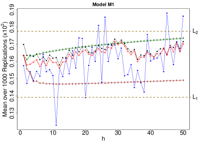
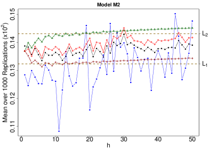
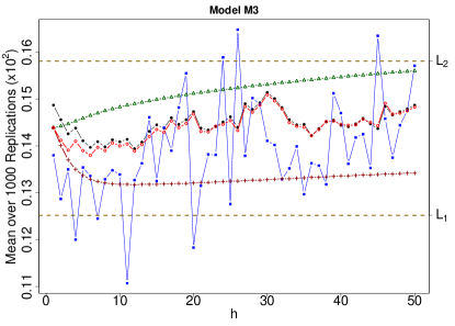
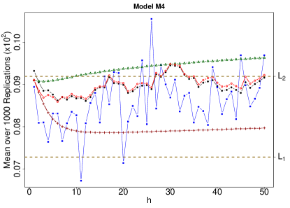
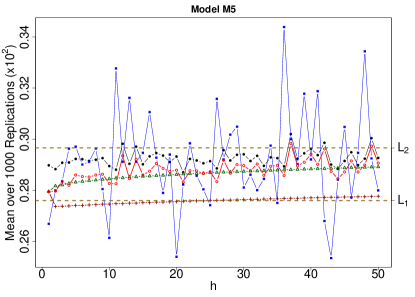
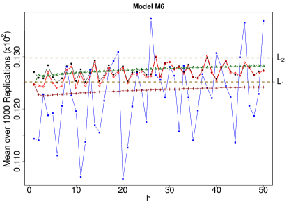
From Figure 12 we observe that, for all models, the means for the one-step ahead forecast values , show the same behavior over the time as the means for the true values , where , and . As expected, due to the error carried from the parameter estimation (specially, from the distribution misspecification), we observe a small forecasting bias, which decreases as increases. The decrease in the forecasting bias, as the forecasting origin is updated, can be attributed to the fact that we start the recurrence formula (step F2) assuming and as the new observations are introduced, the constant is replaced by its sample estimate (step F3), which provides more accurate values for as increases ().
Regarding the -step ahead predictors and , Figure 12 shows that the estimation bias is higher if we consider the former one. This figure also shows that, for all models, the predicted value converges to a constant as increases. This is expected since the -step ahead predictor is defined in terms of the conditional expectation. In fact, from expression (34), converges to as goes to infinity, where denotes the parameter for model M and hence, from expression (37),
| (39) |
for each and sufficiently large. The values of (also given in Table 2), and , for and , are presented in Table 6.
| 1 | 2 | 3 | 4 | 5 | 6 | |
|---|---|---|---|---|---|---|
| -6.5769 | -6.6278 | -6.6829 | -7.2247 | -5.8927 | -6.6829 | |
| 0.1392 | 0.1323 | 0.1252 | 0.0728 | 0.2760 | 0.1252 | |
| 0.1775 | 0.1431 | 0.1581 | 0.0919 | 0.2966 | 0.1298 |
Upon comparing the values of and , given in Table 6 (also reported in Figure 12 as and ), for each , respectively, with the limits and (see Figure 12), we conclude that these values are close to each other, for all models. A small difference between and (respectively, and ) is expected since the former one is calculated using the true parameter values while is obtained by considering the estimates for the parameter.
5 Analysis of an Observed Time Series
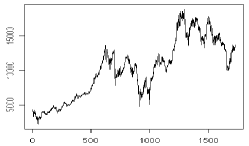
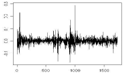
This section presents the analysis of the São Paulo Stock Exchange Index (Bovespa Index or IBovespa) log-return time series. We consider the FIEGARCH model, fully described in this paper, and we compare its forecasting performance with other ARCH-type models. The total number of observations for the IBovespa time series is . We consider the first 1717 observations to fit the models and we reserve the last 20 ones to compare with the out-of-sample forecast.
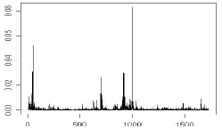
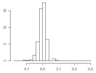
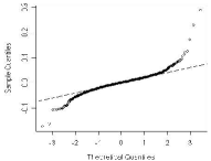
Figure 13 (a) presents IBovespa time series , in the period of January/1995 to December/2001. We observe a strong decay in the index value close to (that is, January 15, 1999). This period is characterized by the Real (the Brazilian currency) devaluation. Figures 13 (b) and (c) present, respectively, the IBovespa log-return time series, , and the square of the log-return time series, , in the same period. Observe that the log-return series presents the stylized facts of financial time series such as apparent stationarity, mean around zero and clusters of volatility. Also, in Figure 14 we observe that, while the log-return series presents almost no correlation, the sample autocorrelation of the square of the log-return series assumes high values for several lags, pointing to the existence of heteroskedasticity and possibly long memory. Notice that the periodogram of , presented in Figure 4 (c), also indicates possibly long-memory in the conditional variance. Regarding the histogram and the QQ-Plot, we observe that the distribution of the log-return series seems approximately symmetric and leptokurtic.
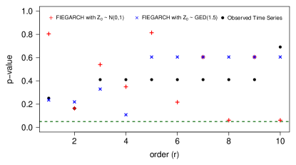
To investigate whether the stationarity property holds for the time series we apply the runs test (or Wald-Wolfwitz test), as described in [32]. Due to the magnitude of the data we multiply the time series values by 100 before applying the test. The p-values for the test considering the moments of order555For the values of are too close to zero and the test always returns the same p-value as . are reported in Figure 15. For comparison, this figure also shows the p-values of the test applied to the simulated time series presented in Figure 1. Notice that, for all the test does not reject the null hypothesis of stationarity.
To analyze if the ergodicity property holds for the time series we perform the test described in [33]. For comparison, we also apply this test to the simulated time series (only for sample size ) considered in Section 4. The test results are given in Table 7. The reported values are the proportion of p-values smaller than 0.05 and 0.10 in a total of 100 repetitions of step 3 of the Algorithm 1 given in [33]. Moreover, for the simulated time series, the values in Table 7 correspond to the mean taken over 1,000 replications. Notice that the proportion of p-values smaller than 0.05 (equivalently, 0.10) is always higher for the simulated time series (known to be ergodic) then for the observed time series. Given that the proportion of p-values smaller than 0.05 and 0.10 is close to the expected, we conclude that the ergodicity property holds for .
| p-values | M1 | M2 | M3 | M4 | M5 | M6 | |
|---|---|---|---|---|---|---|---|
| 0.05 | 0.10 | 0.08 | 0.09 | 0.09 | 0.07 | 0.07 | 0.05 |
| 0.10 | 0.17 | 0.13 | 0.14 | 0.15 | 0.13 | 0.12 | 0.11 |
The analysis of the sample autocorrelation function suggests an ARMA-FIEGARCH model. While an ARMA model accounts for the correlation among the log-returns, a FIEGARCH model take into account the long memory (in the conditional variance) and the heteroskedasticity characteristics of the time series. To select the best ARMA-FIEGARCH model for the data we initially considered all possible models with and and applied the quasi-likelihood method to estimate the unknown parameters. Then we eliminate the models with correlated residuals and selected the best models, with respect to the log-likelihood, Bayesian (BIC), Akaike (AIC) and Hannan-Quinn (HQC) information criteria (in this step three models were selected). The models order and the corresponding AIC, BIC and HQC values are reported in Table 8. Boldface indicates that the model was the best with respect to the corresponding the criterion.
| Order | Criterion | |||||||
|---|---|---|---|---|---|---|---|---|
| Log-likelihood | BIC | AIC | HQC | |||||
| 3 | 2 | 1 | 0.3651 | 1 | 4142.260 | -8202.588 | -8262.520 | -8240.344 |
| 0 | 1 | 0 | 0.3578 | 1 | 4138.552 | -8232.414 | -8265.104 | -8253.008 |
| 0 | 2 | 0 | 0.3785 | 1 | 4141.197 | -8230.256 | -8268.394 | -8254.282 |
Note: Boldface indicates that the model was the best, among all combinations of and , with respect to the corresponding criterion.
As shown in Table 8, the values of the selection criteria did not vary much amongst the tested models so we choose the most parsimonious one, namely, ARMA(0,1)-FIEGARCH. We compare the forecasting performance of this model with other ARCH-type models and with a radial basis function model. For this comparison the order of the ARMA part of the model was not changed, that is, we fixed and for all ARCH-type models. The EGARCH model was set to have the same values for and as the FIEGARCH model so we could investigate the influence of the long memory parameter . For the GARCH() model we choose the smallest values of and for which the residuals of the model are not correlated. The same was done for the ARCH model (which resulted in ). The ARCH(1) model was presented only for comparison. The estimated coefficients for the ARCH-type models are given in Table 9, with the corresponding log-likelihood value. Notice that, the FIEGARCH model fitted to this time series present the same parameters values as model M4 considered in the simulated study in Section 4.
| Estimate | ARMA(0,1) + | ARMA(0,1) + | ARMA(0,1) + | ARMA(0,1) + | ARMA(0,1) + |
|---|---|---|---|---|---|
| ARCH(1) | ARCH(6) | GARCH(1,1) | EGARCH(0,1) | FIEGARCH(0,,1) | |
| -0.1138 (0.0200) | -0.0642 (0.0267) | -0.0647 (0.0266) | -0.0751 (0.0254) | -0.0776 (0.0257) | |
| 0.0004 (0.0000) | 0.0002 (0.0000) | 0.0000 (0.0000) | -7.4694 (0.0969) | -7.2247 (0.2143) | |
| 0.6071 (0.0581) | 0.2307 (0.0417) | 0.2019 (0.0247) | - | - | |
| - | 0.1540 (0.0333) | - | - | - | |
| - | 0.1852 (0.0390) | - | - | - | |
| - | 0.1145 (0.0348) | - | - | - | |
| - | 0.0641 (0.0290) | - | - | - | |
| - | 0.0635 (0.0257) | - | - | - | |
| - | - | 0.7659 (0.0271) | 0.9373 (0.0103) | 0.6860 (0.0986) | |
| - | - | - | - | 0.3578 (0.0810) | |
| - | - | - | -0.1653 (0.0197) | -0.1661 (0.0224) | |
| - | - | - | 0.2782 (0.0300) | 0.2972 (0.0332) | |
| log-likelihood | 3934.337 | 4060.372 | 4072.622 | 4137.625 | 4138.552 |
| BIC | -7846.329 | -8061.157 | -8115.451 | -8238.008 | -8232.414 |
| AIC | -7862.674 | -8104.744 | -8137.244 | -8265.250 | -8265.104 |
| HQC | -7856.626 | -8088.616 | -8129.180 | -8255.170 | -8253.008 |
To fit a radial basis model to the data (no exogenous variables are considered) we assume that can be written as (see [34], [35])
with , for some , , and . Under these assumptions, and , for all . Therefore, we use neural networks and to approximate, respectively, and , and obtain
where
with , for all . In both cases, we consider one hidden layer containing neurons, for some , that is,
with , , , , the Euclidean norm, and , for any and .
To obtain a -step ahead predictor for given , we observe that, for all ,
Therefore, , for some . Thus, once and are estimated, the predictors and can be obtained recursively as
where , with , whenever .
Tables 10 and 11 present some statistics to access the out-of-sample forecasting performance, respectively, of ARCH-type and radial basis models. The values in these tables correspond to the mean absolute error (), the mean percentage error () and the maximum absolute error () of forecast, respectively defined as
where, , for and , is the -step ahead forecast error. Note that, when considering the ARMA combined with ARCH-type models, from the ARMA(0,1) part of the models, , where , for all . Since we define and is -measurable, for all , by elementary calculations we conclude that, and , for all , with . For EGARCH and FIEGARCH models, is replaced by , given in expression (36), and , where is defined in Proposition 4.
| Model | ARMA(0,1) + | ARMA(0,1) + | ARMA(0,1) + | ARMA(0,1) + | ARMA(0,1) + | ||
|---|---|---|---|---|---|---|---|
| ARCH(1) | ARCH(6) | GARCH(1,1) | EGARCH(1,1) | FIEGARCH(1,,1) | |||
| Predictor | |||||||
| 0.00053 | 0.00045 | 0.00043 | 0.00045 | 0.00044 | 0.00045 | 0.00043 | |
| 109.40844 | 68.97817 | 60.29677 | 71.33057 | 61.26625 | 68.42884 | 59.88066 | |
| 0.00094 | 0.00094 | 0.00094 | 0.00082 | 0.00087 | 0.00084 | 0.00088 | |
| Note: The high values are due to 5 observations close to zero. | |||||||
From Table 10 we conclude that, given its high value, the ARMA(0,1)-ARCH(1) does not fit the data well. In fact, the square of the residuals from this model are still correlated and we use the model only for comparison. The ARMA(0,1)-ARCH(6) model performed similar to the ARMA(0,1)-GARCH(1,1) model, in terms of both, and values, presenting a higher value. However, the latter is more parsimonious. Although the log-likelihood value is higher (and the value is smaller) for the ARMA(0,1)-EGARCH(0,1) model, the and the values are smaller for the ARMA(0,1)-GARCH(0,d,1) model. Overall, the ARMA(0,1)-FIEGARCH(0,d,1) performs slightly better than the other models.
The fact that all models present a similar perfomance confirms the following, already known in the literature.
-
•
In practice, ARCH models perform relatively well for most applications.
-
•
GARCH models are more parsimonious than the ARCH ones. For instance, notice that similar results were obtained here by considering an ARCH model and a GARCH model.
-
•
For EGARCH models the conditional variance is defined in terms of the logarithm function and less (usually none) restrictions have to be imposed during parameter estimation. Moreover, EGARCH models are not necessarily more parsimonious than ARCH/GARCH ones since it also carries information on the returns’ asymmetry ( and parameters).
-
•
FIEGARCH models can describe not only the same characteristics as ARCH, GARCH and EGARCH models do, but also the long-memory in the volatility. Also, the performance of all models will be very similar if the volatility presents high persistence. For instance, notice that for the ARCH model , for the GARCH model and for the EGARCH model , which imply high persistence in the volatility. Moreover, for the FIEGARCH model, we found with standard error equal to 0.0810, which indicates that the parameter is statistically different from zero and thus, there is evidence of long-memory in the volatility.
-
•
Given their definition, it is expected that EGARCH and FIEGARCH models will provide better forecasts for than for and, consequently, for .
| N | N | |||||||||
| 1 | 5 | 0.00189 | 168.16694 | 0.00276 | 10 | 5 | 0.00046 | 84.07916 | 0.00096 | |
| 10 | 0.00464 | 360.57740 | 0.02105 | 10 | 0.00209 | 211.49929 | 0.00288 | |||
| 15 | 0.00306 | 205.95363 | 0.01798 | 15 | 0.00076 | 40.16931 | 0.00156 | |||
| 20 | 0.00284 | 405.17466 | 0.00406 | 20 | 0.00251 | 353.29510 | 0.00329 | |||
| 25 | 0.00106 | 69.24385 | 0.00193 | 25 | 0.00099 | 65.04972 | 0.00177 | |||
| 30 | 0.00077 | 35.08914 | 0.00165 | 30 | 0.00214 | 309.03589 | 0.00292 | |||
| 35 | 0.00117 | 81.84698 | 0.00204 | 35 | 0.00047 | 60.11370 | 0.00083 | |||
| 40 | 0.00082 | 40.86115 | 0.00169 | 40 | 0.00224 | 214.27183 | 0.00302 | |||
| 45 | 0.00044 | 7.76332 | 0.00130 | 45 | 0.00043 | 46.54092 | 0.00084 | |||
| 5 | 5 | 0.00040 | 49.60723 | 0.00090 | 15 | 5 | 0.00040 | 20.88682 | 0.00111 | |
| 10 | 0.00050 | 92.13256 | 0.00092 | 10 | 0.00063 | 42.05418 | 0.00164 | |||
| 15 | 0.00058 | 111.93650 | 0.00109 | 15 | 0.00110 | 185.41861 | 0.00212 | |||
| 20 | 0.00040 | 21.32100 | 0.00116 | 20 | 0.00277 | 326.16372 | 0.00378 | |||
| 25 | 0.00052 | 5.95880 | 0.00138 | 25 | 0.00045 | 63.80141 | 0.00082 | |||
| 30 | 0.00046 | 4.61686 | 0.00129 | 30 | 0.00047 | 3.95304 | 0.00123 | |||
| 35 | 0.00041 | 19.79905 | 0.00116 | 35 | 0.00045 | 72.19310 | 0.00098 | |||
| 40 | 0.00040 | 31.93826 | 0.00107 | 40 | 0.00044 | 63.04763 | 0.00079 | |||
| 45 | 0.00120 | 88.07146 | 0.00207 | 45 | 0.00271 | 363.47039 | 0.00343 | |||
| Note: Boldface indicates the best model for each criterion. | ||||||||||
From Table 11 we observe that
-
•
in terms of or , both radial basis and ARCH-type (see Table 10) models have a similar performance. In this case, ARCH-type models seem a better choice given the smaller number of parameter to be estimated;
-
•
for each there exists at least one for which the value for the radial basis model is much smaller then any ARCH-type models. However, given the similarity regarding , the small values only indicate that radial basis models provide a better forecast for observations too close to zero.
6 Conclusions
Here we show complete mathematical proofs for the stationarity, the ergodicity, the conditions for the causality and invertibility properties, the autocorrelation and spectral density functions decay and the convergence order for the polynomial coefficients that describe the volatility for any FIEGARCH process. We prove that if is a FIEGARCH process and , then is an ARFIMA process with correlated innovations. Expressions for the kurtosis and the asymmetry measures of any stationary FIEGARCH process were also provided.
We also prove that if is a FIEGARCH process then it is a martingale difference with respect to the filtration , where . The -step ahead forecast for the processes , and are given with their respective mean square error forecast. Since cannot be easily calculated for FIEGARCH models, we also discuss some alternative estimators for the -step ahead forecast of , for all .
We present a Monte Carlo simulation study showing how to perform the generation, the estimation and the forecasting of six different FIEGARCH models. The parameter selection of these six models are related to the real time series analyzed in [12]. Parameter estimation was performed by considering the well known quasi-likelihood method. We conclude that, given the complexity of FIEGARCH models, the quasi-likelihood method performs relatively well, which is indicated by the small , and values for the estimates. Regarding the -step ahead forecast for the processes and , we observe that the mean square error of forecast decreases as the sample size increases. However, while the conditional variance is well estimated, which is indicated by the small values, the estimator , which is an approximation for , does not perform well in predicting . This result is expected since the purpose of the model is to forecast the logarithm of the conditional variance and not the process itself.
Finally, we present the analysis of the São Paulo Stock Exchange Index (Bovespa Index or IBovespa) log-return time series. We compared the forecasting performance of FIEGARCH models, fully described in this paper, with other ARCH-type models. All models presented a similar performance which was attributed to the fact that the ARCH, GARCH and EGARCH models indicated high persistence in the volatility. We also compared the forecasting performance of ARCH-type with radial basis models. Given the similarity regarding the mean (and maximum) absolute error of forecast we conclude that both classes show a similar forecasting performance. Comparing the mean percentage error of forecasts we concluded that radial basis models provide a better forecast for observations too close to zero.
Acknowledgments
S.R.C. Lopes was partially supported by CNPq-Brazil, by CAPES-Brazil, by INCT em Matemática and by Pronex Probabilidade e Processos Estocásticos - E-26/170.008/2008 -APQ1. T.S. Prass was supported by CNPq-Brazil. The authors are grateful to the (Brazilian) National Center of Super Computing (CESUP-UFRGS) for the computational resources.
References
- [1] R.F. Engle, Autoregressive Conditional Heteroskedasticity with Estimates of Variance of U.K. Inflation, Econometrica, 50 (1982) 987-1008.
- [2] F. Breidt, N. Crato, P.J.F. de Lima, On The Detection and Estimation of Long Memory in Stochastic Volatility, Journal of Econometrics, 83 (1998) 325-348.
- [3] R.F. Engle, T. Bollerslev, Modeling the Persistence of Conditional Variances, Econometric Reviews, 5 (1986) 1-50.
- [4] D.B. Nelson, Conditional Heteroskedasticity in Asset Returns: A New Approach, Econometrica, 59 (1991) 347-370.
- [5] R. Baillie, T. Bollerslev, H. Mikkelsen, Fractionally Integrated Generalised Autoregressive Conditional Heteroscedasticity, Journal of Econometrics, 74 (1996) 3-30.
- [6] T. Bollerslev, H.O. Mikkelsen, Modeling and Pricing Long Memory in Stock Market Volatility, Journal of Econometrics, 73 (1996) 151-184.
- [7] T. Mikosch, C. Stǎricǎ, Change of Structure in Financial Time Series, Long Range Dependence and the Garch Model, (1999), Preprint.
- [8] L. Ming, Modeling Long Memory in Stock Market Volatility, Journal of Econometrics, 99(1) (2000) 139-171.
- [9] S. Saadi, D. Gandhi, S. Dutta,Testing for Nonlinearity and Modeling Volatility in Emerging Capital Markets: The Case of Tunisia, International Journal of Theoretical and Applied Finance, 9(7) (2006) 1021-1050.
- [10] S.A. Jayasuriya, A Sub Period Analysis of Long Memory in Stock Return Volatility for Emerging Markets, 9th Global Conference on Business and Economics Proceedings, Cambridge University, U.K., (2009) 1-31.
- [11] E. Ruiz, H. Veiga, Modelling Long-Memory Volatilities with Leverage Effect: A-LMSV versus FIEGARCH, Computational Statistics and Data Analysis, 52(6) (2008) 2846-2862.
- [12] T.S. Prass, S.R.C. Lopes, Risk Measures Estimation on FIEGARCH Processes, (2012) Working Paper.
- [13] T.S. Prass, S.R.C. Lopes, VaR, Teste de Estresse e MaxLoss na Presença de Heteroscedasticidade e Longa Dependência na Volatilidade, (2012) Working Paper.
- [14] T.S, Prass, Análise e Estimação de Medidas de Risco em Processos FIEGARCH, Master Thesis in the Graduate Program in Mathematics, Federal University of Rio Grande do Sul, Porto Alegre, 2008.
- [15] S.R.C. Lopes, Long-range Dependence in Mean and Volatility: Models, Estimation and Forecasting, in: V. Sidoravicius and M.E. Vares (eds.), In and Out of Equilibrium 2 (Progress in Probability), Birkhäuser, Boston, 2008, 60, pp. 497-525,.
- [16] W. Palma, Long-Memory Time Series: Theory and Methods, John Wiley, New Jersey, 2007.
- [17] S. Lee, B. Hansen, Asymptotic Properties of the Maximum Likelihood Estimator and Test of the Stability on the GARCH and IGARCH Models, Econometric Theory, 10 (1994) 29-52.
- [18] R. Lumsdaine, Asymptotic Properties of the Maximum Likelihood Estimator in GARCH(1,1) and IGARCH(1,1) Models, Econometrica, 64 (1996) 575-596.
- [19] I. Berkes, L. Horváth, P. Kokoszka, GARCH Processes: Structure and Estimation, Bernoulli, 9 (2003) 201-228.
- [20] I. Berkes, L. Horváth, The Rate of Consistency of the Quasi-Maximum Likelihood Estimator, Statistics and Probability Letters, 61 (2003) 133-143.
- [21] P. Hall, Q. Yao, Inference in ARCH and GARCH Models with Heavy-tailed Errors, Econometrica, 71 (2003) 285-317.
- [22] D. Straumann, T. Mikosch, Quasi-Maximum-Likelihood Estimation in Conditionally Heteroskedastic Time Series: A Stochastic Recurrence Equations Approach, The Annals of Statistics, 34(5) (2006) 2449-2495.
- [23] E. Zivot, J. Wang, Modeling Financial Time Series with S-PLUS, 2nd edition, Springer-Verlag, New York, 2005.
- [24] S. Laurent, J.P Peters, G@RCH 4.0, Estimating and Forecasting ARCH models, Timberlake Consultants, 2005.
- [25] P.J. Brockwell, R.A. Davis, Time Series: Theory and Methods, Second Edition, Springer-Verlag, New York, 1991.
- [26] P. Bloomfield, On Series Representations for Linear Predictors, The Annals of Probability, 13(1) (1985) 226-233.
- [27] P. Bondon, W. Palma, A Class of Antipersistent Processes, Journal of Time Series Analysis, 28 (2007) 261-273.
- [28] A. Perez, P. Zaffaroni, Finite-sample Properties of Maximum Likelihood and Whittle Estimators in EGARCH and FIEGARCH Models, Quantitative and Qualitative Analysis in Social Sciences, 2(1) (2008) 78-97
- [29] C.M. Hurvich, E. Moulines, P. Soulier, Estimating Long Memory in Volatility, Econometrica 73(4) (2005) 1283-1328.
- [30] R. Durrett, Probability: Theory and Examples, Wadsworth & Brooks/Cole, Pacific Grove, 1991.
- [31] V.A. Reisen, S.R.C. Lopes, Some Simulations and Applications of Forecasting Long Memory Time Series Models, Journal of Statistical Planning and Inference, 80(2) (1999) 269-287.
- [32] J. Grazzini, Analysis of the Emergent Properties: Stationarity and Ergodicity, Journal of Artificial Societies and Social Simulation 15(2) (2012) 7.
- [33] I. Domowitz, M.A El-Gamal, A Consistent Nonparametric Test of Ergodicity for Time Series with Applications, Journal of Econometrics 102 (2001) 365-398.
- [34] E. Giacomini, Neural Networks in Quantitative Finance. Master’s Thesis, University of Berlin, (2003).
- [35] A.K. Dhamija, V.K Bhalla, Financial Time Series Forecasting: Comparison of Neural Networks and ARCH Models, International Research Journal of Finance and Economics, 49 (2010) 185-202.