Beyond the Knudsen number: assessing thermodynamic non-equilibrium in gas flows

Abstract

For more than 150 years the Navier-Stokes equations for thermodynamically quasi-equilibrium flows have been the cornerstone of modern computational fluid dynamics that underpins new fluid technologies. However, the applicable regime of the Navier-Stokes model in terms of the level of thermodynamic non-equilibrium in the local flowfield is not clear especially for hypersonic and low-speed micro/nano flows. Here, we re-visit the Navier-Stokes model in the framework of Boltzmann statistics, and propose a new and more appropriate way of assessing non-equilibrium in the local flowfield, and the corresponding appropriateness of the Navier-Stokes model. Our theoretical analysis and numerical simulations confirm our proposed method. Through molecular dynamics simulations we reveal that the commonly-used Knudsen number, or a parametric combination of Knudsen and Mach numbers, may not be sufficient to accurately assess the departure of flowfields from equilibrium, and the applicability of the Navier-Stokes model.

The Navier-Stokes equations are the most widely-used model for fluid dynamics. Their impact is far-ranging, e.g. weather forecasting, modern transport system design including aeroplanes, cars, and ships, and energy generation from wind turbines. The fundamental assumptions for the Navier-Stokes model are that the fluid is a continuous medium, and the flow is close to thermodynamic equilibrium.

For a gas, the Navier-Stokes equations can be regarded as a first order approximate solution to the Boltzmann equation, in terms of the Knudsen number $Kn$ (the ratio of the molecular mean free path $\lambda$ to the system characteristic length $L$) Chapman and Cowling (1953). The Boltzmann equation assumes both binary collisions between gas molecules and molecular chaos, so a single particle velocity distribution function can be employed. The Chapman-Enskog approach to the Boltzmann equation assumes

$$f=f^{(0)}+f^{(1)}+f^{(2)}+\cdots+f^{(\alpha)}+\cdots,$$ (1)

where the distribution functions $f^{(\alpha)}$ can be asymptotically obtained from the Boltzmann equation. The Maxwell-Boltzmann equilibrium distribution,

$$f^{eq}=\frac{\rho}{(2\pi RT)^{3/2}}\exp\left[-\frac{\varsigma^{2}}{2RT}\right],$$ (2)

is the zeroth-order solution $f^{(0)}$, and leads to the Euler fluid equations. Here, $\rho$ denotes the gas density, $T$ the temperature, $R$ the gas constant, and $\bm{\varsigma}$ the peculiar velocity of molecules, which is $\bm{\xi}-\bm{u}$ where $\bm{\xi}$ represents the molecular velocity and $\bm{u}$ is the macroscopic fluid velocity. In Eq.(1), $f^{(1)}$ provides a non-equilibrium correction of the order of $Kn$. To recover the Navier-Stokes equations,

$$f^{(1)}=f^{eq}\left[\left(\frac{\sigma_{ij}\varsigma_{<i}\varsigma_{j>}}{2pRT}\right)+\frac{2q_{i}\varsigma_{i}}{5pRT}\left(\frac{\varsigma^{2}}{2RT}-\frac{5}{2}\right)\right],$$ (3)

where, $p$ is the gas pressure, and the shear stress $\sigma_{ij}$ and the heat flux $q_{i}$ are related to the following first-order gradients of velocity and temperature,

$$\sigma_{ij}=-2\mu\frac{\partial u_{<i}}{\partial x_{j>}},\quad q_{i}=-\kappa\frac{\partial T}{\partial x_{i}},$$ (4)

where $\mu$ and $\kappa$ denote the viscosity and thermal conductivity. We can continue the series to obtain $\alpha$-order corrections to the distribution function in terms of the Knudsen number.

The Chapman-Enskog technique indicates that the Euler equations are appropriate for thermodynamically equilibrium flows with $Kn=0$, while the Navier-Stokes equations are valid for linear departures from equilibrium where the Knudsen number is close to zero. In high altitude applications, such as spacecraft re-entry into planetary atmospheres, or vacuum applications, low-pressure chemical processes, and micro/nano devices, the flows can be highly non-equilibrium and the Navier-Stokes equations fail to provide an adequate description. However, the Knudsen number alone may not be sufficient to describe the level of non-equilibrium in the flowfield, and to assess whether the Navier-Stokes equations are applicable or not. Both simulation data Macrossan (2006) and theoretical analysis Tsien (1946) indicate that the level of non-equilibrium is also strongly influenced by the Mach number.

Two types of breakdown criteria have often been used for indicating when the Navier-Stokes equations are appropriate (Wang and Boyd (2003); Lockerby et al. (2009); Macrossan (2006); Garcia and Alder (1998); Boyd et al. (1995) and references therein). The first type is the local Knudsen number, ${\lambda}/{\phi}|{d\phi}/{dx}|$, where $\phi$ denotes a macroscopic flow quantity (typically density, temperature or pressure). The other type is the product of local Mach and Knudsen numbers, or its equivalent Macrossan (2006). The first criterion indicates that the Knudsen number has to be small for the Navier-Stokes model to be valid. The second criterion requires the product of $Ma$ and $Kn$ to be small. However, the latter is not appropriate for the low Mach number flows typically occurring in micro/nano-devices, as the evidence is that the Navier-Stokes equations fail for a small $KnMa$ but moderate $Kn$ Hadjiconstantinou (2006).

The inconsistency in these two types of criteria raises a fundamental question: is there a better way to assess the level of thermodynamic non-equilibrium in the local flowfield and the appropriateness of the Navier-Stokes equations? As the Navier-Stokes equations are the cornerstone of modern computational fluid dynamics (CFD), their validity range as a model should be clearly defined. Here, we address this fundamental issue, aiming to accurately assess the level of non-equilibrium of the local flowfield, and so redefine the applicability regime of the Navier-Stokes equations.

Instead of using Knudsen and Mach numbers defined by macroscopic flow properties, the fundamental direct evidence for the level of thermodynamic non-equilibrium in the local flowfield resides in the distribution function itself. The distribution function may be considered in two parts: the equilibrium and the non-equilibrium components, i.e.

$$f=f^{eq}+f^{neq}.$$ (5)

In order to consider the validity of the Navier-Stokes equations, the non-equilibrium part $f^{neq}$ may be further divided into two components, i.e.

$$f^{neq}=f^{(1)}+f^{(H)},$$ (6)

where $f^{(1)}$ is the first order non-equilibrium correction (at the Navier-Stokes level) which is given by Eq.(3), and $f^{(H)}$ is the higher-order non-equilibrium correction beyond the Navier-Stokes level. So, the distribution function can be split into three components:

$$f=f^{eq}+f^{(1)}+f^{(H)}.$$ (7)

If the non-equilibrium part $f^{neq}$ is negligible in comparison to $f^{eq}$, then the flow is in equilibrium, and the Euler equations can be recovered from the Boltzmann equation. Only when $f^{(1)}\gg f^{(H)}$ are the Navier-Stokes equations recovered from the Boltzmann equation. Using the distribution function directly we can thereby assess when the Navier-Stokes equations are valid, which is not only physically sound but also practical as many computational methods provide information on the distribution function during simulations, e.g. direct solution of the Boltzmann equation Yen (1984), the lattice Boltzmann method Meng and Zhang (2011), the direct simulation Monte Carlo method Bird (1978), and molecular dynamics Dongari et al. (2011).

To evaluate how far the flowfield is away from equilibrium, we introduce a parameter $C_{0}$ to describe the departure from local equilibrium:

$$\begin{split}C_{0}&=\sqrt{\frac{\int(f^{neq})^{2}d\bm{\xi}}{\int(f^{eq})^{2}d\bm{\xi}}}=\sqrt{\frac{\int(f-f^{eq})^{2}d\bm{\xi}}{\int(f^{eq})^{2}d\bm{\xi}}}\\ &=\frac{\sqrt{8}\pi^{3/4}(RT)^{3/4}}{\rho}\sqrt{\int(f-f^{eq})^{2}d\bm{\xi}},\end{split}$$ (8)

which is a relative error of $f$ to the Maxwellian $f^{eq}$. Similarly, a parameter $C_{1}$ can be introduced to describe how far the flowfield is away from the Navier-Stokes regime:

$$C_{1}=\sqrt{\frac{\int(f^{(H)})^{2}d\bm{\xi}}{\int(f^{(1)})^{2}d\bm{\xi}}}=\sqrt{\frac{\int(f-f^{eq}-f^{(1)})^{2}d\bm{\xi}}{\int(f^{(1)})^{2}d\bm{\xi}}}.$$ (9)

Here, $C_{1}$ is a direct indicator of the relative error introduced by using a Navier-Stokes model on the flowfield. Together, $C_{0}$ and $C_{1}$ provide both an accurate assessment of the level of non-equilibrium in the local flowfield, and an indication of the appropriateness of using the Navier-Stokes equations.

In the following section, we show quantitatively why the commonly used Knudsen and Mach numbers fail as local flowfield indicators, and how they are related to $C_{0}$ and $C_{1}$. We use nonlinear shear-driven Couette flows as examples, where the two plates are moving with a speed of $U_{w}$ in opposite directions with their temperatures set to $T_{0}$. To obtain accurate gas molecular velocity distribution functions, we perform molecular dynamics (MD) simulations using the OpenFOAM code that includes the MD routines implemented by Macpherson and Reese et al. Macpherson and Reese (2008). Monatomic Lennard-Jones argon molecules are simulated Dongari et al. (2011), and initially the molecules are spatially distributed in the domain of interest with a random Gaussian velocity distribution corresponding to an initially prescribed gas temperature. They are then allowed to relax through collisions until reaching a steady state before we take measurements. To achieve a smooth velocity distribution function, molecular velocity samples are then taken in every time step (0.001 $\tau$, where $\tau=\sqrt{md^{2}/\epsilon}$, with $m$ being molar mass, $d$, the diameter of gas molecules, and $\epsilon$ being related to the interaction strength of the molecules) for a total run time of at least 30000 $\tau$ (in the extreme rarefied and high speed flow case below, up to 100000 $\tau$). We use 83500 molecules in each simulation, and assume diffuse gas molecule/wall interactions.

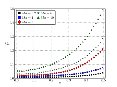
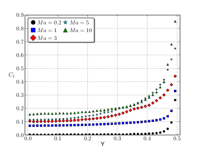
Figure 1: Half-channel profiles of $C_{0}$ and $C_{1}$ at $Kn=0.01$, for various $Ma$. The top ($Y=0.5$) and bottom ($Y=-0.5$) plates are moving with speeds $U_{w}$ in opposite directions.

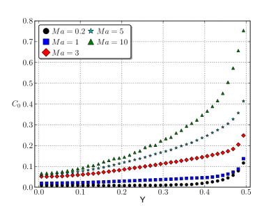
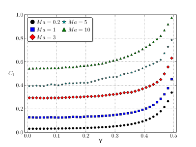
Figure 2: Half-channel profiles of $C_{0}$ and $C_{1}$ at $Kn=0.1$, for various $Ma$.The top ($Y=0.5$) and bottom ($Y=-0.5$) plates are moving with speeds $U_{w}$ in opposite directions.

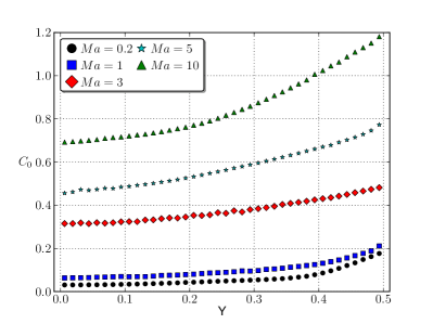
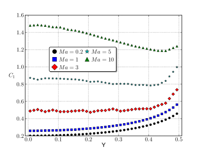
Figure 3: Half-channel profiles of $C_{0}$ and $C_{1}$ at $Kn=0.5$, for various $Ma$.

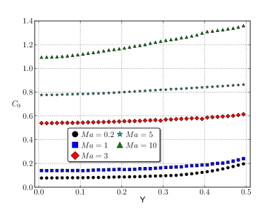
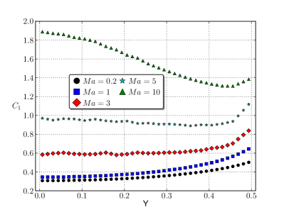
Figure 4: Half-channel profiles of $C_{0}$ and $C_{1}$ at $Kn=1$, for various $Ma$.The top ($Y=0.5$) and bottom ($Y=-0.5$) plates are moving with speeds $U_{w}$ in opposite directions.

The profiles of $C_{0}$ and $C_{1}$ for various Couette flow cases are presented in Figures 1-4. It is clearly shown that the level of non-equilibrium depends on both the Knudsen number and the Mach number ($Ma=U_{w}/\sqrt{RT_{0}}$). $C_{0}$, the indicator of departure from equilibrium, is small at $Kn=0.01$ especially in the bulk region ($Y$=0). However, when the Mach number increases, $C_{0}$ becomes larger. At a higher Mach number ($Ma=5$), the values of $C_{0}$ are even similar to those in a flow with a much higher Knudsen number (see $Kn=0.5$ and $Ma=0.2$ in Figure 3), showing that the extent of departure from equilibrium can be similar for two flows with very different Knudsen numbers. The Knudsen number alone does not determine the level of thermodynamic non-equilibrium.

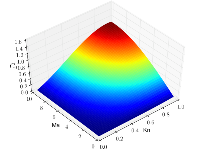
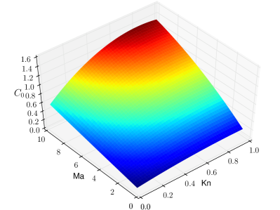
Figure 5: Dependence of $C_{0}$ on $Kn$ and $Ma$ in the bulk (left) and at the wall (right).

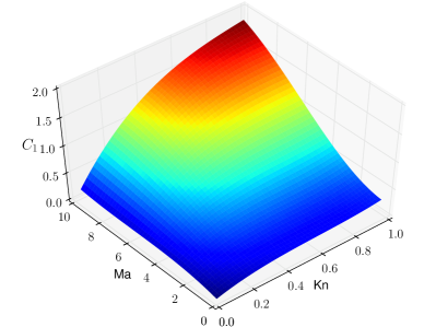
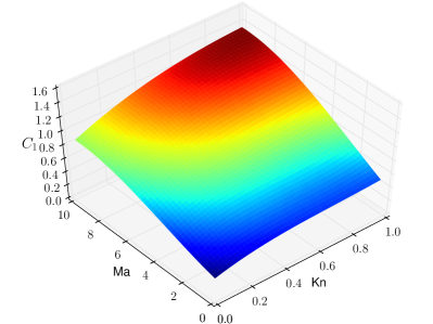
Figure 6: Dependence of $C_{1}$ on $Kn$ and $Ma$ in the bulk (left) and at the wall (right).

For a Knudsen number of $0.01$, the Navier-Stokes equations are usually regarded as valid. However, the value of $C_{1}$, which inversely indicates the appropriateness of using the Navier-Stokes equations, can increase with the Mach number, see Figure 1. When the Mach number is $1.0$ and above, a significant proportion of the non-equilibrium flow information cannot be captured by the Navier-Stokes equations, even in this simple flow configuration. When $Ma=0.2$, and in the bulk region ($Y=0$), the Navier-Stokes equations hold because $C_{1}\ll 1$. However, in the wall region, the Navier-Stokes equations are less accurate. The reason for this is the presence of Knudsen layer in the near-wall region, where the linear constitutive relation for stress that is assumed in the Navier-Stokes equations becomes inappropriate. When $Ma$ increases to $1.0$, higher-order fluid models may be required, even in the bulk, to accurately capture non-equilibrium information at conventional Knudsen numbers as low as 0.01.

For flows with $Kn$ around $0.1$, it is generally assumed that the Navier-Stokes equations will still be useful in the bulk flow region. Indeed, Figure 2 shows that less than $10\%$ error will be introduced to the non-equilibrium distribution function if the Navier-Stokes equations are used for a flow with $Ma=0.2$. However, $C_{1}$ is larger than $0.1$ in the bulk region when $Ma$ is above $0.2$, so substantial non-equilibrium flow information would not be captured by a Navier-Stokes analysis in these cases. Figure 3 also shows that non-equilibrium information cannot be properly captured, even for Mach numbers as low as $0.2$, when the Knudsen number becomes large (e.g. $0.5$). Figures 1-4 together show that neither the Knudsen number nor the simple product of Mach and Knudsen numbers can appropriately assess the level of thermodynamic non-equilibrium in flowfields. However, we can discover the appropriate dependencies of $C_{0}$ on $Kn$ and $Ma$ in certain flows.

When the Knudsen number is small, $f^{neq}\backsim f^{(1)}$ as a first order approximation, hence,

$$\begin{split}C_{0}&\sim\sqrt{\frac{\int(f^{(1)})^{2}d\bm{\xi}}{\int(f^{eq})^{2}d\bm{\xi}}}\\ &=\sqrt{\frac{\int(f^{eq})^{2}\left[\frac{\mu}{pRT}\frac{du<_{i}}{dx_{j>}}\varsigma_{<i}\varsigma_{j>}+\frac{2\kappa}{5pRT}\frac{dT}{dx_{i}}\varsigma_{i}\left(\frac{\varsigma_{j}\varsigma_{j}}{2RT}-\frac{5}{2}\right)\right]^{2}d\bm{\xi}}{\int(f^{eq})^{2}d\bm{\xi}}}.\end{split}$$ (10)

For Couette flows, this can be simplified to

$$C_{0}\sim\sqrt{\frac{\int(f^{eq})^{2}\left[\frac{\mu}{pRT}\frac{du{}_{x}}{dy}\varsigma_{x}\varsigma_{y}+\frac{2\kappa}{5pRT}\frac{dT}{dy}\varsigma_{y}\left(\frac{\varsigma_{x}^{2}+\varsigma_{y}^{2}+\varsigma_{z}^{2}}{2RT}-\frac{5}{2}\right)\right]^{2}d\bm{\xi}}{\int(f^{eq})^{2}d\bm{\xi}}}.$$ (11)

In the Navier-Stokes model, the velocity gradient turns out as $2U_{w}/{L}$ over the whole flowfield. The temperature gradient can vary with position, but is zero at the centerline and $\thicksim 2U_{w}^{2}\mu/\kappa L$ at the wall. So we estimate $C_{0}$ at the centerline from Eq.(11) to be

$$C_{0}\sim\frac{U_{w}\mu}{Lp}=\frac{\mu\sqrt{RT_{0}}}{pL}Ma\backsim KnMa,$$ (12)

and at the wall as

$$\begin{split}C_{0}&\sim\sqrt{\frac{7U_{w}^{4}\mu^{2}}{10L^{2}p^{2}RT}+\frac{U_{w}^{2}\mu^{2}}{L^{2}p^{2}}}\\ &\sim\sqrt{\frac{\mu^{2}RT_{0}}{p^{2}L^{2}}\frac{T_{0}}{T}Ma^{4}+\left(\frac{\mu\sqrt{RT_{0}}}{pL}Ma\right)^{2}}\\ &\sim KnMa\sqrt{1+Ma^{2}}.\end{split}$$ (13)

Therefore, the level of non-equilibrium increases with both the Knudsen and the Mach numbers. Note that this estimation is only appropriate when the Knudsen number is not too large. For large $Kn$, we need to analyse the relation numerically. For $C_{1}$, it is difficult to provide a solution even for small Knudsen numbers, as no generally agreed Burnett-order solution for $f^{(2)}$ is available. The numerical data shown in Figures 5 and 6 suggest a complicated general dependency of $C_{0}$ and $C_{1}$ on the Knudsen and Mach numbers.

In conclusion, we have addressed how to accurately assess the departure of flowfields from thermodynamic equilibrium, and how to identify when the Navier-Stokes model is applicable or not. Two new kinetic parameters based on the molecular velocity distribution function are proposed, with $C_{0}$ assessing how far flowfields are away from equilibrium, while $C_{1}$ indicating the validity of the Navier-Stokes model. Our MD numerical experiments conducted for Couette flows confirm that the flowfield and the appropriateness of the Navier-Stokes equations are not properly assessed by the Knudsen number alone, or even by the combination of Knudsen and Mach numbers proposed in the literature. The direct indicators $C_{0}$ and $C_{1}$ show a complicated dependency on both $Kn$ and $Ma$. Our proposed parameters are not only of theoretical interest, but could be used for model switching criteria in kinetic-continuum hybrid numerical schemes.

References

- Chapman and Cowling (1953) S. Chapman and T. G. Cowling, The Mathematical Theory of Non-Uniform Gases (Cambridge University Press, 1953), 3rd ed.
- Macrossan (2006) M. N. Macrossan, in Twenty-fifth Int. Symp. Rarefied Gas Dynamics, (2006), pp. 759–764.
- Tsien (1946) H. S. Tsien, J. Aerospace Sci. 13, 342 (1946).
- Wang and Boyd (2003) W.-L. Wang and I. D. Boyd, Phys. Fluids 15, 91 (2003).
- Lockerby et al. (2009) D. A. Lockerby, J. M. Reese, and H. Struchtrup, Proc. R. Soc. A 465, 1581 (2009).
- Garcia and Alder (1998) A. L. Garcia and B. J. Alder, J. Comput. Phys. 140, 66 (1998).
- Boyd et al. (1995) I. D. Boyd, G. Chen, and G. V. Candler, Phys. Fluids 7, 210 (1995).
- Hadjiconstantinou (2006) N. G. Hadjiconstantinou, Phys. Fluids 18, 111301 (2006).
- Yen (1984) S. M. Yen, Annu. Rev. Fluid Mech. 16, 67 (1984).
- Meng and Zhang (2011) J. Meng and Y. Zhang, J. Comput. Phys. 230, 835 (2011).
- Bird (1978) G. A. Bird, Annu. Rev. Fluid Mech. 10, 11 (1978).
- Macpherson and Reese (2008) G. B. Macpherson and J. M. Reese, Mol. Simul. 34, 97 (2008).
- Dongari et al. (2011) N. Dongari, Y. Zhang, and J. M. Reese, J. Phys. D: Appl. Phys. 44, 125502 (2011).