On uniqueness for time harmonic anisotropic Maxwell’s equations with piecewise regular coefficients

Abstract.

We are interested in the uniqueness of solutions to Maxwell’s equations when the magnetic permeability $\mu$ and the permittivity $\varepsilon$ are symmetric positive definite matrix-valued functions in $\mathbb{R}^{3}$. We show that a unique continuation result for globally $W^{1,\infty}$ coefficients in a smooth, bounded domain, allows one to prove that the solution is unique in the case of coefficients which are piecewise $W^{1,\infty}$ with respect to a suitable countable collection of sub-domains with $C^{0}$ boundaries. Such suitable collections include any bounded finite collection. The proof relies on a general argument, not specific to Maxwell’s equations. This result is then extended to the case when within these sub-domains the permeability and permittivity are only $L^{\infty}$ in sets of small measure.

1. Introduction

Suppose we are given a time-harmonic incident electric field $\mycal{E}^{i}$ and magnetic field $\mycal{H}^{i}$, special solutions of the time-harmonic homogeneous linear Maxwell equations of the form $\mycal{E}^{i}=\Re\left(\mathbf{E}^{i}e^{-i\omega t}\right)$ and magnetic field $\mycal{H}^{i}=\Re\left(\mathbf{H}^{i}e^{-i\omega t}\right)$, where $\mathbf{E}^{i}\in H_{\textrm{loc}}^{1}\left(\mathbb{R}^{3}\right)^{3}$ and $\mathbf{H}^{i}\in H_{\textrm{loc}}^{1}\left(\mathbb{R}^{3}\right)^{3}$ are complex-valued solutions of the homogeneous time-harmonic Maxwell equations

$$\nabla\wedge\mathbf{E}^{i}-i\,\omega\mu_{0}\mathbf{H}^{i} =0\textrm{ in }\mathbb{R}^{3},$$

$$\nabla\wedge\mathbf{H}^{i}+i\,\omega\varepsilon_{0}\mathbf{E}^{i} =0\textrm{ in }\mathbb{R}^{3},$$

where $\mu_{0}$ and $\varepsilon_{0}$ are positive constants, representing respectively the magnetic permeability and the electric permittivity of vacuum, and $\omega\in\mathbb{R}\setminus\{0\}$. The full time-harmonic electromagnetic field $(\mathbf{E},\mathbf{H})\in H_{\textrm{loc}}\left(\textrm{curl};\mathbb{R}^{3}\right)$, where for any domain $W$ we define

$$H_{\textrm{loc}}\left(\textrm{curl};W\right):=\left\{\mathbf{u}\in L_{\textrm{loc}}^{2}\left(W\right)^{3}\textrm{ such that }\nabla\wedge\mathbf{u}\in L_{\textrm{loc}}^{2}\left(W\right)^{3}\right\},$$

satisfies Maxwell’s equations

(1.1) $$\nabla\wedge\mathbf{E}-i\,\omega\mu_{0}\mu(x)\,\mathbf{H} =0\textrm{ in }\mathbb{R}^{3},$$

$$\nabla\wedge\mathbf{H}+i\,\omega\varepsilon_{0}\varepsilon(x)\,\mathbf{E} =0\textrm{ in }\mathbb{R}^{3},$$

where $\varepsilon$ and $\mu$ are real matrix-valued functions in $L^{\infty}\left(\mathbb{R}^{3}\right)^{3\times 3}$. Decomposing the full electromagnetic field into its incident part and its scattered part,

(1.2) $$\mathbf{E}^{s}:=\mathbf{E}-\mathbf{E}^{i},\textrm{ and }\mathbf{H}^{s}:=\mathbf{H}-\mathbf{H}^{i},$$

we assume that the scattered field satisfies the Silver-Müller radiation condition, uniformly in all directions, that is, if $x:=r\theta$ then

(1.3) $$\lim_{r\to\infty}\sup_{\theta\in S^{2}}\left|\mathbf{H}^{s}\left(r\theta\right)\wedge r\theta-r\mathbf{\mathbf{E}}^{s}\left(r\theta\right)\right|=0,$$

where $S^{2}:=\{x\in\mathbb{R}^{3}\textrm{ such that }|x|=1\}$ denotes the unit sphere.

This paper is about the existence of a unique solution to (1.1) satisfying (1.2) and (1.3), under the following additional hypotheses on $\varepsilon$ and $\mu$. We assume that both permittivity and permeability are real symmetric, uniformly positive definite and bounded, that is, there exist $0<\alpha\leq\beta<\infty$ such that for all $\xi\in\mathbb{R}^{3}$ and almost every $x\in\mathbb{R}^{3}$,

(1.4) $$\alpha\left|\xi\right|^{2} \leq\varepsilon(x)\xi\cdot\xi\leq\beta\left|\xi\right|^{2},$$

(1.5) $$\alpha\left|\xi\right|^{2} \leq\mu(x)\xi\cdot\xi\leq\beta\left|\xi\right|^{2}.$$

We suppose that $\varepsilon$ and $\mu$ vary only in an open bounded domain $\Omega$, so that

(1.6) $$\varepsilon=\mu=\mathbf{I}_{3}\textrm{ in }{\Omega}^{c}=\mathbb{R}^{3}\setminus{\Omega},$$

where $\mathbf{I}_{3}$ is the identity matrix in $\mathbb{R}^{3\times 3}$. We assume that $\Omega$ is of the form

(1.7) $$\Omega=\textrm{int}\left({\underset{i\in I}{\cup}}\bar{\Omega}_{i}\right),$$

where the sub-domains $\Omega_{i}$, $i\in I\subset\mathbb{N}$ are disjoint and of class $C^{0}$, and int denotes the interior. The permittivity $\varepsilon$ and the permeability $\mu$ are assumed to be piecewise $W^{1,\infty}$ with respect to the sub-domains $\Omega_{i}$, so that for each $i\in I$, there exist $\varepsilon_{i},\mu_{i}\in W^{1,\infty}\left(\mathbb{R}^{3}\right)^{3\times 3}$ satisfying (1.4)-(1.5) and

(1.8) $$\|\varepsilon_{i}\|_{W^{1,\infty}(\mathbb{R}^{3})^{3\times 3}}+\|\mu_{i}\|_{W^{1,\infty}(\mathbb{R}^{3})^{3\times 3}}\leq M_{i},$$

where $M_{i}>0$ is a positive constant, such that

(1.9) $$\varepsilon(x)=\varepsilon_{i}(x)\textrm{ and }\mu(x)=\mu_{i}(x),\quad\textrm{a.e. }x\in\Omega_{i}\,.$$

Given a bounded set $A\subset\mathbb{R}^{3}$, we write $\mathcal{U}\left(A\right)$ as the (unique) unbounded component of $\bar{A}^{c}$.

Assumption 1.

For any $J\subset I$, and $\Omega_{J}=\textrm{\rm int}\left({\underset{j\in J}{\cup}}\bar{\Omega}_{j}\right)$, there exists $j_{0}\in J$ such that $\partial\mathcal{U}\left(\Omega_{J}\right)\cap\partial\Omega_{j_{0}}$ admits an interior point relative to $\partial\mathcal{U}\left(\Omega_{J}\right)$. In other words, there exist $j_{0}\in J$ and $x_{0}\in\partial\mathcal{U}\left(\Omega_{J}\right)\cap\partial\Omega_{j_{0}}$ such that $B(x_{0},\delta)\cap\partial\mathcal{U}\left(\Omega_{J}\right)\subset\partial\Omega_{j_{0}}$ for some $\delta>0$.

Proposition 1.

Assumption 1 holds if for all $J\subset I$, there exist $x_{J}\in\partial\mathcal{U}\left(\Omega_{J}\right)$ and $\delta_{J}>0$ such that $B(x_{J},\delta_{J})\cap\Omega_{j}\neq\emptyset$ for only finitely many $j\in J$. In particular, Assumption 1 holds when $I$ is finite.

Proof.

Given $J$, $x_{J}\in\partial\mathcal{U}\left(\Omega_{J}\right)$ and $\delta_{J}$ as in the statement of the proposition let $B_{J}=B(x_{J},\delta_{J})$ and let $J^{\prime}$ be the finite subset of $J$ such that $B_{J}\cap\underset{j\in J}{\cup}\Omega_{j}=B_{J}\cap\underset{j\in J^{\prime}}{\cup}\Omega_{j}$. We first show that

(1.10) $$\partial\mathcal{U}\left(\Omega_{J}\right)\cap B_{J}=\underset{j\in J}{\cup}\left(\partial\mathcal{U}\left(\Omega_{J}\right)\cap B_{J}\right)\cap\partial{\Omega}_{j}.$$

Indeed, let $x\in\partial\mathcal{U}\left(\Omega_{J}\right)\cap B_{J}$. Then $x\not\in\underset{j\in J}{\cup}\Omega_{j}$. We claim that there exists a sequence $x_{k}\in{\underset{j\in J}{\cup}}{\Omega}_{j}$ such that $x_{k}$ tends to $x$. If not, for some $\eta>0$ sufficiently small, we would have $B(x,\eta)\subset B_{J}$ , and $B(x,\eta)\cap{\underset{j\in J}{\cup}}{\Omega}_{j}=B(x,\eta)\cap{\underset{j\in J^{\prime}}{\cup}}{\Omega}_{j}=\emptyset$. On the other hand, there exists a sequence $y_{k}\in\mathcal{U}\left(\Omega_{J}\right)$ such that $y_{k}$ tends to $x$. But $B(x,\eta)$ is connected and contained in $\bar{\Omega}_{J}^{c}$, thus $B(x,\eta)\subset\mathcal{U}\left(\Omega_{J}\right)$. This contradiction proves the claim.

Next, we note that $\partial\mathcal{U}\left(\Omega_{J}\right)$ is closed, thus complete in the subspace topology induced by $\mathbb{R}^{3}$. Its intersection with the open ball $B_{J}$ is an open subspace of $\partial\mathcal{U}\left(\Omega_{J}\right)$ by definition of the subspace topology. It is therefore a Baire space (see e.g. [11]). If a Baire Space is a countable union of closed sets, then one of the sets has an interior point. Using the identity (1.10), we obtain that there exists $j_{0}$ such that $\partial\mathcal{U}\left(\Omega_{J}\right)\cap B_{J}\cap\partial\Omega_{j_{0}}$ admits an interior point relative to $\partial\mathcal{U}\left(\Omega_{J}\right)\cap B_{J}$, that is, there exist $j_{0}\in J$, $x_{0}\in\partial\mathcal{U}\left(\Omega_{J}\right)\cap B_{J}$ and $\delta>0$ such that $B(x_{0},\delta)\cap\partial\mathcal{U}\left(\Omega_{J}\right)\cap B_{J}\subset\partial\Omega_{j_{0}}$.

Since $B_{J}$ is open, $B(x_{0},\delta)\cap B_{J}=B(x_{0},\delta)$ when $\delta$ is sufficiently small, and we have established that Assumption 1 holds. ∎

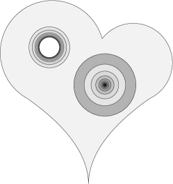
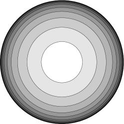
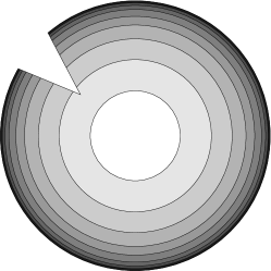
Figure 1. Left: an infinite collection of sub-domains satisfying Assumption 1. Centre: an infinite collection of sub-domains excluded by Assumption 1. Right: this collection satisfies Assumption 1.

An example of a collection of sub-domains excluded by Assumption 1 is a collection of concentric shells concentrating on an exterior boundary, such as

(1.11) $$\Omega_{i}=B\left(\mathbf{0},\frac{i}{i+1}\right)\setminus\bar{B}\left(\mathbf{0},\frac{i-1}{i}\right),\quad i=1,2,3,\ldots$$

In such a case, $\partial\mathcal{U}\left(\Omega\right)$ is the unit sphere, which is not the boundary of any of the subsets. On the other hand, Assumption 1 allows the sub-domains $\Omega_{i}$ to concentrate at a point or near an interior boundary. In Figure 1, we represent on the left a non-Lipschitz non-simply connected domain $\Omega$ which satisfies Assumption 1. In the centre, the domain given by (1.11) excluded by Assumption 1 is shown. On the right, we sketch a domain inspired by the one described by (1.11) which satisfies Assumption 1: near the accumulating boundary, interior points can be found on the wedge-shaped slit in the domain.

2. Main result

Our main result is the following theorem.

Theorem 2.

Assume that (1.4)–(1.9) and Assumption 1 hold. If for a given $\omega\neq 0$, $\mathbf{E}\in H_{\rm{loc}}\left(\rm{curl};\mathbb{R}^{3}\right)$ and $\mathbf{H}\in H_{\rm{loc}}\left(\rm{curl};\mathbb{R}^{3}\right)$ are solutions of (1.1)–(1.3) corresponding to $\mathbf{E}^{i}=0$ and $\mathbf{H}^{i}=0$, then $\mathbf{E}=\mathbf{H}=0$.

There is a very long history concerning this problem, under various assumptions on the coefficients, see e.g. [1, 2, 3, 6, 7, 10, 13, 12, 14, 16] and the references therein. The improvement provided by the result in this work is that we assume that $\varepsilon$, $\mu$ are matrix-valued functions and that the sub-domains $\Omega_{i}$ are only of class $C^{0}$. We do not assume that the sub-domains are Lipschitz as assumed for example in [6] for the isotropic (scalar) case. The authors are not aware of the existence of a general uniqueness result for the above problem when the coefficients are just $C^{0,\alpha}$ Hölder continuous, with $\alpha<1$. For general elliptic equations, counter-examples to unique continuation, the main technique for proving uniqueness, are known in that case, see [8]. We remind the reader of the definition of a domain of class $C^{0}$.

Definition 3.

A bounded domain $\Omega$ of $\mathbb{R}^{3}$ is of class $C^{0}$ if for any point $x_{0}$ on the boundary $\partial\Omega$, there exists a ball $B\left(x_{0},\delta\right)$ and an orthogonal coordinate system $(x_{1},x_{2},x_{3})$ with origin at $x_{0}$ such that there exists a continuous function $f:\,C^{0}\left(\mathbb{R}^{2};\mathbb{R}\right)$ that satisfies

$$\Omega\cap B\left(x_{0},\delta\right)=\left\{x\in B\left(x_{0},\delta\right):x_{3}>f\left(x_{1},x_{2}\right)\right\}.$$

We define $B_{0}$ as the smallest open ball containing $\Omega$. Note that the uniqueness of the solution outside $B_{0}$ is well known, due to the so-called Rellich’s Lemma, see e.g. [2].

Lemma 4 (Rellich’s Lemma).

If for a fixed $\omega$, $\mathbf{E}\in H_{{\rm{loc}}}\left({\rm{curl}};\mathbb{R}^{3}\right)$ and $\mathbf{H}\in H_{{\rm{loc}}}\left({\rm{curl}};\mathbb{R}^{3}\right)$ are solutions of (1.1)-(1.3) corresponding to $\mathbf{E}^{i}=0$ and $\mathbf{H}^{i}=0$, then $\mathbf{E}=\mathbf{H}=0$ in $\bar{B}_{0}^{c}$.

Our proof relies on a recent unique continuation result [13] proved for globally $W^{1,\infty}$ regular coefficients.

Theorem 5 ([13]).

Let $V$ be a connected open set in $\mathbb{R}^{3}$. Assume that $\varepsilon$ and $\mu$ are two real symmetric matrix valued functions in $V$ satisfying (1.4)–(1.5), and

$$\|\varepsilon\|_{W^{1,\infty}(V)^{3\times 3}}+\|\mu\|_{W^{1,\infty}(V)^{3\times 3}}\leq M,$$

for some constant $M>0$. Suppose $(\mathbf{E},\mathbf{H})\in\left(L^{2}_{\rm{loc}}\left(V\right)\right)^{2}$ satisfy

$$\nabla\wedge\mathbf{E}-i\,\omega\mu_{0}\mu(x)\,\mathbf{H} =0\textrm{ in }V,$$

$$\nabla\wedge\mathbf{H}+i\,\omega\varepsilon_{0}\varepsilon(x)\,\mathbf{E} =0\textrm{ in }V.$$

Then, there exist $s>0$ independent of $V$, $\mathbf{E}$ and $\mathbf{H}$, such that if for some $x_{0}\in V$, and for all $N\in\mathbb{N}$ and all $\delta>0$ sufficiently small,

$$\int_{B(x_{0},\delta)}\left(\left|\mathbf{E}\right|^{2}+\left|\mathbf{H}\right|^{2}\right)dx\leq C_{N}\exp\left(-N\delta^{-s}\right)$$

for some constant $C_{N}>0$, then $\mathbf{E}=\mathbf{H}=0$ in $V$.

The proof of Theorem 2 consists of three steps. The first two steps are given by the two propositions below.

Proposition 6.

Under the hypothesis of Theorem 2, suppose that $A\subset\mathbb{R}^{3}$ is a bounded open set and that for almost every $x\in\mathcal{U}\left(A\right)$ either $\varepsilon(x)=\mu(x)=\mathbf{I}_{3}$ or $\mathbf{E}(x)=\mathbf{H}(x)=0$. Then $\mathbf{E}=\mathbf{H}=0$ in $\mathcal{U}\left(A\right)$.

Proof.

For any $\mathbf{v,w}\in L^{2}\left(\mathcal{U}\left(A\right)\right)^{2}$, we have

(2.1) $$\int_{\mathcal{U}\left(A\right)}\nabla\wedge\mathbf{E}\cdot\mathbf{v}\,dx-i\omega\mu_{0}\int_{\mathcal{U}\left(A\right)}\mu(x)\mathbf{H}\cdot\mathbf{v}\,dx =0,$$

(2.2) $$\int_{\mathcal{U}\left(A\right)}\nabla\wedge\mathbf{H}\cdot\mathbf{w}\,dx+i\omega\varepsilon_{0}\int_{\mathcal{U}\left(A\right)}\epsilon(x)\mathbf{E}\cdot\mathbf{w}\,dx =0,$$

where the integrals (2.1) and (2.2) are well defined by Rellich’s Lemma 4. Since for almost every $x$ in $\mathcal{U}\left(A\right)$, either $\varepsilon(x)=\mu(x)=\mathbf{I}_{3}$ or $\mathbf{E}=\mathbf{H}=0$, the solutions of the system (2.1)-(2.2) can be written also in the form

$$\int_{\mathcal{U}\left(A\right)}\nabla\wedge\mathbf{E}\cdot\mathbf{v}\,dx-i\omega\mu_{0}\int_{\mathcal{U}\left(A\right)}\mathbf{H}\cdot\mathbf{v}\,dx =0,$$

$$\int_{\mathcal{U}\left(A\right)}\nabla\wedge\mathbf{H}\cdot\mathbf{w}\,dx+i\omega\varepsilon_{0}\int_{\mathcal{U}\left(A\right)}\mathbf{E}\cdot\mathbf{w}\,dx =0,$$

which is the weak formulation of

$$\nabla\wedge\mathbf{E}-i\,\omega\mu_{0}\,\mathbf{H} =0\textrm{ in }\mathcal{U}\left(A\right),$$

$$\nabla\wedge\mathbf{H}+i\,\omega\varepsilon_{0}\,\mathbf{E} =0\textrm{ in }\mathcal{U}\left(A\right).$$

Next, since $A$ is bounded, thanks to Rellich’s Lemma 4, $\mathbf{E}=\mathbf{H}=0$ in $\mathcal{U}\left(A\right)\cap\left(\mathbb{R}^{3}\setminus\bar{B}(R)\right)$, for $R$ large enough. In particular, $\mathbf{E}$ and $\mathbf{H}$ vanish in a ball contained in $\mathcal{U}\left(A\right)$, which is open and connected, and the conclusion follows from Theorem 5, applied with $\varepsilon(x)=\mu(x)=\mathbf{I}_{3}$, which in this case reduces to a well known result concerning the Helmholtz equation. ∎

Proposition 7.

Let

$$J:=\{i\in I:\left|\mathbf{E}(x)\right|^{2}+\left|\mathbf{H}(x)\right|^{2}>0\textrm{ on a set of positive measure in }\Omega_{i}\}.$$

Then $J=\emptyset$.

Proof.

Suppose for contradiction that $J$ is nonempty. Then, by Assumption 1 there exists $x_{0}\in\partial\mathcal{U}\left(\Omega_{J}\right)\cap\partial\Omega_{j_{0}}$ such that $B(x_{0},\delta)\cap\partial\mathcal{U}\left(\Omega_{J}\right)\subset\partial\Omega_{j_{0}}$ for some $j_{0}\in J$ and $\delta>0$. To simplify notation, set $j_{0}=1$.

Let us show that there exist a point $c$ on $\partial\mathcal{U}\left(\Omega_{J}\right)\cap\partial\Omega_{1}$ and a radius $\tilde{\delta}>0$ such that

(2.3) $$\Omega_{J}\cap B(c,\tilde{\delta})=\Omega_{1}\cap B(c,\tilde{\delta}).$$

Figure 2 sketches the configuration we have at hand around $c$.

Figure 2. A ball centred at an interior point on the boundary of $\mathcal{U}\left(\Omega_{J}\right)$.

Since $\Omega_{1}$ has a $C^{0}$ boundary, for some (smaller) $\delta>0$ there exists a continuous map $f$ and a suitable orientation of axes such that $B(x_{0},\delta)\cap\partial\Omega_{J}\subset\partial\Omega_{1}$ and

$$\Omega_{1}\cap B(x_{0},\delta)=\left\{x\in B\left(x_{0},\delta\right):x_{3}>f\left(x_{1},x_{2}\right)\right\}.$$

This alone does not prove our claim, since $B(x_{0},\delta)$ could still intersect $\Omega_{J}$ when $x_{3}\leq f(x_{1},x_{2})$. Since $x_{0}\in\partial\mathcal{U}\left(\Omega_{J}\right)$, there exists a sequence $\left\{y_{j}\right\}\subset\mathcal{U}\left(\Omega_{J}\right)\cap B(x_{0},\delta)$ such that $y_{j}$ tends to $x_{0}$. Consider for a fixed and sufficiently large $j$ the line segment $\{y_{j}+te_{3},t\geq 0\}$, and let $\tau>0$ be the least value of $t$ such that $y_{j}+te_{3}\in\partial\Omega_{J}$. Then, $y_{j}+te_{3}\not\in\bar{\Omega}_{J},$ for $t<\tau$, and $y_{j}+\tau e_{3}\in\partial\Omega_{1}$. Hence $y_{j}+\tau e_{3}\not\in\underset{k\in J,k>1}{\cup}\Omega_{k}$. Since the sets $\Omega_{k}$ are disjoint, the line segment does not intersect $\underset{k\in J,k>1}{\cup}\Omega_{k}$ in $B(x_{0},\delta)$. The same argument applies to any line segment $\{z+te_{3},t\geq 0\}$ for $z$ sufficiently close to $y_{j}$. Introducing $c=y_{j}+\tau e_{3}$ we have established that there exists a ball $B\left(c,\tilde{\delta}\right)$ such that $\Omega_{1}\cap B\left(c,\tilde{\delta}\right)=\Omega_{J}\cap B\left(c,\tilde{\delta}\right)$, which is (2.3).

Now, thanks to Proposition 6, and noting that (by Fubini’s Theorem) each $\partial\Omega_{i}$ is of measure zero, $\mathbf{E}=\mathbf{H}=0$ almost everywhere in $\mathcal{U}\left(\Omega_{J}\right)$. Thus, for almost every $x\in B(c,\tilde{\delta})$, either $\mathbf{E}=\mathbf{H}=0$ or $\varepsilon(x)=\varepsilon_{1}(x)$, and $\mu(x)=\mu_{1}(x)$. Considering the weak formulation of Maxwell’s equations, and arguing as in the proof of Proposition 6, we note that $\mathbf{E}$ and $\mathbf{H}$ are weak solutions of

$$\nabla\wedge\mathbf{E}-i\,\omega\mu_{0}\mu_{1}(x)\,\mathbf{H} =0\textrm{ in }B(c,\tilde{\delta}),$$

$$\nabla\wedge\mathbf{H}+i\,\omega\varepsilon_{0}\varepsilon_{1}(x)\,\mathbf{E} =0\textrm{ in }B(c,\tilde{\delta}),$$

and vanish on the connected non-empty open set $B(c,\tilde{\delta})\cap\{x_{3}<f(x_{1},x_{2})\}$. Since $\epsilon_{1}$ and $\mu_{1}$ satisfy (1.8), that is,

$$\|\varepsilon_{1}\|_{W^{1,\infty}(\mathbb{R}^{3})^{3\times 3}}+\|\mu_{1}\|_{W^{1,\infty}(\mathbb{R}^{3})^{3\times 3}}\leq M_{1},$$

Theorem 5 shows that $\mathbf{E}=\mathbf{H}=0$ in $B(c,\tilde{\delta})$. This in turn shows that $\mathbf{E}$ and $\mathbf{H}$ vanish on a ball inside $\Omega_{1}$, and applying Theorem 5 in $\Omega_{1}$ we obtain $\mathbf{E}=\mathbf{H}=0$ almost everywhere in $\Omega_{1}$. This contradiction concludes the proof. ∎

We now turn to the final step. We have obtained that $\mathbf{E}=\mathbf{H}=0$ almost everywhere in $\Omega$, and therefore either $\mathbf{E}=\mathbf{H}=0$ or $\varepsilon(x)=\mu(x)=\mathbf{I}_{3}$ almost everywhere in $\mathbb{R}^{3}$. Arguing as above, we deduce that $(\mathbf{E},\mathbf{H})$ is a weak solution of (1.1) with $\varepsilon(x)=\mu(x)=\mathbf{I}_{3}$ everywhere and the conclusion of Theorem 2 follows from Rellich’s Lemma.

3. The case of a medium with defects

We extend our result to the case when defects of small measure are allowed in the medium. One application is to liquid crystals (see [15] for more details). Namely, we assume that the permittivity and permeability are of the form

(3.1) $$\varepsilon_{D} =\left(1-\mathbf{1}_{D}\right)\varepsilon+\mathbf{1}_{D}\tilde{\varepsilon},$$

$$\mu_{D} =\left(1-\mathbf{1}_{D}\right)\mu+\mathbf{1}_{D}\tilde{\mu},$$

where $\varepsilon$ and $\mu$ satisfy (1.4)-(1.9), $\mathbf{1}_{D}$ is the indicator function of a measurable bounded set $D$, such that

(3.2) $$D\subset{\underset{i\in I}{\cup}}\Omega_{i},\quad\overline{D\cap\Omega_{i}}\subset\Omega_{i}\mbox{ and }\Omega_{i}\setminus\overline{D\cap\Omega_{i}}\textrm{ is connected for each }i\in I,$$

and $\tilde{\epsilon}$ and $\tilde{\mu}$ are real symmetric positive definite matrices in $L^{\infty}\left(\mathbb{R}^{3}\right)^{3\times 3}$ satisfying (1.4)-(1.5).

Theorem 8.

Suppose that the electric and magnetic fields $\mathbf{E}_{D}\in H_{\textrm{\rm loc}}\left(\textrm{\rm curl};\mathbb{R}^{3}\right)$ and $\mathbf{H}_{D}\in H_{\textrm{\rm loc}}\left(\textrm{\rm curl};\mathbb{R}^{3}\right)$ are solutions of

(3.3) $$\nabla\wedge\mathbf{E}_{D}-i\,\omega\mu_{0}\mu_{D}(x)\,\mathbf{H}_{D} =0\textrm{ in }\mathbb{R}^{3},$$

$$\nabla\wedge\mathbf{H}_{D}+i\omega\varepsilon_{0}\varepsilon_{D}(x)\,\mathbf{E}_{D} =0\textrm{ in }\mathbb{R}^{3},$$

together with the Silver-Müller radiation condition (1.3), and that $\varepsilon_{D}$ and $\mu_{D}$ are given by (3.1), with $D$ satisfying (3.2). Suppose Assumption 1 holds. Then, there exists a constant $d_{0}>0$ depending only on the measure $|B_{0}|$ of $B_{0}$, $|\omega|$ and the lower and upper bounds $\alpha$ and $\beta$ given in (1.4)-(1.5) such that if the measure of $D$ satisfies $\left|D\right|<d_{0}$, then $\mathbf{E}_{D}=\mathbf{H}_{D}=0$ almost everywhere.

To prove Theorem 8, we use the following variant of Theorem 2.

Proposition 9.

Under the same assumptions as Theorem 2, and assuming that (3.2) holds,

$${\rm supp}\,\mathbf{H}_{D}\cup{\rm supp}\,\mathbf{E}_{D}\subset\bar{D}.$$

Proof.

The proof follows from that of Theorem 2, since by assumption for each $i\in I$, $\overline{D\cap\Omega_{i}}\subset\Omega_{i}$, and the boundary of $\Omega\setminus\Omega_{i}$ is unaltered by the defects. ∎

Proof of Theorem 8.

Since (3.3) admits a weak formulation, arguing as before we see using Proposition 9 that $\mathbf{E}_{D}\in H\left(\textrm{curl};B_{0}\right)$ and $\mathbf{H}_{D}\in H\left(\textrm{curl};B_{0}\right)$ have compact support in $B_{0}$ and are also solutions of

$$\nabla\wedge\mathbf{E}_{D}-i\omega\mu_{0}\hat{\mu}\,\mathbf{H}_{D} =0\textrm{ in }B_{0},$$

$$\nabla\wedge\mathbf{H}_{D}+i\omega\varepsilon_{0}\hat{\epsilon}\,\mathbf{E}_{D} =0\textrm{ in }B_{0},$$

where $\hat{\varepsilon}=\mathbf{I}_{3}+\mathbf{1}_{D}\left(\tilde{\varepsilon}-\mathbf{I}_{3}\right),$ and $\hat{\mu}=\mathbf{I}_{3}+\mathbf{1}_{D}\left(\tilde{\mu}-\mathbf{I}_{3}\right)$. Note that $i\omega\mu_{0}\hat{\mu}\,\mathbf{H}_{D}$ has compact support and is divergence free. Thus the Helmholtz decomposition (see e.g. [4, 5, 9]) of $i\omega\mu_{0}\hat{\mu}\,\mathbf{H}_{D}$ shows there exists a unique $\mathbf{A}_{H}\in H^{1}\left(B_{0}\right)^{3}$ such that $\mathbf{A}_{H}\cdot\nu=0,$ on $\partial B_{0}$, $\textrm{div}\left(\mathbf{A}_{H}\right)=0$ and such that $i\omega\mu_{0}\hat{\mu}\,\mathbf{H}_{D}=\nabla\wedge\mathbf{A}_{H}$. Furthermore, $\mathbf{A}_{H}$ satisfies

$$\left\|\nabla\mathbf{A}_{H}\right\|_{L^{2}\left(B_{0}\right)^{3\times 3}} \leq C\left(\left\|\nabla\wedge\mathbf{A}_{H}\right\|_{L^{2}\left(B_{0}\right)^{3}}+\left\|\mathbf{A}_{H}\right\|_{L^{2}\left(B_{0}\right)^{3}}\right)$$

$$\mbox{ and }\left\|\mathbf{A}_{H}\right\|_{L^{2}\left(B_{0}\right)^{3}} \leq C|B_{0}|^{1/3}\left\|\nabla\wedge\mathbf{A}_{H}\right\|_{L^{2}\left(B_{0}\right)^{3}},$$

where $C$ is a universal constant. Altogether this yields

(3.4) $$\left\|\nabla\mathbf{A}_{H}\right\|_{L^{2}\left(B_{0}\right)^{3\times 3}}\leq C\beta\mu_{0}|\omega|\left(\left|B_{0}\right|+1\right)^{1/3}\left\|\mathbf{H}_{D}\right\|_{L^{2}\left(B_{0}\right)^{3}}.$$

Since $\mathbf{E}_{D}-\mathbf{A}_{H}$ is curl free, we deduce that there exists $p\in H^{1}\left(B_{0}\right)$ such that $\mathbf{E}_{D}=\mathbf{A}_{H}+\nabla p$, and $p$ is uniquely defined by setting $\int_{B_{0}}p\,dx=0$. Noticing that $\hat{\varepsilon}\mathbf{E}_{D}$ is divergence free, and $\hat{\varepsilon}-\mathbf{I}_{3}$ is compactly supported in $B_{0}$ we have that $p$ is the solution of

$$\textrm{div}\left(\hat{\varepsilon}\nabla p\right) =-\textrm{div}\left(\hat{\varepsilon}\mathbf{A}_{H}\right)\textrm{ in }B_{0},$$

$$\nabla p\cdot n =0\textrm{ on }\partial B_{0},$$

$$\int_{B_{0}}p\,dx =0.$$

Since $\mathbf{A}_{H}$ is divergence free, the right-hand side becomes

$$-\textrm{div}\left(\hat{\varepsilon}\mathbf{A}_{H}\right)=-\textrm{div}\left(\mathbf{1}_{D}\left(\tilde{\varepsilon}-\mathbf{I}_{3}\right)\mathbf{A}_{H}\right).$$

To proceed, we compute using the Cauchy-Schwarz inequality the following bound

$$\alpha\left\|\nabla p\right\|^{2}_{L^{2}(B_{0})^{3}}\leq\int_{B_{0}}\hat{\epsilon}\nabla p\cdot\nabla p\,dx =-\int_{B_{0}}\mathbf{1}_{D}\left(\tilde{\varepsilon}-\mathbf{I}_{3}\right)\mathbf{A}_{H}\cdot\nabla p\,dx$$

$$\leq\left(\beta+1\right)\left\|\mathbf{A}_{H}\right\|_{L^{2}(D)^{3}}\left\|\nabla p\right\|_{L^{2}(B_{0})^{3}},$$

and we have obtained that

$$\left\|\nabla p\right\|_{L^{2}(B_{0})^{3}}\leq\frac{\beta+1}{\alpha}\left\|\mathbf{A}_{H}\right\|_{L^{2}(D)^{3}}.$$

Next note using Proposition 9 that

$$\left\|\mathbf{E}_{D}\right\|_{L^{2}\left(B_{0}\right)^{3}}=\left\|\mathbf{E}_{D}\right\|_{L^{2}\left(D\right)^{3}}\leq\left\|\nabla p\right\|_{L^{2}\left(B_{0}\right)^{3}}+\left\|\mathbf{A}_{H}\right\|_{L^{2}\left(D\right)^{3}}\leq\frac{2\beta+1}{\alpha}\left\|\mathbf{A}_{H}\right\|_{L^{2}\left(D\right)^{3}}.$$

The Sobolev-Gagliardo-Nirenberg inequality in $B_{0}$ shows that

$$\left\|\mathbf{A}_{H}\right\|_{L^{6}\left(B_{0}\right)^{3}}\leq C\left(\left|B_{0}\right|+1\right)^{1/3}\left\|\mathbf{A}_{H}\right\|_{H^{1}\left(B_{0}\right)^{3}},$$

where $C$ is a universal constant. Therefore, using Hölder’s inequality, together with the Poincaré-Friedrichs estimate (3.4), we have

$$\left\|\mathbf{A}_{H}\right\|_{L^{2}\left(D\right)^{3}}\leq\left|D\right|^{\frac{1}{3}}\left\|\mathbf{A}_{H}\right\|_{L^{6}\left(B_{0}\right)^{3}}\leq C\beta\left(\left|B_{0}\right|+1\right)^{2/3}\mu_{0}|\omega|\left|D\right|^{\frac{1}{3}}\left\|\mathbf{H}_{D}\right\|_{L^{2}\left(B_{0}\right)^{3}}.$$

Altogether we have obtained

(3.5) $$\left\|\mathbf{E}_{D}\right\|_{L^{2}\left(B_{0}\right)^{3}}\leq C\frac{\beta(\beta+1)}{\alpha}\left(\left|B_{0}\right|+1\right)^{2/3}\mu_{0}|\omega|\left|D\right|^{\frac{1}{3}}\left\|\mathbf{H}_{D}\right\|_{L^{2}\left(B_{0}\right)^{3}}.$$

Repeating the same argument, but starting with $\mathbf{H}_{D}$, we obtain also

(3.6) $$\left\|\mathbf{H}_{D}\right\|_{L^{2}\left(B_{0}\right)^{3}}\leq C\frac{\beta(\beta+1)}{\alpha}\left(\left|B_{0}\right|+1\right)^{2/3}\varepsilon_{0}|\omega|\left|D\right|^{\frac{1}{3}}\left\|\mathbf{E}_{D}\right\|_{L^{2}\left(B_{0}\right)^{3}}.$$

The inequalities (3.5) and (3.6) imply that $\mathbf{H}_{D}=\mathbf{E}_{D}=0$ when

(3.7) $$\left|D\right|<d_{0}:=C\frac{\alpha^{3}}{\beta^{3}(\beta+1)^{3}(\left|B_{0}\right|+1)^{2}\left(\sqrt{\varepsilon_{0}\mu_{0}}|\omega|\right)^{3}}\,,$$

where $C$ is a universal constant. ∎

Remark 10.

The dependence of the threshold constant $d_{0}$ given by (3.7) on $|\omega|$ and $\left|B_{0}\right|$ shows that for a permeability $\mu$ and a permittivity $\varepsilon$ satisfying (1.4), (1.5) and (1.6) only, uniqueness for Maxwell’s equations holds provided, if $\omega$ is fixed, the domain $\Omega$ is of small measure and bounded diameter, or, for a given $\Omega$, when the absolute value of the frequency $|\omega|$ is sufficiently small. In such cases, the whole domain $\Omega$ can be taken as a defect $D$ (and a fictitious ball containing $D$ plays the role of $\Omega$). We do not claim that the dependence of $d_{0}$ in terms of $|\omega|$ or $|B_{0}|$ in (3.7) is optimal. In contrast, Theorem 2 requires additional regularity assumptions on $\mu$ and $\varepsilon$, but does not depend on the frequency or the size of the domain.

References

• [1] F. Cakoni and D. Colton. A uniqueness theorem for an inverse electromagnetic scattering problem in inhomogeneous anisotropic media. Proc. Edinb. Math. Soc. (2), 46(2):293–314, 2003.
• [2] D. Colton and R. Kress. Inverse acoustic and electromagnetic scattering theory, volume 93 of Applied Mathematical Sciences. Springer-Verlag, Berlin, second edition, 1998.
• [3] M. M. Eller and M. Yamamoto. A Carleman inequality for the stationary anisotropic Maxwell system. J. Math. Pures Appl. (9), 86(6):449–462, 2006.
• [4] K. O. Friedrichs. Differential forms on Riemannian manifolds. Comm. Pure Appl. Math., 8:551–590, 1955.
• [5] V. Girault and P.-A. Raviart. Finite element approximation of the Navier-Stokes equations, volume 749 of Lecture Notes in Mathematics. Springer-Verlag, Berlin, 1979.
• [6] C. Hazard and M. Lenoir. On the solution of time-harmonic scattering problems for Maxwell’s equations. SIAM J. Math. Anal., 27(6):1597–1630, 1996.
• [7] R. Leis. Über die eindeutige Fortsetzbarkeit der Lösungen der Maxwellschen Gleichungen in anisotropen inhomogenen Medien. Bul. Inst. Politehn. Iaşi (N.S.), 14 (18)(fasc. 3-4):119–124, 1968.
• [8] K. Miller. Nonunique continuation for uniformly parabolic and elliptic equations in self-adjoint divergence form with Hölder continuous coefficients. Arch. Rational Mech. Anal., 54:105–117, 1974.
• [9] Peter Monk. Finite element methods for Maxwell’s equations. Numerical Mathematics and Scientific Computation. Oxford University Press, New York, 2003.
• [10] C. Müller. Foundations of the mathematical theory of electromagnetic waves. Revised and enlarged translation from the German. Die Grundlehren der mathematischen Wissenschaften, Band 155. Springer-Verlag, New York, 1969.
• [11] J. R. Munkres. Topology: a first course. Prentice-Hall Inc., Englewood Cliffs, N.J., 1975.
• [12] J.-C. Nédélec. Acoustic and electromagnetic equations, volume 144 of Applied Mathematical Sciences. Springer-Verlag, New York, 2001. Integral representations for harmonic problems.
• [13] T. Nguyen and J.-N. Wang. Quantitative Uniqueness Estimate for the Maxwell System with Lipschitz Anisotropic Media. Proc. Amer. Math. Soc., 140(2):595–605, 2011.
• [14] T. Ōkaji. Strong unique continuation property for time harmonic Maxwell equations. J. Math. Soc. Japan, 54(1):89–122, 2002.
• [15] B. Tsering Xiao. Electromagnetic inverse problems for nematic liquid crystals. PhD thesis, University of Oxford, 2011.
• [16] V. Vogelsang. On the strong unique continuation principle for inequalities of Maxwell type. Math. Ann., 289(2):285–295, 1991.