Time reversal invariant topological superconductivity in correlated non-centrosymmetric systems

Abstract

Using functional renormalization group method, we study the favorable condition for electronic correlation driven time reversal invariant topological superconductivity in symmetry class DIII. For non-centrosymmetric systems we argue that the proximity to ferromagnetic (or small wavevector magnetic) instability can be used as a guideline for the search of this type of superconductivity. This is analogous to the appearance of singlet unconventional superconductivity in the neighborhood of antiferromagnetic instability. We show three concrete examples where ferromagnetic-like fluctuation leads to topological pairing

Topological insulators and superconductors have become a focus of interest in condensed matter physics.rev1 ; rev2 These states are characterized by symmetry protected gapless boundary modes. The existence of these modes reflects the fact that it is impossible to deform a topological insulator/superconductor into its non-topological counterpart without crossing a quantum phase transition. The free-fermion topological superconductors and insulators have been classified into ten symmetry classeskitaev ; ryu . In each space dimension precisely five of these classes have representatives. Examples of topological insulators include the T-breaking integer quantum Hall insulator (2DEG2DEG ), and the T-preserving topological insulators in two and three space dimensions (2D HgTe quantum wellszhang and 3D $Z_{2}$ topological insulatorsBi2Se3 ). Examples of topological superfluid or superconductor include the T-breaking ³He-Ahelium and Sr₂RuO₄Sr2RuO4 (likely), and T-invariant ³He-Bhelium ).

In this fast growing field discovering new topological materials is clearly one of the most important tasks. In this regard predicting topological superconductors is much harder than predicting topological insulators. This is because knowing the desired Bogoliubov de Gennes (BdG) band structureschnyder only meets half of the challenge. The other half requires the knowledge the microscopic interactions which favor the desired quasiparticle band structure as the mean-field theory. There are many interesting proposals for inducing topologically non-trivial superconducting pairing via the proximity effect.fuliang ; sau ; alicea In these proposals, pairing is artificially induced by a (non-topological) superconductor. The reason the induced superconducting state is topological is due to the novel spin-orbit coupled electronic wavefunctions in the normal state. A notable exception is the intriguing proposal that the superconducting state of Cu_xBi₂Se₃ is topological.fu-Berg

Leaving topology aside, it is extremely challenging to predict superconductivity itself. This is because the energy scale involved in Cooper pairing is usually much smaller than the characteristic energies in the normal state. However in the last five years various types of renormalization group methods have been used to compute the effective interaction responsible for the Cooper pairing in iron-based superconductors.frg4iron They lead to a proposal for why the pairing scale of the pnictides is high: the scattering channels triggering antiferromagnetism and Cooper pairing have overlaps. Through these overlaps strong antiferromagnetic fluctuation enhances superconducting pairing.wangLee This is consistent with the widely known empirical fact: strong superconducting pairing often occurs when static antiferromagnetism disappears.

There are two classes (DIII and CI) of time-reversal-invariant (TRI) topological superconductor in three dimensions.kitaev ; ryu They are differentiated by the transformation properties with respect to time reversal and particle-hole conjugation. In this paper we will focus on the so-called class DIII, for it has realization in all space dimensions. We ask “under what condition is time-reversal symmetric topological superconductivity favored?” We shall argue that it is near the ferromagnetic (to be precise small wavevector magnetic) instability. However due to the exponential growth of computation difficulty with space dimensionality we shall limit ourselves to two dimensions. We shall also restrict the discussion to systems with a special type of spin-orbit interaction - the Rashba coupling. This type of spin-orbit coupling breaks the parity symmetry, hence the superconductors under consideration are non-centrosymmetric. For discussions of topological pairing in centrosymmetric systems see, e.g., Ref.volovik . Many real superconducting materials are non-centrosymmetric. Examples include CePt₃Siceptsi , CeRhSi₃cerhsi , CeIrSi₃ceirsi , and the superconductivity found at the interface of LaAlO₃ and SrTiO₃laalo .

Here are our main results. We present three different mechanisms for topological pairing. We warm up by studying a one band model mimicking strongly correlated fermions in continuum. As we shall discuss this model is relevant to the topological superfluidity in the B phase of ³He. Next we discuss two other different mechanisms for topological pairing. In each case there is a finite parameter range where triplet pairing occurs in the presence of ferromagnetic (or small wavevector magnetic) fluctuation. We explain why, under such condition, a small Rashba coupling can induce topological superconductivity. We also explain why topological pairing does not happen in singlet-dominated materials. The paper concludes with a guideline for the search of TRI topological superconductivity in non-centrosymmetric systems.

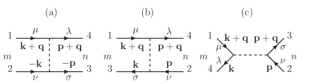
Figure 1: A generic 4-point vertex $\Gamma_{1234}$ is rearranged into $P$-, $C$-, and $D$-channels in (a)-(c), respectively. Here ${\bf k},{\bf q},{\bf p}$ are momenta, $\mu,\nu,\sigma,\lambda$ are spin indices, and $m,n$ denote the form factors. On each side of the diagrams, the spin (and sublattice) labels are absorbed into the form factor labels wherever applicable (see the main text).

Method – Technically this work requires us to generalize the functional renormalization group (FRG) approach frg-general ; frg4iron ; wangLee ; wang to Hamiltonians without spin rotation symmetry. In addition, because the necessity to study small momentum transfer particle-hole scatterings we use a Matsubara frequency rather than momentum cutoff. All calculations are carried out using the singular-mode functional renormalization group (SM-FRG) method.husemann ; wang

Consider a generic fully-antisymmetized irreducible 4-point vertex function $\Gamma_{1234}$ in $\Psi^{\dagger}_{1}\Psi^{\dagger}_{2}(-\Gamma_{1234})\Psi_{3}\Psi_{4}$. Here $1,2,3,4$ represent momentum and spin (and sublattice) indices. Figs.1(a)-(c) are rearrangements of $\Gamma_{1234}$ into the pairing (P), crossing (C) and direct (D) channels each characterized by a collective momentum ${\bf q}$. In each channel the vertex function is decomposed as Eq. (4) of the Appendix. There $\{f_{m}\}$ is a set of orthonormal lattice form factors.formfactor The spin (and sublattice) indices are contained in the label of the form factors as shown in Figs.1(a)-(c). The decomposition in Eq. (4) is exact if the form factors are complete, but a few of them are often enough to capture the leading instabilities.husemann ; wang The FRG flow equations for $P,C$ and $D$ as a function of the cutoff scale $\Lambda$ are given by Eqs.(6),(7) and (8) of the Appendix. The effective interaction in the particle-particle (pp) and particle-hole (ph) channels are given, respectively, by $V_{pp}=-P$ and $V_{ph}=C$. [Because of antisymmetry $D$ ($=-C$) does not yield any new information.] During the FRG flow we monitor the singular values of the matrix functions $V_{pp/ph}({\bf q})$. The most negative singular values, $S_{pp/ph}$, occur at special momenta ${\bf q}_{pp/ph}$. While ${\bf q}_{pp}$ is usually zero, ${\bf q}_{ph}$ can evolve under RG before settling down to fixed values. The eigen function associated with $S_{pp}$ is used to construct the gap function. More technical details can be found in the Appendix.

A strongly correlated one-band model in continuum limit – We consider spin-1/2 fermions hopping on a square lattice. The Hamiltonian is given by

$$H = \sum_{{\bf k}}\Psi^{\dagger}_{{\bf k}}[\epsilon({\bf k}){\sigma}_{0}+\lambda\vec{\gamma}({\bf k})\cdot\vec{{\sigma}}]\Psi_{{\bf k}}$$ (1)

$$+ U\sum_{i}n_{i\uparrow}n_{i\downarrow}+V\sum_{\langle ij\rangle}n_{i}n_{j}=H_{0}+H_{I}.$$

Here $\Psi^{\dagger}=(\psi^{\dagger}_{\uparrow},\psi^{\dagger}_{\downarrow})$, $\epsilon({\bf k})=-2t(\cos k_{x}+\cos k_{y})-\mu$ ($t$ is the nearest neighbor hopping integral and $\mu$ is the chemical potential), $i$ labels the lattice sites, $n_{i\sigma}=\psi^{\dagger}_{i\sigma}\psi_{i\sigma}$ and $n_{i}=\sum_{\sigma}n_{i\sigma}$. In addition, ${\sigma}_{0}$ is the $2\times 2$ identity matrix and $\vec{\sigma}$ denotes the three Pauli matrices. In the following we shall set $U=8t$ and $V=-2t$ for the on-site and nearest neighbor interactions. For the Rashba spin-orbit coupling we consider $\vec{\gamma}({\bf k})=(-\sin k_{y},\sin k_{x},0)$.

Combining the time-reversal and point group ($C_{4v}$ in the present case) symmetries , it can be shown that the Cooper pair operator $B^{\dagger}=\sum_{\bf k}\Psi^{\dagger}_{\bf k}\Delta_{\bf k}\Psi^{{\dagger}T}_{-{\bf k}}$ takes the form,noncentrosymmetric $\Delta({\bf k})=[\phi({\bf k})\sigma_{0}+\vec{d}({\bf k})\cdot\vec{{\sigma}}]i\sigma_{2},$ where $\vec{d}({\bf k})$ transforms, under the point group, like the product of $\phi({\bf k})$ and $\vec{\gamma}({\bf k})$. In the cases we have studied, to a good approximation, we can write

$$\Delta({\bf k})=[\phi({\bf k})\sigma_{0}+\chi({\bf k})\hat{\gamma}({\bf k})\cdot\vec{{\sigma}}]i\sigma_{2},$$ (2)

where $\hat{\gamma}({\bf k})=\vec{\gamma}({\bf k})/|\vec{\gamma}({\bf k})|$, $\phi({\bf k})$ and $\chi({\bf k})$ are even functions of ${\bf k}$ (real up to a global phase) and transform according to the same irreducible representation of the point group (for multi-dimensional representations there are several $\phi$ and $\chi$’s). In Landau theory, $\phi$ and $\chi$ act as order parameters, and can induce each other in the presence of the Rashba coupling ($\lambda\neq 0$).

It is important to note that the Rashba term splits each of the otherwise spin-degenerate Fermi surface into two. The spin split Fermi surfaces are characterized by eigen values $\pm 1$ of $\hat{\gamma}({\bf k})\cdot\vec{{\sigma}}$. In the case where $\phi({\bf k})$ and $\chi({\bf k})$ are nodeless, the gap function on the two split Fermi surfaces will have opposite sign if the magnitudes of $\chi({\bf k})$ dominates over $\phi({\bf k})$. It turns out that for each pair of Fermi pockets surrounding a TRI ${\bf k}$ point the above sign reversal leads to two counter-propagating Majorana edge modes . Thus topological pairing requires the triplet $\chi$-component to be dominant. Moreover sign reversal (in the gap function) on an odd/even pairs of the spin-split Fermi surfaces (satisfying the condition specified above) will lead to strong/weak topological superconductivity.

For $\lambda=0.01t$ and $\mu=-3t$ the spin-split Fermi surfaces are shown in Fig.2(a). The pockets are small, mimicking the continuum limit. The form factors used in our SM-FRG extend up to second neighbors in real space.formfactor The RG flow of $S_{pp/ph}$ are shown in Fig.2(b). During the flow ${\bf q}_{ph}$ evolves from ${\bf q}_{1}=(\pi,\pi)$ and settles down at ${\bf q}_{2}=0$. By inspecting the spin structure of the ${\bf q}_{2}$-singular mode we find it corresponds to ferromagnetic fluctuation. The leading pairing channel is extended $s$-wave at cutoff energies above point A (because the bare $V<0$). But at lower cutoff energies the increased ferromagnetic fluctuation around ${\bf q}_{2}$ enhances pairing in the triplet channel via their mutual overlaps (see Appendix). The cusps at A, B and C associated with the $S_{pp}$ flow is due to the evolution of the leading pairing form factor. The gap function is determined by the singular mode associated with $S_{pp}$ at the diverging cutoff scale. The result is a dominant $\chi$-component together with a much smaller $\phi$-component. The corresponding gap function on the two Fermi surfaces is shown in Fig.2(a) (gray scale). A sign change is clearly visible. According to the established criterion,rev2 this pairing state is topological. To verify this, we calculate the BdG energy spectrum using the obtained pairing form factor in a strip geometry (open-boundary along $\hat{x}$). The resulting eigen energies as a function of $q=k_{y}$ is shown in Fig.2(c). There are two in-gap branches of Majorana edge modes associated with each edge.

Had we turned off the Rashba coupling, the leading pairing channel ($p$-wave) would be two-fold degenerate (with dominant amplitudes on 1st neighbor bonds). Under this condition even an infinitesimal Rashba coupling breaks the degeneracy by linearly recombining the $p$-waves into $\Delta({\bf k})=i\sin k_{x}\sigma_{0}+\sin k_{y}\sigma_{3}$, or $\chi({\bf k})=|\vec{\gamma}({\bf k})|$ in Eq.(2), leading to a gap function $\pm\chi({\bf k})$ on the infinitesimally split Fermi surfaces. This gap function has the same symmetry as the two dimensional version of the ³He B phase. In fact there are strong similarities between the model (and its properties) described above and the B phase of ³He. For example The small filling fraction enables this model to describe the continuum limit. The strong on-site repulsion mimics the short-range strong repulsive correlation in ³He, while the weaker nearest neighbor attraction is a caricature of the tail of the Lennard-Jones potential. The enhanced ferromagnetic fluctuation and the resulting triplet pairing is consistent with the pairing mechanism described by Anderson and Brinkmanab . In addition, the Rashba coupling plays a similar role as the parity -invariant spin-orbit interaction in ³He: they both lift the degeneracy in the pairing channel.

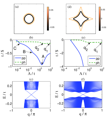
Figure 2: (Color online) Left panels: Results for the toy model of He³. (a) The Fermi pockets and the associated gap functions (gray scale, in units of $t$). The spin-splitting between the pockets is enlarged for clarity. The box is the zone boundary. (b) The SM-FRG flow of $S_{pp/ph}$ versus cutoff scale $\Lambda$. Arrows mark sharp changes in the RG evolution. (c) The low energy BdG eigen spectrum in a strip (open along $\hat{x}$) as a function of the momentum $q\hat{y}$. Right panels: the same plots as in the left panels but for a model whose Fermi surfaces are in proximity to van Hove singularities.

Topological pairing in the vicinity of van Hove singularity– In this section we demonstrate that topological pairing can be enhanced when the Fermi surfaces are close to van Hove singularities. Here we set $V=0$ (so that the interaction is purely repulsive), and add a 2nd neighbor hopping $t^{\prime}$ so that $\epsilon({\bf k})=-2t(\cos k_{x}+\cos k_{y})-4t^{\prime}\cos k_{x}\cos k_{y}-\mu$. For $t^{\prime}=-0.475t$, $\mu=-2t$ and $\lambda=0.01t$, the spin-split Fermi surfaces are shown in Fig.2(d). They are pointy along $\hat{x}$ and $\hat{y}$ reflecting the existence of saddle points (van Hove singularities) on the Brillouin zone boundary. These features lead to enhanced ferromagnetic correlations via the Stoner mechanism. As a consequence triplet pairing is enhanced and the diverging scale of $S_{pp}$ is raised. These are shown in Fig.2(e) for $U=2.5t$. The arrows associated with the $S_{ph}$ flow record the ${\bf q}_{ph}$ evolution from ${\bf q}_{1}=(\pi,\pi)$ to ${\bf q}_{2}=0$. As in the previous section, this implies ferromagnetic correlations at low energies. The final gap function on the Fermi surfaces are shown in Fig.2(d) (gray scale), again with desired sign reversal. Such a pairing function leads to the BdG energy spectrum shown in Fig.2(f) in a strip geometry. The edge modes are apparent.

Topological pairing enhanced by inter-pocket scattering – In this section we show a third route to topological pairing. In this case pairing is triggered by inter-Fermi surface scattering in a way similar to the pairing in the pnictidesfrg4iron ; wangLee .

Consider a honeycomb lattice. The single particle Hamiltonian is given by

$$H_{0}= -\sum_{i\delta}\Psi_{i}^{\dagger}t_{\delta}\Psi_{i+\delta}-i\lambda\sum_{i\delta_{nn}}\Psi^{\dagger}_{i}(\hat{z}\times\vec{\delta}_{nn}\cdot\vec{{\sigma}})\Psi_{i+\delta_{nn}}$$ (3)

$$-\mu\sum_{i}\Psi^{\dagger}_{i}\Psi_{i}.$$

Here $i$ labels lattice sites, $\delta$ runs over the 1st and 2nd neighbor bonds, with $t_{\delta}=t,t^{\prime}$. The spin-dependent hopping, the Rashba term, is limited to the nearest neighbor bonds $\delta_{nn}$. Choosing a lattice site as the origin, the point group is $C_{3v}$. For the SM-FRG calculation, we choose the form factors up to the 2nd neighbors.formfactor (Since the honeycomb lattice has two sites per unit cell the labels of the form factors in Fig.1 include the sublattice indices.wang .) The Fermi surfaces for $t^{\prime}=0.357t$, $\lambda=0.02t$ and $\mu=1.664t$ are shown in Fig.3(a). There are a few interesting features of the band structure that are worth noting (1) The Fermi surfaces encircle either the zone center ($\Gamma$) or the zone corners (K and K^′). However only $\Gamma$ is TRI, hence according to Ref.rev2 only the $\Gamma$-Fermi surfaces are topologically relevant. (2) The $\Gamma$ and K-pockets have close by segments, hence allow small momentum transfer particle-hole scattering. If such scattering is magnetic, it corresponds to nearly ferromagnetic fluctuations, hence can induce triplet and topological pairing.

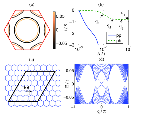
Figure 3: (Color online) (a) The Fermi pockets and the associated gap functions (gray scale, in units of $t$). The spin-splitting between each pair of Fermi pockets is enlarged for clarity. The hexagon is the zone boundary. (b) The SM-FRG flow of $S_{pp/ph}$ versus the cutoff scale $\Lambda$. Arrows mark sharp changes of ${\bf q}_{ph}$ during the RG flow. (c) A strip (marked by the thick lines) open along ${\bf a}$ and periodic along ${\bf b}$ directions (${\bf a}$ and ${\bf b}$ are primitive lattice vectors). (d) The low energy BdG eigen spectrum for (c) as a function of the conserved momentum $q$ along ${\bf b}$.

In the following we show for $U=1.26t$ this is exactly what happens. During the RG flow shown in Fig.3(b), the strength of $S_{ph}$ increases and ${\bf q}_{ph}$ evolves from ${\bf q}_{1}=(0.667,1.152)\pi$ to ${\bf q}_{2}=0$, ${\bf q}_{3}=(0.250,0.048)\pi$ and finally settles down at ${\bf q}_{4}=(0.333,0.192)\pi$. We have checked that ${\bf q}_{4}$ corresponds to the scattering between near by parallel segments between the $\Gamma$ and K pockets. Inspection of the spin structure of the singular mode associated with ${\bf q}_{2,3,4}$ reveals that they corresponds to spin fluctuations. As such fluctuations are enhanced, they causes $S_{pp}$ to grow in magnitude and eventually diverge at a relatively high critical scale. The resulting gap function is shown in Fig.3(a) in gray scale. It is fully gapped on all Fermi surfaces, and have opposite sign on each pair of spin-split pockets. Since the K-pockets are topologically irrelevant, the sign change between the $\Gamma$ Fermi surfaces implies the pairing is strong-topological. To verify this we consider a strip schematically shown in Fig.3(c). It is open along ${\bf a}$ and periodic along ${\bf b}$ directions. The BdG energy spectrum as a function of the momentum $q={\bf k}\cdot\hat{b}$ is shown in Fig.3(d). There are two branches of Majorana modes at each edge.

Thus in all of the above examples we have seen small momentum magnetic fluctuations $\Rightarrow$ degenerate triplet pairing, and degenerate triplet pairing + Rashba coupling $\Rightarrow$ topological pairing. The fact that ferromagnetic fluctuations enhance triplet pairing has a long history. These include the works on the pairing of ³He,helium , and the extension of the Kohn-Luttinger theorem to $p$-wave pairing for 2D and 3D electron gas in the dilute limit.fl ; chub For lattice systems, a 2D Hubbard model with large enough 2nd neighbor hopping has been shown to exhibit $p$-wave pairing for small band fillings.2dh

Finally, if pairing is singlet in the absence of spin-orbit interaction a weak Rashba coupling only induces a small triplet component, hence is insufficient to induce the desired sign change in the gap function. Of course this does not rule out the possibility of topological pairing in the presence of strong spin-orbit interaction.

In conclusion through the study of the above three, and many other not included, examples we conclude that TRI topological superconductivity in symmetry class DIII should occur in systems close to the ferromagnetic (or small wavevector magnetic) instability. Bandstructure wise, in the absence of Rashba coupling, these systems should have an odd number of spin-degenerate Fermi pockets (each enclosing a TRI momentum) in order for strong topological pairing to occur.

I Appendix

In the supplementary material, we provide the technical details of the SM-FRG method.wang .

We begin by reviewing the definition of the vertex functions used in the main text. Consider a generic fully-antisymmetized irreducible 4-point vertex function $\Gamma_{1234}$ in $\Psi^{\dagger}_{1}\Psi^{\dagger}_{2}(-\Gamma_{1234})\Psi_{3}\Psi_{4}$. Here $1,2,3,4$ represent momentum and spin (and sublattice) indices. Figs.4(a)-(c) are rearrangements of $\Gamma_{1234}$ into the pairing (P), crossing (C) and direct (D) channels each characterized by a collective momentum ${\bf q}$. The rest momentum dependence of the vertex function can be decomposed as,

$$\Gamma_{{\bf k}+{\bf q},-{\bf k},-{\bf p},{\bf p}+{\bf q}}^{\mu\nu\sigma\lambda}\rightarrow\sum_{mn}f_{m}^{*}({\bf k})P_{mn}({\bf q})f_{n}({\bf p}),$$

$$\Gamma_{{\bf k}+{\bf q},{\bf p},{\bf k},{\bf p}+{\bf q}}^{\mu\nu\sigma\lambda}\rightarrow\sum_{mn}f_{m}^{*}({\bf k})C_{mn}({\bf q})f_{n}({\bf p}),$$

$$\Gamma_{{\bf k}+{\bf q},{\bf p},{\bf p}+{\bf q},{\bf k}}^{\mu\nu\sigma\lambda}\rightarrow\sum_{mn}f_{m}^{*}({\bf k})D_{mn}({\bf q})f_{n}({\bf p}).$$ (4)

Here $\{f_{m}\}$ is a set of orthonormal lattice form factors. The spin (and sublattice) indices are contained in the label of the form factors as shown in Figs.4(a)-(c). The decomposition in Eq. (4) is exact if the form factors are complete, but in practice a few of them are often enough to capture the leading instabilities.husemann ; wang Because of full antisymmetry, the matrices $C$ and $D$ satisfy $D=-C$, and are therefore not independent. In the following $D$ is used for bookkeeping purpose.

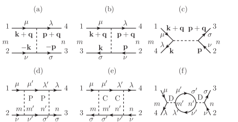
Figure 4: A generic 4-point vertex $\Gamma_{1234}$ is rearranged into $P$-, $C$-, and $D$-channels in (a)-(c), respectively. Here ${\bf k},{\bf q},{\bf p}$ are momenta, $\mu,\nu,\sigma,\lambda$ denote spins, and $m,n$ denote the form factors. On each side of the diagrams, the spin (and sublattice) labels are absorbed into the form factor labels wherever applicable. The one-loop diagrams that contribute to $\partial P$, $\partial C$ and $\partial D$ are shown in (d)-(f), respectively.

Ignoring the spin and sublattice labels for the moment, the form factors are given by

$$f_{m}({\bf k})=\sum_{{\bf r}}f_{m}({\bf r})\exp(-i{\bf k}\cdot{\bf r}),$$ (5)

where $f_{m}({\bf r})$ transforms according to an irreducible representation of the point group, and ${\bf r}$ is the bond vectors connecting the two $\Psi$’s (or two $\Psi^{\dagger}$’s) in Fig.4(a) and one $\Psi$ and one $\Psi^{\dagger}$ in Fig.4(b) and (c). In our calculation we choose form factors up to the 2nd neighbor bonds. We have checked that longer range form factors does not change the results qualitatively. To be specific, for square lattice, the real-space form factors we used are 1) $f_{1}=1$ for on-site; 2) $f_{2}=1/2$, $f_{3}=(1/2)\cos 2\theta_{\bf r}$, $f_{4}=\sqrt{1/2}\cos\theta_{\bf r}$, and $f_{5}=\sqrt{1/2}\sin\theta_{\bf r}$ for 1st neighbors, where $\theta_{\bf r}$ is the azimuthal angle of ${\bf r}$; 3) $f_{6}=1/2$, $f_{7}=(1/2)\sin 2\theta_{\bf r}$, $f_{8}=\sqrt{1/2}\cos(\theta_{\bf r}-\pi/4)$ and $f_{9}=\sqrt{1/2}\sin(\theta_{\bf r}-\pi/4)$ for 2nd neighbors. For hexagonal lattices, the form factors we used are 1) $f_{1}=1$ for on-site; 2) $f_{2}=\sqrt{1/3}$, $f_{3}=\sqrt{2/3}\cos\theta_{\bf r}$ and $f_{4}=\sqrt{2/3}\sin\theta_{\bf r}$ for 1st neighbors; 3) $f_{5}=\sqrt{1/6}$, $f_{6}=\sqrt{1/3}\cos\theta_{\bf r}$, $f_{7}=\sqrt{1/3}\sin\theta_{\bf r}$, $f_{8}=\sqrt{1/3}\cos 2\theta_{\bf r}$, $f_{9}=\sqrt{1/3}\sin 2\theta_{\bf r}$, $f_{10}=\sqrt{1/6}\cos 3\theta_{\bf r}$ for 2nd neighbors. Notice that the 1st neighbor bonds stem from different sublattices are negative to each other.

In the case where sublattices are involved, the form factor label $m$ also includes the sublattice indices associated with the two $\Psi$’s (or $\Psi^{\dagger}$’s), or the $\Psi$ and $\Psi^{\dagger}$. However, once ${\bf r}$ is fixed only one of these sublattice indices is independent. We include the independent sublattice index in the form factor label, $(m,a)\rightarrow m$. Here $a$ labels, e.g., the fermion field 1 or 4 in Fig.4(a), 1 or 4 in (b), and 1 or 3 in (c). The sublattice index is an independent label because point group operations do not mix sublattices when the origin is chosen to be a lattice site.

The total number of form factors $N$ in a calculation is determined by the number of real space neighbors, the number of sublattices and the four spin combinations $(\mu,\nu)=\uparrow\uparrow,\uparrow\downarrow,\downarrow\uparrow,\downarrow\downarrow$ associated with two $\Psi$ (P channel) or the $\Psi$ and $\Psi^{\dagger}$ (C and D channels). Thus $P$, $C$ and $D$ are all $N\times N$ matrix functions of momentum ${\bf q}$.

The Feynman diagrams associated with one-loop contributions to the flow of the irreducible 4-point vertex function are given in Fig.4(d)-(f). They represent the partial changes $\partial P$, $\partial C$ and $\partial D$, respectively. (Notice that the three diagrams in Fig.4(d)-(f) become the usual five diagrams in the spin-conserved case.) The internal Greens functions are convoluted with the form factors hence in matrix form,

$$\partial P/\partial\Lambda=P\chi^{\prime}_{pp}P/2,$$

$$\partial C/\partial\Lambda=C\chi^{\prime}_{ph}C,$$

$$\partial D/\partial\Lambda=-D\chi_{ph}^{\prime}D,$$ (6)

where we have suppressed the dependence of the collective momentum ${\bf q}$, and

$$(\chi^{\prime}_{pp})_{mn} =\frac{\partial}{\partial\Lambda}\int\frac{d{\omega}_{n}}{2\pi}\int\frac{d^{2}{\bf p}}{S_{BZ}}f_{m}({\bf p})G({\bf p}+{\bf q},i{\omega}_{n})G(-{\bf p},-i{\omega}_{n})f_{n}^{*}({\bf p})\theta(|{\omega}_{n}|-\Lambda)$$

$$=-\frac{1}{2\pi}\int\frac{d^{2}{\bf p}}{S_{BZ}}f_{m}({\bf p})G({\bf p}+{\bf q},i\Lambda)G(-{\bf p},-i\Lambda)f_{n}^{*}({\bf p})\ \ +(\Lambda\rightarrow-\Lambda),$$

$$(\chi^{\prime}_{ph})_{mn} =\frac{\partial}{\partial\Lambda}\int\frac{d{\omega}_{n}}{2\pi}\int\frac{d^{2}{\bf p}}{S_{BZ}}f_{m}({\bf p})G({\bf p}+{\bf q},i{\omega}_{n})G({\bf p},i{\omega}_{n})f_{n}^{*}({\bf p})\theta(|{\omega}_{n}|-\Lambda)$$ (7)

$$=-\frac{1}{2\pi}\int\frac{d^{2}{\bf p}}{S_{BZ}}f_{m}({\bf p})G({\bf p}+{\bf q},i\Lambda)G({\bf p},i\Lambda)f_{n}^{*}({\bf p})\ \ +(\Lambda\rightarrow-\Lambda),$$

where $G$ is the free fermion Greens function, $S_{BZ}$ is the total area of the Brillouine zone. Here $\Lambda>0$ is the infrared cutoff of the Matsubara frequency ${\omega}_{n}$. As in usual FRG implementation, the self energy correction and frequency dependence of the vertex function are ignored.

Since $\partial P$, $\partial C$ and $\partial D$ come from independent one-loop diagrams, they contribute independently to the full $d\Gamma_{1234}$, which needs to be projected onto the three channels. Therefore the full flow equations are given by, formally,

$$dP/d\Lambda=\partial P/\partial\Lambda+\hat{P}(\partial C/\partial\Lambda+\partial D/\partial\Lambda),$$

$$dC/d\Lambda=\partial C/\partial\Lambda+\hat{C}(\partial P/\partial\Lambda+\partial D/\partial\Lambda),$$

$$dD/d\Lambda=\partial D/\partial\Lambda+\hat{D}(\partial P/\partial\Lambda+\partial C/\partial\Lambda),$$ (8)

where $\hat{P},\hat{C}$ and $\hat{D}$ are the projection operators in the sense of Eq. (4). Here we have used the fact that $\hat{K}(\partial K)=\partial K$ for $K=P,C,D$. In Eq. (8) the terms preceded by the projection operators represent the overlaps of different channels. For two channels to overlap, the spatial coordinates of all four fermion fields must lie within the range set of the form factors. In the actual calculation the projections in Eq.(8) are preformed in real space.

The effective interaction in the particle-particle (pp) and particle-hole (ph) channels are given, respectively, by $V_{pp}=-P$ and $V_{ph}=C$. By singular value decomposition, we determine the leading instability in each channel,

$$V_{X}^{mn}({\bf q}_{X})=\sum_{\alpha}S_{X}^{\alpha}\phi_{X}^{\alpha}(m)\psi_{X}^{\alpha}(n),$$ (9)

where $X=pp,ph$, $S_{X}^{\alpha}$ is the singular value of the $\alpha$-th singular mode, $\phi_{X}^{\alpha}$ and $\psi_{X}^{\alpha}$ are the right and left eigen vectors of $V_{X}$, respectively. We fix the phase of the eigen vectors by requiring ${\rm Re}[\sum_{m}\phi_{X}^{\alpha}(m)\psi_{X}^{\alpha}(m)]>0$ so that $S_{X}^{\alpha}<0$ corresponds to an attractive mode in the X-channel.

In the pp-channel ${\bf q}_{pp}=0$ corresponds to the zero center-of-mass momentum Cooper instability. The matrix gap function $\Delta_{{\bf k}}$ in the spin and sublattice basis is determined as follows. A singular mode $\phi_{pp}^{\alpha}$ leads to a pair operator (in the momentum space),

$$\Psi^{\dagger}_{\bf k}\Delta_{\bf k}\Psi^{{\dagger}T}_{-{\bf k}}=\sum_{m=(m,a,\mu,\nu)}\psi_{a\mu}^{\dagger}({\bf k})\phi_{pp}^{\alpha}(m)f_{m}({\bf k})^{*}\psi_{a_{m}\nu}^{\dagger}(-{\bf k}).$$ (10)

Here $a$ is the independent sublattice index, and $a_{m}$ is the second sublattice index determined by $a$ and $m$ as discussed earlier, and $\mu,\nu$ are spin indices. The parity of $\Delta_{\bf k}$ under space inversion determines the singlet and triplet components. The gap function in the band eigen basis can be determined by the unitary transformation

$$\tilde{\Psi}^{\dagger}_{\bf k}=\Psi^{\dagger}_{\bf k}U^{\dagger}_{\bf k},$$ (11)

where the columns of $U^{\dagger}_{\bf k}$ are the Bloch states $\{|{\bf k},n\rangle\}$ ($n$ is the band index). Under Eq. (11) the pairing matrix transforms into

$$\tilde{\Delta}_{\bf k}=U_{\bf k}\Delta_{\bf k}U_{-{\bf k}}^{T}.$$ (12)

In the weak coupling case (i.e., when the magnitude of the superconducting gap is much smaller than the bandwidth), only the diagonal part of $\tilde{\Delta}$ (i.e., intra-Fermi surface pairing) is important. Since Eq. (12) involves Bloch states at two different momenta, the phases of the associated Bloch states enters $\tilde{\Delta}$. Since there is time-reversal symmetry we fix the Bloch state phase at ${\bf k}$ and $-{\bf k}$ by demanding $\hat{T}|{\bf k},n\rangle=|-{\bf k},n\rangle$ and $\hat{T}^{2}|{\bf k},n\rangle=-|{\bf k},n\rangle$, where $\hat{T}=i\sigma_{2}K$ is the time-reversal operator.

In the particle-hole channel, we calculate the singular values associated with $V_{ph}({\bf q})$ at all momenta ${\bf q}$. Unlike the Col[oooper channel, the most negative singular value can occur at non-zero momentum ${\bf q}_{ph}$. The associated particle-hole operator is given by

$$\Psi^{\dagger}_{{\bf k}+{\bf q}}\Pi_{\bf k}\Psi_{\bf k}=$$

$$\sum_{m=(m,a,\mu,\nu)}\psi_{a\mu}^{\dagger}({\bf k}+{\bf q})\phi_{ph}^{\alpha}(m)f^{*}_{m}({\bf k})\psi_{a_{m}\nu}({\bf k}).~{}$$ (13)

Usually the on-site form factor dominates in the particle-hole channel. By inspecting the spin structure of the on-site form factor one can easily determine whether the instability is charge or spin like.