A CDS Option Miscellany

Abstract

CDS options allow investors to express a view on spread volatility and obtain a wider range of payoffs than are possible with vanilla CDS. The authors give a detailed exposition of different types of single-name CDS option, including options with upfront protection payment, recovery options and recovery swaps, and also presents a new formula for the index option. The emphasis is on using the Black’76 formula where possible and ensuring consistency within asset classes. In the framework shown here the ‘armageddon event’ does not require special attention.

First version: Dec 2009

Second version: Jul 2017 (index option section updated)

This version: Apr 2019 (minor corrections)

1 Introduction

CDS options allow investors to express a view on spread volatility and give a wider range of payoffs than are possible with vanilla CDS. Index options are commonly traded: the reader is referred to [7] for a discussion of trading strategies and hedging of index options. The market in the single-name options is not well developed, but the options are embedded in a number of structured products, for example cancellable single-name protection. With the standardisation of the single-name CDS and the move to central clearing, and the greater emphasis placed on hedging and CVA, it is possible that single-name CDS options will become more relevant, in the same way that equity options have been around for years. Accordingly, their definition and valuation merits study.

The valuation of single-name options with running spread was originally performed in the Black’76 framework some years ago [9, 13, 14]. In this article we briefly review it and develop the subject to point out what happens when the strike is part-upfront, by which we mean that on exercise the CDS protection is to be paid wholly or partly upfront rather than all-running—which is how contracts now trade. Upfronts introduce complications. The Black’76 formula is not directly applicable because on exercise the option is not being paid for in units of risky annuity, but instead in a mixture of cash and risky annuity. We could simply start with a hazard rate model formulation, and build everything up from first principles. This is the approach taken by more recent authors such as [1, 3]. However, we would lose equivalence with Black76 in the all-running case, even for a lognormal hazard rate model. (Lognormal hazard rate dynamics do not exactly correspond to lognormal credit spreads. Also, in the all-running case the spread is assumed for mathematical convenience to be lognormal in the survival measure with the risky PV01 as numeraire, not the money market account.) We wish to keep consistency with Black’76 as far as possible as that is the standard model used on trading desks, even if Brownian spread dynamics are ‘clearly not right’. Another complication of upfronts is that the no-knockout option contains an embedded option on realised recovery, for which pricing models need to be developed. We deal with this too.

CDS indices are different from single-name options in that they trade no-knockout: the payoff arising from defaults in the life of the option is referred to as front-end protection (FEP). It is pointed out by Pedersen [11] that one cannot simply add the FEP to a knockout payer option to get the no-knockout price: the exercise decision depends on the accrued loss. He addresses this problem by introducing a loss-adjusted spread which he then models as lognormal. But Brigo ([4] & references therein) points out that spread-based formulae have a problem: to derive them rigorously requires changing numeraire to the associated PV01. In the ‘armageddon’ event of all names defaulting, the numeraire collapses to zero and the spread becomes undefined, so this event has to be conditioned against and treated separately. Brigo & Morini seek to estimate the probability of collapse using the tranche market, but this market has hardly been a paragon of efficiency, and they use the Gaussian copula model which did not even calibrate during the crisis: also, what is one to do with an index on which no tranches are traded (e.g. ITX.XO)?

Most academic literature, including [4, 12, 15, 8], fails to treat the payoff of a CDS index option correctly. A CDS index is not a portfolio of par single name CDS: it trades upfront with a fixed coupon and in the options the form of the strike leg payment needs careful attention. In fact, Rutkowski & Armstrong [12, Eq.42] start by writing down the payoff correctly, then remark that it is difficult to handle analytically (which is true) and that it is “internally inconsistent” (as we explain later, it is not) and then proceed to model something else instead. With the exception of that paper, it appears that academic authors are unaware of how credit instruments trade, and so they end up (inventing and then) solving rather uninteresting problems. For example, Herbertsson’s assertion [8] that lognormal distributions are not ideal is, in common with other areas of finance, correct, but introducing significant extra complexity into a model and making pronouncements about real-world pricing seems to be of dubious value when the equation for the instrument’s payoff [8, Eq.(2.3.1)] is incorrect at the outset. Of the practitioner literature, Pedersen [11] and O’Kane [10] get it right, though O’Kane’s exposition is clearer. As a general rule it is best to regard a CDS index option as physically settled, i.e. it exercises into an index CDS contract, even if the resulting contract is immediately closed out. In other words it is not a ‘spread option’ but rather an option on a contract PV. In fact, the ‘armageddon event’ is not a difficulty in our framework, and so one does not need to estimate its probability, which is just as well as such a procedure would be little better than guesswork.

Notation. RPV01 means the PV of a risky annuity (IO strip) on the issuer; the symbol for its value on date $t$ will be $V^{1}_{t}(T_{1},T_{2})$, indicating the dates $T_{1},T_{2}$ between which the annuity is to be paid. The value of the annuity collapses to 0 on default. By the ‘default-PV’ of a CDS, $V^{D}_{t}(T_{1},T_{2})$, we mean the PV of the protection leg. As usual $B$ denotes the riskfree discount factor (riskfree zero-coupon bond price), $\mathfrak{B}_{t}$ the rolled-up money market account ($\mathfrak{B}_{0}=1$), and for single issuers $\tau$ is the default time and $Q(t)$ the survival probability. $C_{+},C_{-}$ generically denote a call or put on some underlying, the interpretation being obvious from the context.

2 Single-name options

2.1 Knockout, running

In the old days, single-name options have been assumed to trade knockout and exercise into protection paid as a running premium. The payer price $C_{+}$ (the receiver price will be analogous and we omit it throughout to save space) is

$$C_{+}^{\textrm{ko,r}} = \mathbf{E}_{0}\left[\frac{1}{\mathfrak{B}_{t_{E}}}\big{(}V^{D}_{t_{E}}(t_{E},T)-s_{K}V^{1}_{t_{E}}(t_{E},T)\big{)}^{+}\mathbf{1}(\tau>t_{E})\right]$$

$$= \mathbf{E}_{0}\!\left[(\overline{s}_{t_{E}}-s_{K})^{+}V^{1}_{t}(t_{E},T)\right]$$

where $\overline{s}$ denotes the par spread, $s_{K}$ the strike spread, $V^{1}_{t}$ the RPV01, $t_{E}$ the expiry date of the option, and $T$ the maturity date of the underlying swap (today=0). Now $V_{t}^{1}$ is a collapsing numeraire as it is zero after default, so we pass to the survival measure [14] $\mathbf{E}^{*}$ defined as

$$\mathbf{E}^{*}[Z]\equiv\frac{\mathbf{E}[\mathfrak{B}_{t_{E}}^{-1}ZV^{1}(t_{E},T)\mathbf{1}(\tau>t_{E})]}{\mathbf{E}[\mathfrak{B}_{t_{E}}^{-1}V^{1}(t_{E},T)\mathbf{1}(\tau>t_{E})]};$$

note that in the denominator the survival indicator is unnecessary as $V^{1}_{t}=0$ if default occurs before time $t$. Then

$$C_{+}^{\textrm{ko,r}}=\mathbf{E}^{*}_{0}\left[(\overline{s}_{t_{E}}-s_{K})^{+}\right]V^{1}_{0}(t_{E},T).$$

Under $\mathbf{E}^{*}_{0}$, $\overline{s}_{t}$ is assumed to be lognormal, and then the expectation evaluates using Black’76 to get:

$$C_{+}^{\textrm{ko,r}}=\big{(}\overline{s}_{F}\Phi(d_{+})-s_{K}\Phi(d_{-})\big{)}V^{1}_{0}(t_{E},T)$$ (1)

$$d_{\pm}=\displaystyle\frac{\ln(\overline{s}_{F}/s_{K})\pm\frac{1}{2}\sigma^{2}t_{E}}{\sigma\sqrt{t_{E}}}.$$

Note that $\overline{s}_{F}$ (the knockout forward spread) is equal to $V^{D}_{0}(t_{E},T)/V^{1}_{0}(t_{E},T)$ until default, at which point it becomes undefined. When performing any statistical analysis on the credit spread, for example to estimate realised volatility, one is naturally observing it prior to default anyway, so the survival measure is the natural frame of reference.

2.2 No-knockout, running

A no-knockout option remains valid after default. By splitting it into a survival-contingent and a default-contingent part, one sees that the NKO payer must be worth the sum of the KO payer option and the FEP, so

$$C_{+}^{\textrm{nko,r}}=C_{+}^{\textrm{ko,r}}+V^{D}_{0}(0,t_{E}).$$

A NKO receiver option is worth no more than a knockout receiver option because a receiver option is never exercised into a defaulted credit: one would receive no running spread but pay par minus recovery. However, if the premium leg on exercise is partly paid upfront, the position is more difficult, as we are about to see.

2.3 Knockout, upfront+running

If the premium on exercise is to be paid partly (or wholly) upfront, the expression for the payer option is now

$$C_{+}^{\textrm{ko,ur}}=\mathbf{E}_{0}\!\left[\frac{1}{\mathfrak{B}_{t_{E}}}\big{(}V^{D}_{t_{E}}(t_{E},T)-u_{K}-s_{K}V^{1}_{t_{E}}(t_{E},T)\big{)}^{+}\mathbf{1}(\tau>t_{E})\right]$$ (2)

where $u_{K}$ is the upfront part of the strike and $s_{K}$ is the running part (in practice this is likely to be 100bp or 500bp). The RPV01 in the strike leg is as before and at maturity it depends on $\overline{s}_{t_{E}}$.

If we change numeraire in the same way as before and try to use

$$u_{K}+s_{K}V^{1}_{t}(t_{E},T)$$

as numeraire, we end up with a valid option-pricing formula, but there are some problems. The main one is that it is inconsistent with the previous setup to the extent that one cannot use the same volatility for both. Of the two PV ratios

$$\left(\frac{V^{D}_{0}(t_{E},T)}{s_{K}V^{1}_{0}(t_{E},T)}\right)\mbox{ and }\left(\frac{V^{D}_{0}(t_{E},T)}{u_{K}+s_{K}V^{1}_{0}(t_{E},T)}\right),$$

(conditionally on no default) the former has higher volatility, for when the default-PV goes up, the RPV01 goes down. We therefore expect a CDS option with a strike quoted partly upfront to be worth less than that of an all-running one, all other things being equal. Another objection is that the second quantity is bounded, whereas the first is not, as $s_{t}\to\infty$, so a lognormal distribution is arguably inappropriate; however this should only be an objection for very high strikes.

To ensure consistency with (1) we therefore need to stick with lognormal spread dynamics in the $V^{1}_{t}$-measure (which we are calling $\mathbf{P}^{*}$). However, the direct computation of the option price (2) has to be done in the $\mathfrak{B}_{t}$-measure $\mathbf{P}$. A change of numeraire is required. Under $\mathbf{P}^{*}$ the spread is lognormal, so the expectation of some function $G$ of the spread at time $t$ is

$$\mathbf{E}^{*}_{0}[G(s_{t})]=\int_{-\infty}^{\infty}G\big{(}\overline{s}_{t}(z)\big{)}\phi(z)\,dz,\qquad\overline{s}_{t}(z)=\overline{s}_{F}e^{\sigma z\sqrt{t}-\frac{1}{2}\sigma^{2}t}$$

with $\phi(z)=\frac{1}{\sqrt{2\pi}}\exp(-\frac{1}{2}z^{2})$ and $\overline{s}_{F}$ denoting the forward spread. (Clearly this prescription allows the model to be embedded in a Markovian spread model, which is necessary for term structure models but not for the one-period models here.) Next, note that for any random variable $Z$,

$$\mathbf{E}\!\left[\frac{Z}{\mathfrak{B}_{t}}\mathbf{1}(\tau>t)\right]\equiv\mathbf{E}^{*}\!\left[\frac{Z}{V^{1}_{t}}\right]\mathbf{E}\!\left[\frac{V^{1}_{t}}{\mathfrak{B}_{t}}\mathbf{1}(\tau>t)\right].$$ (3)

We need to link the RPV01 to the spread, i.e. write $V^{1}$ as a function of $\overline{s}$, and to do this we use the standard RPV01 calculation $\widetilde{\Pi}$ based on a flat hazard rate curve and constant ‘assumed’ (or marking) recovery rate $\Re$. For a flat riskfree curve this is

$$\widetilde{\Pi}(s;t,T)=\frac{1-e^{-[r+(1+\varepsilon)s/(1-\Re)](T-t)}}{r+(1+\varepsilon)s/(1-\Re)}$$ (4)

The parameter $\varepsilon$, which is small, will be explained presently. First, set $Z\equiv 1$ in (3) to obtain

$$\int_{-\infty}^{\infty}\frac{\phi(z)\,dz}{\widetilde{\Pi}\big{(}\overline{s}_{t_{E}}(z);t_{E},T\big{)}}=\frac{B^{*}(t_{E})}{V^{1}_{0}(t_{E},T)}$$

in which the RHS is obtained from today’s CDS curve and $B^{*}(t_{E})$ is the risky discount factor. The purpose of $\varepsilon$ is to ensure that this relation is satisfied exactly, and a unique $\varepsilon$ can always be found to do the job. Therefore we have matched the default and premium legs of today’s CDS curve, by matching the forward rate and RPV01. We now have

$$\mathbf{E}_{0}\!\left[\frac{G(\overline{s}_{t_{E}})}{\mathfrak{B}_{t}}\mathbf{1}(\tau>{t_{E}})\right]=\frac{\int_{-\infty}^{\infty}\big{[}G\big{(}\overline{s}_{t_{E}}(z);t_{E},T\big{)}\big{/}\widetilde{\Pi}\big{(}\overline{s}_{t_{E}}(z);t_{E},T\big{)}\big{]}\phi(z)\,dz}{B^{*}(t_{E})/V^{1}_{0}(t_{E},T)}$$ (5)

and can now calculate the option price numerically from (5). This will give consistency with the Black’76 formula, because if the option exercises into all-running protection then the integral (5) gives the same result as (1).

2.4 Knockout, Standard American/European

CDS are now quoted running but trade upfront with a fixed coupon $c$ say. This is very much like the previous section, but the RPV01 is slightly different. There is no standard convention for the options, and the payoff is best written:

$$C_{+}^{\textrm{ko,ur}}=\mathbf{E}_{0}\!\left[\frac{1}{\mathfrak{B}_{t_{E}}}\big{(}(s^{q}_{t_{E}}-c)\widetilde{\Pi}_{t_{E}}(s^{q}_{t_{E}};t_{E},T)-(s_{K}-c)\widetilde{\Pi}_{t_{E}}(s_{?};t_{E},T)\big{)}^{+}\mathbf{1}(\tau>t_{E})\right]$$ (6)

where the notation $s^{q}$ indicates the quoted spread, as distinct from the par spread $\overline{s}$ [the two are related by $(s^{q}-c)\widetilde{\Pi}=(\overline{s}-c)V^{1}$]. The symbol $s_{?}$ in the strike RPV01 reflects uncertainty as to what spread to use: it could be the spot at expiry ($s^{q}_{t_{E}}$) or the strike spread ($s_{K}$). Whichever one is chosen, equation (5) can be used to value the option via a numerical integral. In this way we ensure consistency between the old-style CDS and the new-style with different coupons.

2.5 No-knockout, upfront+running

When part of the CDS premium on exercise is to be paid upfront, the no-knockout receiver option has more value than the knockout. This is because the holder of a receiver owns a call on the realised recovery $\Re$, with strike equal to 100% minus the upfront. For example if the receiver is struck at 12% plus 500bp running, and a default occurs with 92% recovery, the option holder can exercise and make 4%. Similarly the payer has an embedded put:

$$C_{+}^{\textrm{nko,ur}} = C_{+}^{\textrm{ko,ur}}+C_{-}(\Re;1-u_{K})$$

$$C_{-}^{\textrm{nko,ur}} = C_{-}^{\textrm{ko,ur}}+C_{+}(\Re;1-u_{K}).$$

One therefore has the task of valuing the recovery option.

2.6 Recovery swaps and options

Recovery is obviously bounded to $[0,1]$ so we wish to choose an appropriate distributional assumption. Although a Beta distribution is often suggested, we suggest the use of a Vasicek distribution instead as these are a little more tractable, in the sense that for option pricing one only needs the bivariate Normal distribution as opposed to the incomplete Beta function. Also the use of the Vasicek distribution ties in neatly with probit modelling of recovery rates. The recovery $\Re$ is modelled as a transformation of a Normal variable, thus:

$$\Re(Z)=\Phi\!\left(\frac{a+bZ}{\sqrt{1-b^{2}}}\right),\qquad Z\sim N(0,1)$$

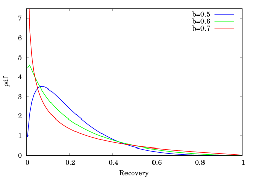
Figure 1: Vasicek distributions with mean 0.2 and width parameter 0.5, 0.6, 0.7.

which has mean $\Phi(a)$ and variance $\Phi_{2}(a,a;b^{2})-\Phi(a)^{2}$. (Here $\Phi_{2}(x,y;\rho)$ denotes as usual the cumulative bivariate Normal distribution.) For small $b$ the standard deviation is roughly $\phi(a)b$, which follows from the tetrachoric series expansion of $\Phi_{2}$. This enables the distribution to be parametrised in terms of understandable numbers. Notice also that, one can easily model correlated recovery rates of several issuers, if desired, just by correlating their $Z$-variables through a multivariate Normal. Figure 1 shows the density for mean $20\%$ ($a=-0.842$) and three different values of the width parameter $b$ (0.5,0.6,0.7).

The payoffs of a recovery swap (or lock), call, and put are, respectively, $\Re-K$, $(\Re-K)^{+}$ and $(K-\Re)^{+}$, at expiry, where $K$ is the recovery strike. There is no payment if no default occurs. Using the result

$$\mathbf{E}\!\left[\Phi\!\left(\frac{a+bZ}{\sqrt{1-b^{2}}}\right)\mathbf{1}(Z>\xi)\right]=\Phi_{2}(-\xi,a;b)$$

we can obtain the call and put payoffs with strike $u$ as

$$\mathbf{E}[(\Re-u)^{+}] = \Phi_{2}(a,c;b)-\Phi(c)u$$

$$\mathbf{E}[(u-\Re)^{+}] = \Phi(-c)u-\Phi_{2}(a,-c;-b)$$

with $c=\big{(}a-\Phi^{-1}(u)\sqrt{1-b^{2}}\big{)}/b$. That put-call parity is satisfied is evident from elementary symmetries in $\Phi_{2}$.

The option values $C_{\pm}(\Re;u)$ are these expected payoffs multiplied by the difference between the risky and riskfree discount factors (i.e. $B(t_{E})-B^{*}(t_{E})$), because the cashflow occurs at time $t_{E}$ and is contingent upon default before option expiry. The recovery swap PV is obviously the difference between the strike and market recovery level, multiplied by the same factor.

In practice one obviously has to estimate the two parameters $a$ and $b$. Recovery locks do trade so there is some guide from the market as to where recovery is likely to be, but there is no information about uncertainty in recovery. As an example, take the defaults in CDX.HY9 in 2008-09. The average recovery was 17.5% but the dispersion was very wide: the highest was Tembec with 83%, there were a couple at supposedly investment-grade levels (Quebecor 41.25%, Lear 38.4%), but the lowest were almost zero (Tribune 1.5%, Idearc 1.75%, Charter 2.375%, Visteon 3%, Abitibi 3.25%, RHD 4.875%). Thus without any knowledge of the credit one should probably use a high dispersion parameter ($b\sim 0.75$ to fit these points). Of course, there is generally less uncertainty in the market over a particular traded credit, particularly at short horizon, and then the $b$ parameter is selected so as to represent the analysts’ uncertainty.

One might ask whether it is necessary to ‘correlate recovery with default’. First one has to ask what this means. Importantly, the random variable $Z$ is only observed when default occurs, so one only wants its distribution conditional on default: in any other state of the world its value is irrelevant. Its distribution may be time-dependent (so that one has to use a different $a,b$ for different option maturities)—but use of different parameters for different maturities, most notably of course the Black-Scholes volatility, is standard practice.

For multivariate models, the question of correlation takes on a different form, and this is not relevant to the pricing of single-name options. One obviously wishes to correlate default events and there is evidence that when default rates en bloc are higher, recoveries are lower [5, 6]. Incidentally the incorporation of this effect is also valuable in modelling of CDO tranches as it is a convenient device for pushing losses up into the senior tranches, a perennial difficulty for tranche modellers. Now, suppose that at a particular horizon we are to correlate defaults and recoveries for many credits. We want to ensure that we can consistently model correlated defaults and recoveries, having specified that the distribution of recovery (conditional, as said before, on default) is Vasicek. It turns out that this is possible without restricting the dependence structure, and this is discussed in the Appendix.

2.7 Example

We consider option pricing with the following parameters: vol 100%, recovery 20%, pricing date 09-Nov-09, option expiry 20-Mar-10, swap maturity 20-Dec-14. For no-knockout options we need the recovery rate volatility, and this is given via the ‘$b$’ parameter which we take to be 0.6.

Figure 2 is for spot=500bp (forward-starting RPV01 3.723). The leftmost points on the graph are the payer and receiver premiums for all-running strike (500bp), which can be checked against the standard Black-Scholes price. The other points show the prices of options in which the strike is quoted partly upfront: the conversion is that 100bp running corresponds to 3.72% upfront, and the all-upfront strike is 18.6%. As expected the option prices decrease as the proportion of the upfront increases. The KO payer should be 35bp cheaper for all-upfront strike than for all-running, and the receiver about 100bp cheaper. The NKO payer options are obviously more expensive than their KO counterparts, by an amount that decreases as the upfront part is raised. For the receiver the embedded recovery call option is too far out of the money to have noticeable value.

3 Index options

Index options are best treated as a separate asset class from single-name options because a literal model of an index option would require a model of correlated spreads and defaults between all the issuers. Such an exercise (bottom-up approach) is not necessarily a bad idea, particularly if one wants to consider where the market for index options ‘should’ be trading. While this is potentially useful for strategising it is probably not useful for pricing. As likely as not, it will fail to match the market and then one has to work out which of the many parameters to adjust. By convention they trade no-knockout, so that exercise is into the ‘original’ index without removing any credits that have defaulted in the life of the option, and this is the case that we analyse here. As pointed out by O’Kane [10], the decision to exercise or not depends on the accrued loss in the pool, as well as the current spread and RPV01, so it is not possible to simply add the front-end protection to the payer price in the way that is done for single-name options.

On exercise of an index payer, the following payments are made:

• Option buyer receives par minus recovery on all defaulted names since the option was struck;

• Option buyer effectively exercises into an index contract, at the prevailing market spread, on the remaining notional, i.e. the original notional multiplied by the proportion of names that are still undefaulted (this is usually cash-settled though);

• Option buyer pays a cash amount equal to the strike spread minus the index coupon, multiplied by a PV01 defined by convention as $\widetilde{\Pi}_{t_{E}}(s_{K};t_{E},T)$, that is, the RPV01 assuming a flat curve at the strike spread (not the prevailing market spread, which would be undefined in the armageddon event), on the full notional.

Symbolically, we have that the value of an index payer is

$$C^{\textrm{+idx}}=\mathbf{E}_{t}\left[\frac{\mathfrak{B}_{t}}{\mathfrak{B}_{t_{E}}}\left(L_{t_{E}}+\frac{N_{t_{E}}}{N_{00}}(s_{t_{E}}-c)\widetilde{\Pi}_{t_{E}}(s_{t_{E}};t_{E},T)-\frac{N_{0}}{N_{00}}(s_{K}-c)\widetilde{\Pi}_{t_{E}}(s_{K};t_{E},T)\right)^{+}\right]$$

Here $\widetilde{\Pi}_{t}(s;T_{1},T_{2})$ is the ‘flat-hazard-rate’ PV01 calculation alluded to above. It is simply a formal calculation to get from a spread to an upfront for use in settlement, and does not, for example, depend on the number of defaults in the index (though it does depend on an assumed recovery rate which is fixed by market convention), and nor is it a tradable asset as such. It is worth noting that the quantity

$$\frac{N}{N_{00}}(s-c)\widetilde{\Pi}(s;t,T)$$

is obtainable immediately from the Bloomberg CDSW screen, because it is the upfront (settlement amount) of an index CDS contract; so a market participant can easily calculate it. It is therefore consistent with CDS index option pricing methods. The quantity $L_{t}$ is the accrued loss through defaults from time 0 to time $t$ and $N_{t}$ is the number of survived names at time $t$. (Notice, by the way, that the formula for $L_{t}$ after Eq.(42) in [12] is incorrect, as the recoveries of the defaulted names may be different.) The option is assumed to have been struck at time 0, and $N_{00}$ denotes the number of names in the original index: for example we might have $N_{00}=125$, $N_{0}=124$ and $N_{t}=122$, meaning that the index originally had 125 names, one default occurred, then the option was written, then another two occurred, and now it is time to value the optionIt is also to be understood that $s_{t}$ is the spread of the version of the index current at time $t$ (i.e. with names that defaulted before time $t$ removed; $L_{t}$ keeps track of the defaulted ones).

For calculating the ISDA RPV01 $\widetilde{\Pi}$ the following approximation is helpful. With $\lambda=\widehat{s}/(1-\Re)$, and $Q(T)$ the survival probability,

$$\widetilde{\Pi}^{(}T) = \int_{0}^{T}B^{\circ}(t)Q(t)\,dt$$ (7)

$$\approx \frac{1}{T}\int_{0}^{T}B^{\circ}(t)\,dt\int_{0}^{T}Q(t)\,dt$$

$$= \Pi^{\circ}(T)\frac{1-e^{-\lambda T}}{\lambda T}\mbox{ if }Q(t)=e^{-\lambda t}$$

$$\approx \frac{\Pi^{\circ}(T)}{1+\frac{1}{2}\lambda T+\frac{1}{12}(\lambda T)^{2}}$$ (8)

so that the RPV01 is obtained by multiplying the swap (riskfree) PV01, $\Pi^{\circ}$, by a factor that reduces it by roughly the right amount. The last line follows from the expansion of $\frac{x}{1-e^{-x}}$ in a Taylor series using the Bernoulli numbers.

A minor point worth ironing out is what happens when the strike spread is made arbitrarily high. According to O’Kane, the payer option should become worthless in that limit, on the grounds that one is paying an ‘infinite spread’ on exercise, whereas the simple procedure of taking a knockout payer Black’76 style and adding on the front-end protection causes the payer value to tend to the value of the front-end protection. In fact, both are wrong, because the exercise premium does not tend to infinity: its limit is, as can be easily verified,

$$\lim_{s_{K}\to\infty}(s_{K}-c)\widetilde{\Pi}_{t}(s_{K};t_{E},T)=1-\Re$$

where $\Re$ is the index recovery used in the RPV01 calculation. The ‘infinite spread’ argument is a fairly common error, made by those who forget that the coupon is fixed, i.e. that the CDS is not a par instrument.

The forward spread $s_{F}$ is defined to be the fair spread for paying CDS premium and receiving protection. If we follow the usual argument that buying a CDS forward and selling today should have zero PV, then the forward spread is given by the solution to

$$(s_{F}-c)\widetilde{\Pi}_{0}(s_{F};t_{E},T)=(s_{0}-c)\widetilde{\Pi}_{0}(s_{0};0,T)+c\Pi^{*}_{0}(0,t_{E})$$ (9)

with $\Pi^{*}$ the true risky PV01(). This is approximately

$$s_{F}\approx s_{0}\frac{\widetilde{\Pi}_{0}(s_{0};0,T)}{\widetilde{\Pi}_{0}(s_{0};t_{E},T)}.$$

The forward is therefore higher than the strike. The main reason for this is not that the curve is upward-sloping, but that it is a no-knockout forward: by buying forward protection today for the period $[t_{E},T]$ one is not giving up the payout arising from defaults in the time interval $[0,t_{E}]$. In essence one is buying the same protection but paying for it over a shorter period of time, necessitating a higher running premium.

We want to explicitly model the option as one on the difference between two PV’s $X$ and $Y$ say, i.e. the default-PV of the underlying swap and the PV of the coupon leg that would be exercised into at the prescribed strike, change numeraire to $Y$ and then use Black’76. Note that in the context of the single names we avoided this approach for the part-upfront options, because of inconsistency with the all-running case: with the index options there is only one product to model, so we can deal with that as the de facto standard.

However, we can only use this construction if $X$ and $Y$ are positive a.s. Therefore we have to be a little careful in grouping the terms, and the following construction achieves this in an intuitive way:

$$X_{t} = L_{t}+\frac{N_{t}}{N_{00}}(s_{t}-c)\widetilde{\Pi}_{t}(s_{t};t,T)+\frac{cN_{0}}{N_{00}}A_{t}$$ (10)

$$Y_{t} = \frac{N_{0}}{N_{00}}\Big{(}(s_{K}-c)\widetilde{\Pi}_{t}(s_{K};t_{E},T)+cA_{t}\Big{)}$$ (11)

$$A_{t} = \widetilde{\Pi}_{t}(0;t,T)=\Pi^{\circ}(t,T)$$ (12)

The extra term $A_{t}$ is explained as follows. The expression $X_{t}$ is the PV at time $t$ of a long index protection trade entered into at time 0 for an investor who is assumed to own a riskfree annuity to pay the cost of carry during the life of the trade, thereby making the trade fully-funded. This is because the first term in (10) is the accrued payout from defaults, the second is the PV of the remaining index protection, and the third ($A_{t}$) is the PV of the remaining cashflows of the annuity. It is easy to see that $X_{t}>0$ a.s., because the first term is nonnegative and $A_{t}$ exceeds the negative part of the second term in $X_{t}$. In fact $X_{t}$ approaches $0$ in the situation where $N_{t}=N_{0}$ (so $L_{t}=0$) and $s_{t}\to 0$. It is also clear that $Y_{t}>\frac{N_{0}}{N_{00}}s_{K}\widetilde{\Pi}_{t}(s_{K};t_{E},T)$ a.s. by similar reasoning. Notice that all the correction terms result from the presence of the index coupon. Finally, $X_{t}$ and $Y_{t}$ are well-defined even in the armageddon event, for although $s_{t}$ and hence $\widetilde{\Pi}_{t}(s_{t};t,T)$ are no longer defined, the term that references them is being multiplied by $N_{t}/N_{00}$ which is zero and so it vanishes.

We need the discounted expectations of $X_{t_{E}}$ and $Y_{t_{E}}$ at time $t$, i.e.

$$\tilde{X}_{t}:=\mathbf{E}_{t}[X_{t_{E}}\mathfrak{B}_{t}/\mathfrak{B}_{t_{E}}],\qquad\tilde{Y}_{t}:=\mathbf{E}_{t}[Y_{t_{E}}\mathfrak{B}_{t}/\mathfrak{B}_{t_{E}}].$$

By construction $X_{t}$ is the PV of a sum of tradable assets, so

$$\tilde{X_{t}}=X_{t}.$$

At initiation one has simply

$$\tilde{X}_{0}=\frac{N_{0}}{N_{00}}\Big{(}s_{0}\widetilde{\Pi}_{0}(s_{0};0,T)+c\big{(}\widetilde{\Pi}_{0}(0;t_{E},T)\big{)}\Big{)}-c\mathbf{E}_{0}\Big{[}\frac{N_{t_{E}}}{N_{00}}\widetilde{\Pi}_{t_{E}}(s_{t_{E}};t_{E},T)\frac{\mathfrak{B}_{0}}{\mathfrak{B}_{t_{E}}}\Big{]}.$$

The last term can be approximated by $-c\frac{N_{0}}{N_{00}}\widetilde{\Pi}_{0}(s_{0};t_{E},T)$, which leaves us with:

$$\tilde{X}_{0}\approx\frac{N_{0}}{N_{00}}\Big{(}s_{0}\widetilde{\Pi}_{0}(s_{0};0,T)+c\big{(}\widetilde{\Pi}_{0}(0;t_{E},T)-\widetilde{\Pi}_{0}(s_{0};t_{E},T)\big{)}\Big{)}.$$

Similarly, $Y_{t}$ is a tradable asset and at initiation one has:

$$\tilde{Y}_{0}=\frac{N_{0}}{N_{00}}\Big{(}s_{K}\widetilde{\Pi}_{0}(s_{K};t_{E},T)+c\big{(}\widetilde{\Pi}_{0}(0;t_{E},T)-\widetilde{\Pi}_{0}(s_{K};t_{E},T)\big{)}\Big{)}$$

We can now use the Black formula for valuing the option to exchange one asset for another. The final result is then:

$$C^{+\textrm{idx}}_{t} = \tilde{X}_{t}\Phi(d_{+})-\tilde{Y}_{t}\Phi(d_{-}),$$ (13)

$$C^{-\textrm{idx}}_{t} = \tilde{Y}_{t}\Phi(-d_{-})-\tilde{X}_{t}\Phi(-d_{+}),$$ (14)

$$\tilde{X}_{t}=\mbox{Eq.}(\ref{eq:Xt1});\quad\tilde{Y}_{t}=\mbox{Eq.}(\ref{eq:Yt1});\quad d_{\pm}=\frac{\ln(\tilde{X}_{t}/\tilde{Y}_{t})\pm\frac{1}{2}\sigma^{2}(t_{E}-t)}{\sigma\sqrt{t_{E}-t}}$$ (15)

where $\sigma$ is the volatility of $X/Y$. The delta is given, as usual, by $\Phi(d_{+})$. Notice that for at-the-money-forward options, by put-call parity, we have

$$C^{+\textrm{idx}}_{0}-C^{-\textrm{idx}}_{0}=\tilde{X}_{0}-\tilde{Y}_{0}=\frac{N_{0}}{N_{00}}\big{(}s_{0}\widetilde{\Pi}_{0}(s_{0};0,T)-s_{F}\widetilde{\Pi}_{0}(s_{F};t_{E},T)\big{)}\approx 0.$$

We have deliberately left the relevant quantities as PV’s rather than converting them back to spreads. One could try to write $X_{t}$ and $Y_{t}$ in terms of a corrected forward spread and a corrected strike (the corrections being for the coupon effect and the accrued loss), viz:

$$\tilde{X}_{t} = s^{*}_{F,t}\widetilde{\Pi}_{t}(s_{t};t,T),\qquad s^{*}_{F,t}=\frac{N_{t}}{N_{00}}s_{0}+\frac{L_{t}}{\widetilde{\Pi}_{t}(s_{t};t,T)}+c(\ldots)$$

$$\tilde{Y}_{t} = s_{K}^{*}\widetilde{\Pi}_{t}(s_{K};t_{E},T),\qquad s_{K}^{*}=s_{K}+c(\ldots).$$

But this does not seem to achieve anything useful: the PV01s are different, and it also unearths the previously-buried problem of what happens in the armageddon event ($\tilde{X}_{t}$ is well-defined but $s^{*}_{F,t}$ is not). Notice incidentally that some of the adjusted forward corrections in the literature can result in a negative adjusted forward and/or strike spread, in the admittedly unlikely situation of the strike being very low. The construction used here renders this impossible.

In some respects the formulation would be neater if the annuity being added to $X_{t}$ were risky rather than riskfree: in other words, one that paid the coupon only on the undefaulted names. The PV of such an instrument would then be $\Pi^{*}(t,T)$ which is slightly lower than $\Pi^{\circ}(t,T)$, and it is still enough to render $X_{t}>0$. Indeed, if we approximate the true risky PV01 $\Pi^{*}(t,T)$ by the ISDA one, then we have

$$\tilde{X}_{0}\approx\frac{N_{0}}{N_{00}}s_{0}\widetilde{\Pi}_{0}(s_{0};0,T)$$

and

$$\tilde{Y}_{0}\approx\frac{N_{0}}{N_{00}}\Big{(}s_{K}\widetilde{\Pi}_{0}(s_{K};t_{E},T)+c\big{(}\widetilde{\Pi}_{0}(s_{0};t_{E},T)-\widetilde{\Pi}_{0}(s_{K};t_{E},T)\big{)}\Big{)}.$$

But there is a minor snag: if $s_{K}$ is low enough then $Y$ can become negative. In practice this is probably not worth worrying about.

Incidentally the CDX.HY (high-yield) index is quoted as a bond price, but still trades as a swap. (For example, a price of 97.625 means that a buyer of index protection pays $2.375$% upfront plus 500bp running.) It is convenient to work with the prevailing upfront $U_{t}$, which pertains to the version of the index at time $t$ (as we said earlier: with names that defaulted before time $t$ removed, because $L_{t}$ keeps track of the defaulted ones) and an upfront strike $u_{K}$; these will be negative if the associated bond price exceeds 100. The index payer, which is usually referred to as a put, has value

$$\mathbf{E}_{t}\left[\displaystyle\frac{\mathfrak{B}_{t}}{\mathfrak{B}_{t_{E}}}\left(L_{t_{E}}+\frac{N_{t_{E}}}{N_{00}}U_{t_{E}}-\frac{N_{0}}{N_{00}}u_{K}\right)^{+}\right].$$

Our construction is now the same as before, only simpler:

$$X_{t} = L_{t}+\frac{N_{t}}{N_{00}}U_{t}+\frac{cN_{0}}{N_{00}}A_{t}$$ (16)

$$Y_{t} = \frac{N_{0}}{N_{00}}(u_{K}+cA_{t})$$

and $A_{t}$ as before (12).

To find the forward upfront given prices instead of spreads, one can use the following equation:

$$U_{F}=U_{0}+c\widetilde{\Pi}_{0}(s_{0};0,t_{E})$$

3.1 Example

Table 2 shows the option payer and receiver prices for CDX.IG28 that we computed (initiation and pricing date 06-Jul-17; option expiry 20-Sep-17; index maturity 20-Jun-22; coupon 100bp; spot 61bp; recovery 40%; swap rate 2.05%). The volatilities being used were from a recent dealer run. Table 2 shows the results for CDX.HY28 priced on 13-Jul-17 with coupon 500bp, spot price 107.125, recovery 30% and swap rate 2%. No credit event had taken place, so $\frac{N_{0}}{N_{00}}=1$.

Tables 4 and 4 show the options payer and receiver prices for iTraxx Crossover option series 27 with maturity dates in September and December 2017. The pricing date is 19-Jul-17; index maturity 20-Jun-22; coupon 500bp; spot 240bp; recovery 30%; swap rate 0.75% and $\frac{N_{0}}{N_{00}}=1$.

4 Conclusions

We have shown how to value, in the Black’76 framework, single-name CDS options in which the strike is quoted wholly or partially upfront and shown that the proportion of upfront has a significant impact on price, if consistency with the standard ‘all-running’ case is to be achieved. We have also pointed out that no-knockout single-name options that are quoted wholly or partially upfront contain an embedded recovery option, and given a simple explicit formula for the price. The treatment of index options that we have given here is not revolutionary, but rather is intended to deal with the payout more carefully and intuitively.

5 Appendix

We discuss the correlation of recovery and default in a multivariate setting (see e.g. [16]). This goes well beyond the scope of this paper and is only intended as a brief justification of our previous assertion that the univariate model we have given can be extended to the multivariate case (in infinitely many ways, in fact).

This is most conveniently done with the assistance of a risk-factor, i.e. a random variable $\mathcal{A}$ say (which need not be univariate). Conditionally on $\mathcal{A}$, all recoveries and defaults are completely independent. Let a particular credit have a conditional default probability $p(\mathcal{A})$, so that $\mathbf{E}[p(\mathcal{A})]=\overline{p}$ (the average default probability, in this case obtained from the CDS market). Let $F$ be an arbitrary (cumulative) distribution function, and $\beta$ be a coefficient that will couple the recovery variable $Z$ to the risk-factor $\mathcal{A}$. Define

$$F_{\sharp}(z):=\frac{1}{\overline{p}}\,\mathbf{E}[F(z-\beta\cdot\mathcal{A})p(\mathcal{A})].$$

Then define the conditional distribution of $Z$ on $\mathcal{A}$ to be

$$\mathbf{P}[Z<z\,|\,\mathcal{A}]=F\big{(}F_{\sharp}^{-1}(\Phi(z))-\beta\cdot\mathcal{A}\big{)}.$$

The distribution of $Z$ conditionally on default of the issuer within the horizon $t_{E}$, but unconditionally on $\mathcal{A}$, is

$$\mathbf{P}[Z<z\,|\,\tau<t_{E}]=\frac{1}{\overline{p}}\,\mathbf{E}\big{[}\mathbf{P}[Z<z\,\cap\tau<t_{E}\,|\,\mathcal{A}]\big{]}$$

$$=\frac{1}{\overline{p}}\,\mathbf{E}\left[p(\mathcal{A})F\big{(}F_{\sharp}^{-1}(\Phi(z))-\beta\cdot\mathcal{A}\big{)}\right]=F_{\sharp}\big{(}F_{\sharp}^{-1}(\Phi(z))\big{)}=\Phi(z)$$

which is what we wanted it to be. This procedure of constructing what might be described as ‘additive factor-copulas’ is quite generally applicable and shows that one can always match a given marginal distribution. As stated above, $\beta$ plays the role of a correlation parameter, while the distribution chosen for $F$ is completely arbitrary.

I acknowledge helpful discussions with Philipp Schönbucher, Ismail Iyigunler and the credit quant/trading desks at Credit Suisse, JP Morgan and Deutsche Bank. I also thank Huong Vu for her kind assistance with the CDS index numerics. Email: richard.martin1@imperial.ac.uk

Figure 2: Knockout and no-knockout option prices as a function of the upfront part of the strike; spot 500bp. Payers: $\circ$=KO, $\bullet$=NKO, both on LH axis. Receivers: $\square$=KO, $\blacksquare$=NKO, both on RH axis (they differ by $<0.1$bp). Running part of strike decreases linearly from 500bp to 0bp.

Strike	Vol	Payer	Delta	Receiver	Delta
55	29%	42.6	88%	2.5	12%
57.5	31%	34.2	79%	5.5	21%
60	33%	27.3	68%	9.9	32%
62.5	34%	21.3	58%	15.2	42%
65	36%	17.1	49%	22.3	51%
67.5	38%	13.8	41%	30.3	59%
70	39%	10.8	34%	38.5	66%
72.5	41%	9.0	29%	47.9	71%
75	43%	7.6	24%	57.7	76%
80	46%	5.3	17%	77.7	83%
85	50%	4.2	14%	98.9	86%
90	52%	3.0	10%	119.8	90%

Table 1: CDX.IG28 Option payer and receiver prices

Strike	Vol	Payer	Delta	Receiver	Delta
108.5	22%	236.6	95%	3.7	5%
108	23%	192.5	89%	9.6	11%
107.5	25%	155.3	79%	22.4	21%
107	27%	124.8	69%	41.9	31%
106.5	29%	100.7	59%	67.8	41%
106	31%	82.0	50%	99.0	50%
105.5	33%	67.6	42%	134.7	58%
105	35%	56.5	36%	173.6	64%
104	37%	36.8	25%	253.9	75%
103	40%	26.4	18%	343.5	82%
102	42%	18.3	13%	435.4	87%

Table 2: CDX.HY28 Option payer and receiver prices

Strike	Vol	Payer	Delta	Receiver	Delta
200	31.1%	240.9	95%	3.8	5%
212.5	31.4%	185.9	88%	10.5	12%
225	32.4%	138.8	77%	24.4	23%
250	35.1%	72.6	52%	78.6	48%
275	38.6%	38.4	31%	162.9	69%
300	44.6%	25.3	20%	266.2	80%
325	48.9%	16.9	14%	372.3	86%
350	52.8%	12.0	10%	479.9	90%
375	56.8%	9.3	7%	587.7	93%
400	60.4%	7.4	6%	694.5	94%
425	63.3%	5.9	5%	799.8	95%
450	66.1%	4.9	4%	903.7	96%

Table 3: iTraxx.XO27 (expiring 20-Sep-17)

Strike	Vol	Payer	Delta	Receiver	Delta
200	33.5%	299.5	90%	15.1	10%
225	33.8%	210.7	78%	40.6	22%
250	35.0%	144.6	62%	86.6	38%
275	37.4%	101.9	48%	154.2	52%
300	41.0%	77.8	38%	238.3	62%
325	43.8%	60.4	30%	327.2	70%
350	46.6%	48.9	25%	420.2	75%
375	49.3%	41.0	21%	514.8	79%
400	51.7%	35.0	17%	609.5	83%
425	53.7%	30.0	15%	703.4	85%
450	54.7%	24.6	13%	795.1	87%
475	55.7%	20.5	11%	886.3	89%

Table 4: iTraxx.XO27 (expiring 20-Dec-17)

References

- [1] H. Ben-Ameur, D. Brigo, and E. Errais. A dynamic programming approach for pricing CDS and CDS options. www.defaultrisk.com, 2006.
- [2] T. Björk. Arbitrage Theory in Continuous Time. Oxford University Press, 1998.
- [3] D. Brigo and N. El-Bachir. An exact formula for default swaptions pricing in the the SSRJD stochastic intensity model. www.defaultrisk.com, 2008.
- [4] D. Brigo and M. Morini. Last option before the armageddon. RISK, 22(9):118–123, 2009.
- [5] M. Bruche and C. González-Aguado. Recovery rates, default probabilities, and the credit cycle. www.defaultrisk.com, 2008.
- [6] P. Dobranszky. Joint modelling of CDS and LCDS spreads with correlated default and prepayment intensities and with stochastic recovery rate. www.defaultrisk.com, 2008.
- [7] S. Doctor and J. Goulden. An introduction to credit options and credit index volatility. JP Morgan Credit Derivatives Research, March, 2007.
- [8] A. Herbertsson. CDS index options in Markov chain models. Technical report, Dept. of Economics, Univ. of Gothenburg, 2019. Working Paper No.748.
- [9] J. Hull and A. White. Valuing credit default swap options. J. Derivatives, 10(3):40–50, 2003.
- [10] D. O’Kane. Valuing single-name and multi-name credit derivatives. Wiley, 2008.
- [11] C. Pedersen. Valuation of portfolio credit default swaptions. Lehman Brothers Quantitative Credit Research, November, 2003.
- [12] M. Rutkowski and A. Armstrong. Valuation of credit default swaptions and credit default index swaptions. Technical report, School of Mathematics and Statistics, Economics & Law, Univ. of New South Wales, 2008.
- [13] P. Schönbucher. Credit Derivatives Pricing Models. Wiley, 2003.
- [14] P. Schönbucher. A measure of survival. RISK, 17(8):79–85, 2004.
- [15] E. Sveder and E. Johansson. Pricing credit default index swaptions. Technical report, School of Business, Economics & Law, Univ. of Gothenburg, 2015.
- [16] D. Tasche. The single risk factor approach to capital charges in case of correlated loss given default rates. www.defaultrisk.com, 2004.