Unobservable Planar Bimodal Linear Systems: Miniversal Deformations, Controllability and Stabilization

Abstract

We consider the set of bimodal linear systems consisting of two linear dynamics acting on each side of a given hyperplane, assuming continuity along the separating hyperplane. Focusing on the unobservable planar ones, we obtain a simple explicit characterization of controllability. Moreover, we apply the canonical forms of these systems depending on two state variables to obtain explicitly miniversal deformations, to illustrate bifurcation diagrams and to prove that the unobservable controllable systems are stabilizable.

1 Introduction

Piecewise linear systems have attracted the interest of the researchers in recent years by their wide range of applications, as well as by the possible theoretical approaches. In both directions, the non-generic case of unobservable systems presents interesting particularities. They appear in a natural way in parameterized families, bifurcations,…, and special theoretical tools are needed to study their properties.

In this paper, we consider the set of bimodal linear systems consisting of two linear dynamics acting on each side of a given hyperplane, assuming continuity along the separating hyperplane. In the space of triples of matrices defining those systems, we consider the natural equivalence relation defined by changes of bases in the state space which preserves the hyperplanes parallel to the separating hyperplane. The fact that this equivalence relation can be viewed as the one induced by the action of a Lie group allows to apply Arnold’s techniques concerning versal deformations, stratification, etc.

Canonical forms, representative for each equivalence class, are a basic tool in order to simplify the computations, because instead of the given matrices their canonical forms can be used. More concretely, we present an explicit expression of the canonical form of a given triple of matrices when the number of state variables is two or three, which are the most commonly found in applications (see for example [3], [4], [5], [6], [9]). We use these canonical forms to obtain explicitly miniversal deformations and to illustrate local bifurcation diagrams always focusing on the unobservable case.

Secondly, we obtain a simple explicit characterization of the controllability of a planar bimodal system, starting on the implicit one in [2]. Indeed, we prove that for $n=2$ one of the conditions there can be avoided (Corollary 9), and the other one can be reformulated in a very simple way (Proposition 8).

Moreover, in [2] one asks if controllable bimodal linear systems can be stabilized by means of a feedback (the same for both subsystems), generalizing the well-known result for a single system. Here the reformulation of controllability (Corollary 10) and the above canonical forms are used to prove that this is true in the unobservable planar case (Theorem 11).

The structure of the paper is as follows. In Section 2 we provide the canonical forms obtained for a bimodal linear system in the cases where the number of state variables is two, and recall the dimensions of the orbits and the strata. As an application, in Section 3 we compute miniversal deformations and apply them to obtain local bifurcation diagrams. Section 4 is devoted to obtain a simple explicit characterization of the controllability and to prove that then the system is stabilizable by feedback.

Throughout the paper, $\mathbb{R}$ will denote the set of real numbers, $M_{n\times m}(\mathbb{R})$ the set of matrices having $n$ rows and $m$ columns and entries in $\mathbb{R}$ (in the case where $n=m$, we will simply write $M_{n}(\mathbb{R})$) and $Gl_{n}(\mathbb{R})$ the group of non-singular matrices in $M_{n}(\mathbb{R})$. Finally, we will denote by $e_{1},\dots,e_{n}$ the natural basis of the Euclidean space ${\mathbb{R}}^{n}$.

2 Canonical Forms

Let us consider a bimodal linear dynamical system given by

$$\begin{cases}\dot{\boldsymbol{x}}(t)=A_{1}\boldsymbol{x}(t)+B_{1},\\ \boldsymbol{y}(t)=C\boldsymbol{x}(t),\end{cases}\ \text{ if }\;\boldsymbol{y}(t)\leq 0,\quad\begin{cases}\dot{\boldsymbol{x}}(t)=A_{2}\boldsymbol{x}(t)+B_{2},\\ \boldsymbol{y}(t)=C\boldsymbol{x}(t),\end{cases}\ \text{ if }\;\boldsymbol{y}(t)\geq 0$$

where $A_{1},A_{2}\in M_{n}(\mathbb{R})$; $B_{1},B_{2}\in M_{n\times 1}(\mathbb{R})$; $C\in M_{1\times n}(\mathbb{R})$. Let us assume that the dynamics is continuous along the separating hyperplane $H=\{\boldsymbol{x}\in\mathbb{R}^{n}:C\boldsymbol{x}=0\}$. For simplicity, we will consider that $C=(1\;0\ldots 0)\in M_{1\times n}({{\mathbb{R}}})$. Hence $H=\{\boldsymbol{x}\in\mathbb{R}^{n}:x_{1}=0\}$ and continuity along $H$ is equivalent to:

$$B_{2}=B_{1},\qquad A_{2}e_{i}=A_{1}e_{i},\quad 2\leq i\leq n.$$

We will write from now on $B=B_{1}=B_{2}$.

Definition 1

In the above conditions, we say that the triple of matrices $(A_{1},A_{2},B)$ defines a bimodal piecewise linear system. Throughout the paper, $\mathcal{X}$ will denote the set of these triples

$$\mathcal{X}=\left\{(A_{1},A_{2},B)\in M_{n}(\mathbb{R})\times M_{n}(\mathbb{R})\times M_{n\times 1}(\mathbb{R})\left|\;A_{2}e_{i}=A_{1}e_{i},\>2\leq i\leq n\right.\right\}$$

which is obviously a ($n^{2}+2n$)-differentiable manifold.

The system is called observable if

$$\mathop{\rm rank}\nolimits\left(\begin{array}[]{c}C\\ CA_{i}\\ \cdots\\ CA_{i}^{n-1}\end{array}\right)=n,\quad i=1,2.$$

The basis changes in the state variables space preserving the hyperplanes $x_{1}(t)=k$ will be called admissible basis changes. Thus, they are basis changes given by a matrix $S\in Gl_{n}(\mathbb{R})$,

$$S=\left(\begin{array}[]{cc}1&0\\ U&T\end{array}\right),\quad T\in Gl_{n-1}(\mathbb{R}).$$

We consider the equivalence relation in the set of triples of matrices $\mathcal{X}$ which corresponds to admissible basis changes:

Definition 2

We write

$$\mathcal{S}:=\left\{S\in\,Gl_{n}(\mathbb{R})\left|\,S=\left(\begin{array}[]{cc}1&0\\ U&T\end{array}\right),\;T\in Gl_{n-1}({\mathbb{R}})\right.\right\}.$$

Then, $(A_{1},A_{2},B),(A^{\prime}_{1},A^{\prime}_{2},B^{\prime})\in\mathcal{X}$ are said to be equivalent if there exists a matrix $S\in{\cal S}$ (representing an admissible basis change) such that $(A^{\prime}_{1},A^{\prime}_{2},B^{\prime})=(S^{-1}A_{1}S,S^{-1}A_{2}S,S^{-1}B)$.

Notice that the matrix $C$ is not involved in this definition since $CS=C$ for any $S\in{\cal S}$.

We remark that equivalence classes are actually the orbits with regard to the action of the Lie group ${\cal S}$ on the differentiable manifold ${\cal X}$,

$$\begin{array}[]{rl}\alpha:{\cal S}\times{\cal X}&\longrightarrow{\cal X}\end{array}$$

defined by

$$\alpha(S,{\cal X})=(S^{-1}A_{1}S,S^{-1}A_{2}S,S^{-1}B)$$

Given any triple of matrices $(A_{1},A_{2},B)\in{\cal X}$, we will denote by ${\cal O}(A_{1},A_{2},B)$ its orbit (or equivalence class).

As an application of the Closed Orbit Lemma (see [10]), we deduce that equivalence classes are differentiable manifolds. Namely, any equivalence class is a locally closed differentiable submanifold of ${\cal X}$ and its boundary is a union of equivalence classes or orbits of strictly lower dimension. In particular, equivalence classes or orbits of minimal dimension are closed.

In this section we summarize the results in the previous works [7] and [8] which will be used in the sequel. The first goal is obtaining for each triple $(A_{1},A_{2},B)$ a canonical reduced form which characterizes its equivalence class. In http://www.ma1.upc.edu/$\sim$joanr/html/cfbpwls.html the reader can find a MAPLE program which allows to obtain the canonical form of a triple $(A_{1},A_{2},B)$ for the cases $n=2$ and $n=3$, which are the most commonly systems found in practice. Furthermore, one obtains an admissible basis change $S\in{\cal S}$ which transforms the initial triple $(A_{1},A_{2},B)$ into its canonical form.

When listing canonical forms, it is necessary that the coefficients appearing in them as well as the conditions used to distinguish the different types do not depend on the admissible basis which one considers, that is to say, they are preserved under admissible basis changes $S\in{\cal S}$. It is well-known that $\mathop{\rm tr}\nolimits A_{1}$, $\mathop{\rm tr}\nolimits A_{2}$, $\det A_{1}$, $\det A_{2}$ are invariant under any basis change $S\in Gl_{n}(\mathbb{R})$. We focus on the additional invariants when only admissible basis changes $S\in\mathcal{S}$ are considered.

Definition 3

A real number (respectively a property) associated to a triple $(A_{1},A_{2},B)$ is called $\mathcal{S}$-invariant if it is preserved by admissible basis changes, that is to say, it has the same value (respectively it is also true) for any other triple $(A^{\prime}_{1},A^{\prime}_{2},B^{\prime})$ $\mathcal{S}$-equivalent to the given one.

For example, it is obvious that:

Proposition 1

They are $\mathcal{S}$-invariant:

1. The top coefficient $b_{1}$ in $B$ ($b_{1}=CB$).

2. The matrix $C$.

3. The condition of $(A_{1},A_{2},B)$ being observable.

Next proposition details the remainder $\mathcal{S}$-invariants that we will use for $n=2$. In order to that, we define:

Definition 4

Given a triple

$$A_{1}=\left(\begin{array}[]{cc}a_{1}&a_{3}\\ a_{2}&a_{4}\end{array}\right),A_{2}=\left(\begin{array}[]{cc}\gamma_{1}&a_{3}\\ \gamma_{2}&a_{4}\end{array}\right),B=\left(\begin{array}[]{c}b_{1}\\ b_{2}\end{array}\right)$$

we write:

$$\begin{array}[]{rl}&\Delta_{0}=\det\left(\begin{array}[]{cc}a_{3}&b_{1}\\ a_{4}&b_{2}\end{array}\right)=a_{3}b_{2}-a_{4}b_{1}\\ &\Delta_{12}=a_{2}(a_{4}-\gamma_{1})-\gamma_{2}(a_{4}-a_{1})\\ &\Delta_{1}=b_{1}a_{2}+(a_{4}-a_{1})b_{2}\\ &\Delta_{2}=b_{1}\gamma_{2}+(a_{4}-\gamma_{1})b_{2}\end{array}$$

Lemma 2

The above triple is unobservable if and only if $a_{3}=0$. In this case we have:

1. $\det\left(\left(\begin{array}[]{c}a_{1}-\gamma_{1}\\ a_{2}-\gamma_{2}\end{array}\right)\left|A_{i}\left(\begin{array}[]{c}a_{1}-\gamma_{1}\\ a_{2}-\gamma_{2}\end{array}\right)\right.\right)=(a_{1}-\gamma_{1})\Delta_{12}$, $i=1,2$
   $\det\left(\begin{array}[]{c|c}B&A_{i}B\end{array}\right)=b_{1}\Delta_{i}$, $i=1,2$

2. The action of $S\in\mathcal{S}$ transforms $\Delta_{1}$, $\Delta_{2}$, $\Delta_{12}$ respectively into:

   $$\frac{1}{\det S}\Delta_{1},\quad\frac{1}{\det S}\Delta_{2},\quad\frac{1}{\det S}\Delta_{12}$$

   In particular, it is $\mathcal{S}$-invariant the sign (positive, negative or zero):

   $$\mathop{\rm sign}\nolimits(\Delta_{1}\Delta_{2})$$

Proof. Clearly,

$$\left(\begin{array}[]{c}C\\ CA_{1}\end{array}\right)=\left(\begin{array}[]{cc}1&0\\ a_{1}&a_{3}\end{array}\right),\quad\left(\begin{array}[]{c}C\\ CA_{2}\end{array}\right)=\left(\begin{array}[]{cc}1&0\\ \gamma_{1}&a_{3}\end{array}\right)$$ (1)

do not have maximal rank when $a_{3}=0$. Then:

1. It is a straightforward computation.

2. If $a_{3}=0$, then $a_{1}$ and $\gamma_{1}$ are eigenvalues of $A_{1}$ and $A_{2}$.
   The action of $S$ transforms the matrices in (1) into their left product by $S^{-1}$.

 

Proposition 3

With the above notation, the following table summarizes some $\mathcal{S}$-invariant numbers and properties, as well as the hypotheses for each one:

numbers properties (1) $\Delta_{0}$ $a_{3}=0$ (2) $b_{1}=0$ $b_{2}=0$ (3) $a_{3}=0$ $a_{1},\gamma_{1},a_{4}$ $\Delta_{12}=0,\Delta_{1}=0,\Delta_{2}=0$ (3’) $a_{3}=0,\Delta_{12}\neq 0$ $\Delta_{1}/\Delta_{12},\Delta_{2}/\Delta_{12}$ (4) $a_{3}=0,a_{1}=a_{4}$ $a_{2}=0$ (4’) $a_{3}=0,\gamma_{1}=a_{4}$ $\gamma_{2}=0$ (5) $b_{1}=0,a_{3}=0,a_{1}=a_{4}$ $b_{2}/a_{2}$ (5’) $b_{1}=0,a_{3}=0,\gamma_{1}=a_{4}$ $b_{2}/\gamma_{2}$

Proof.

1. The $\mathcal{S}$-action on $A_{1}$ and $B$ can be formulated as:

   $$S^{-1}(A_{1},B)\left(\begin{array}[]{c|c}S&0\\ \hline\cr 0&1\end{array}\right).$$

   For $n=2$, one has

   $$\left(\begin{array}[]{cc}1&0\\ u&t\end{array}\right)^{-1}\left(\begin{array}[]{ccc}a_{1}&a_{3}&b_{1}\\ a_{2}&a_{4}&b_{2}\end{array}\right)\left(\begin{array}[]{ccc}1&0&0\\ u&t&0\\ 0&0&1\end{array}\right)=\left(\left.\begin{array}[]{c}{\ast}\\ {\ast}\end{array}\right|\left(\begin{array}[]{cc}1&0\\ u&t\end{array}\right)^{-1}\left(\begin{array}[]{cc}a_{3}&b_{1}\\ a_{4}&b_{2}\end{array}\right)\left(\begin{array}[]{cc}t&0\\ 0&1\end{array}\right)\right).$$

   Therefore, $\Delta_{0}$ is $\mathcal{S}$-invariant:

   $$\det\left(\left(\begin{array}[]{cc}1&0\\ u&t\end{array}\right)^{-1}\left(\begin{array}[]{cc}a_{3}&b_{1}\\ a_{4}&b_{2}\end{array}\right)\left(\begin{array}[]{cc}t&0\\ 0&1\end{array}\right)\right)=\det\left(\begin{array}[]{cc}a_{3}&b_{1}\\ a_{4}&b_{2}\end{array}\right).$$

   We have seen that $a_{3}\neq 0$ if and only if

   $$\mbox{\rm rk}\left(\begin{array}[]{c}C\\ CA_{i}\end{array}\right)=2,\quad i=1,2,$$

   which is $\mathcal{S}$-invariant.

2. If $b_{1}=0$, then

   $$S^{-1}\left(\begin{array}[]{c}0\\ b_{2}\end{array}\right)=\frac{1}{t}\left(\begin{array}[]{rc}t&0\\ -u&1\end{array}\right)\left(\begin{array}[]{c}0\\ b_{2}\end{array}\right)=\frac{1}{t}\left(\begin{array}[]{c}0\\ b_{2}\end{array}\right).$$

3. If $a_{3}=0$, then $a_{1},a_{4},\gamma_{1}$ are the eigenvalues of $A_{1}$ and $A_{2}$. Then:

   $$\mathop{\rm Ker}\nolimits(A_{1}-a_{1}I)=\mathop{\rm Ker}\nolimits(A_{2}-\gamma_{1}I)$$

   if and only if

   $$\mbox{\rm rk}\left(\begin{array}[]{cc}a_{2}&a_{4}-a_{1}\\ \gamma_{2}&a_{4}-\gamma_{1}\end{array}\right)=1$$

   or, equivalently,

   $$0=\det\left(\begin{array}[]{cc}a_{2}&a_{4}-a_{1}\\ \gamma_{2}&a_{4}-\gamma_{1}\end{array}\right)=\Delta_{12}.$$

   In a similar way, $\Delta_{1}=0$ if and only if

   $$\left(\begin{array}[]{c}b_{1}\\ b_{2}\end{array}\right)\in\mathop{\rm Ker}\nolimits(A_{1}-a_{1}I)$$

   and $\Delta_{2}=0$ if and only if

   $$\left(\begin{array}[]{c}b_{1}\\ b_{2}\end{array}\right)\in\mathop{\rm Ker}\nolimits(A_{2}-\gamma_{1}I).$$

4. It follows from (3) and the above lemma.

5. (4’) Clearly, if $a_{3}=0$ and $a_{1}=a_{4}$, then $a_{2}=0$ if and only if $A_{1}$ diagonalizes. And analogously for $\gamma_{2}=0$.

6. (5’) Returning to the formulation in (1):

   $$\left(\begin{array}[]{cc}1&0\\ u&t\end{array}\right)^{-1}\left(\begin{array}[]{ccc}a_{1}&0&0\\ a_{2}&a_{1}&b_{2}\end{array}\right)\left(\begin{array}[]{ccc}1&0&0\\ u&t&0\\ 0&0&1\end{array}\right)=\left(\begin{array}[]{ccc}a_{1}&0&0\\ a_{2}/t&a_{1}&b_{2}/t\end{array}\right)$$

   and analogously for $\gamma_{1}=a_{4}$.

 

By means of the above $\mathcal{S}$-invariants, one may list the possible canonical forms and the classification criteria:

1. $a_{3}\neq 0$

2. $\left(\begin{array}[]{cc}\mathop{\rm tr}\nolimits A_{1}&1\\ \det A_{1}&0\end{array}\right),\left(\begin{array}[]{cc}\mathop{\rm tr}\nolimits A_{2}&1\\ \det A_{2}&0\end{array}\right),\left(\begin{array}[]{c}b_{1}\\ \Delta_{0}\end{array}\right)$

3. $a_{3}=0,a_{1}\neq a_{4},\gamma_{1}\neq a_{4},\Delta_{12}\neq 0$

4. $\left(\begin{array}[]{cc}a_{1}&0\\ 0&a_{4}\end{array}\right),\left(\begin{array}[]{cc}\gamma_{1}&0\\ 1&a_{4}\end{array}\right),\left(\begin{array}[]{c}b_{1}\\ -\Delta_{1}/\Delta_{12}\end{array}\right)$

5. $a_{3}=0,a_{1}\neq a_{4},\gamma_{1}\neq a_{4},\Delta_{12}=0,\Delta_{1}\neq 0$

6. $\left(\begin{array}[]{cc}a_{1}&0\\ 0&a_{4}\end{array}\right),\left(\begin{array}[]{cc}\gamma_{1}&0\\ 0&a_{4}\end{array}\right),\left(\begin{array}[]{c}b_{1}\\ 1\end{array}\right)$

7. $a_{3}=0,a_{1}\neq a_{4},\gamma_{1}\neq a_{4},\Delta_{12}=0,\Delta_{1}=0$

8. $\left(\begin{array}[]{cc}a_{1}&0\\ 0&a_{4}\end{array}\right),\left(\begin{array}[]{cc}\gamma_{1}&0\\ 0&a_{4}\end{array}\right),\left(\begin{array}[]{c}b_{1}\\ 0\end{array}\right)$

9. $a_{3}=0,a_{1}=a_{4},\gamma_{1}\neq a_{4},a_{2}\neq 0$

10. $\left(\begin{array}[]{cc}a_{4}&0\\ 1&a_{4}\end{array}\right),\left(\begin{array}[]{cc}\gamma_{1}&0\\ 0&a_{4}\end{array}\right),\left(\begin{array}[]{c}b_{1}\\ \Delta_{2}/\Delta_{12}\end{array}\right)$

11. $a_{3}=0,a_{1}\neq a_{4},\gamma_{1}=a_{4},\gamma_{2}\neq 0$

12. $\left(\begin{array}[]{cc}a_{1}&0\\ 0&a_{4}\end{array}\right),\left(\begin{array}[]{cc}a_{4}&0\\ 1&a_{4}\end{array}\right),\left(\begin{array}[]{c}b_{1}\\ -\Delta_{1}/\Delta_{12}\end{array}\right)$

13. $a_{3}=0,a_{1}=a_{4},\gamma_{1}\neq a_{4},a_{2}=0,\Delta_{2}\neq 0$

14. $\left(\begin{array}[]{cc}a_{4}&0\\ 0&a_{4}\end{array}\right),\left(\begin{array}[]{cc}\gamma_{1}&0\\ 0&a_{4}\end{array}\right),\left(\begin{array}[]{c}b_{1}\\ 1\end{array}\right)$

15. $a_{3}=0,a_{1}\neq a_{4},\gamma_{1}=a_{4},\gamma_{2}=0,\Delta_{1}\neq 0$

16. $\left(\begin{array}[]{cc}a_{1}&0\\ 0&a_{4}\end{array}\right),\left(\begin{array}[]{cc}a_{4}&0\\ 0&a_{4}\end{array}\right),\left(\begin{array}[]{c}b_{1}\\ 1\end{array}\right)$

17. $a_{3}=0,a_{1}=a_{4},\gamma_{1}\neq a_{4},a_{2}=0,\Delta_{2}=0$

18. $\left(\begin{array}[]{cc}a_{4}&0\\ 0&a_{4}\end{array}\right),\left(\begin{array}[]{cc}\gamma_{1}&0\\ 0&a_{4}\end{array}\right),\left(\begin{array}[]{c}b_{1}\\ 0\end{array}\right)$

19. $a_{3}=0,a_{1}\neq a_{4},\gamma_{1}=a_{4},\gamma_{2}=0,\Delta_{1}=0$

20. $\left(\begin{array}[]{cc}a_{1}&0\\ 0&a_{4}\end{array}\right),\left(\begin{array}[]{cc}a_{4}&0\\ 0&a_{4}\end{array}\right),\left(\begin{array}[]{c}b_{1}\\ 0\end{array}\right)$

21. $a_{3}=0,a_{1}=a_{4}=\gamma_{1},a_{2}\neq 0,\gamma_{2}\neq 0,b_{1}\neq 0$

22. $\left(\begin{array}[]{cc}a_{4}&0\\ 1&a_{4}\end{array}\right),\left(\begin{array}[]{cc}a_{4}&0\\ \gamma_{2}/a_{2}&a_{4}\end{array}\right),\left(\begin{array}[]{c}b_{1}\\ 0\end{array}\right)$

23. $a_{3}=0,a_{1}=a_{4}=\gamma_{1},a_{2}\neq 0,\gamma_{2}\neq 0,b_{1}=0$

24. $\left(\begin{array}[]{cc}a_{4}&0\\ 1&a_{4}\end{array}\right),\left(\begin{array}[]{cc}a_{4}&0\\ \gamma_{2}/a_{2}&a_{4}\end{array}\right),\left(\begin{array}[]{c}0\\ b_{2}/a_{2}\end{array}\right)$

25. $a_{3}=0,a_{1}=a_{4}=\gamma_{1},a_{2}\neq 0,\gamma_{2}=0,b_{1}\neq 0$

26. $\left(\begin{array}[]{cc}a_{4}&0\\ 1&a_{4}\end{array}\right),\left(\begin{array}[]{cc}a_{4}&0\\ 0&a_{4}\end{array}\right),\left(\begin{array}[]{c}b_{1}\\ 0\end{array}\right)$

27. $a_{3}=0,a_{1}=a_{4}=\gamma_{1},a_{2}=0,\gamma_{2}\neq 0,b_{1}\neq 0$

28. $\left(\begin{array}[]{cc}a_{4}&0\\ 0&a_{4}\end{array}\right),\left(\begin{array}[]{cc}a_{4}&0\\ 1&a_{4}\end{array}\right),\left(\begin{array}[]{c}b_{1}\\ 0\end{array}\right)$

29. $a_{3}=0,a_{1}=a_{4}=\gamma_{1},a_{2}\neq 0,\gamma_{2}=0,b_{1}=0$

30. $\left(\begin{array}[]{cc}a_{4}&0\\ 1&a_{4}\end{array}\right),\left(\begin{array}[]{cc}a_{4}&0\\ 0&a_{4}\end{array}\right),\left(\begin{array}[]{c}0\\ b_{2}/a_{2}\end{array}\right)$

31. $a_{3}=0,a_{1}=a_{4}=\gamma_{1},a_{2}=0,\gamma_{2}\neq 0,b_{1}=0$

32. $\left(\begin{array}[]{cc}a_{4}&0\\ 0&a_{4}\end{array}\right),\left(\begin{array}[]{cc}a_{4}&0\\ 1&a_{4}\end{array}\right),\left(\begin{array}[]{c}0\\ b_{2}/\gamma_{2}\end{array}\right)$

33. $a_{3}=0,a_{1}=a_{4}=\gamma_{1},a_{2}=0,\gamma_{2}=0,b_{1}\neq 0$

34. $\left(\begin{array}[]{cc}a_{4}&0\\ 0&a_{4}\end{array}\right),\left(\begin{array}[]{cc}a_{4}&0\\ 0&a_{4}\end{array}\right),\left(\begin{array}[]{c}b_{1}\\ 0\end{array}\right)$

35. $a_{3}=0,a_{1}=a_{4}=\gamma_{1},a_{2}=0,\gamma_{2}=0,b_{1}=0,b_{2}\neq 0$

36. $\left(\begin{array}[]{cc}a_{4}&0\\ 0&a_{4}\end{array}\right),\left(\begin{array}[]{cc}a_{4}&0\\ 0&a_{4}\end{array}\right),\left(\begin{array}[]{c}0\\ 1\end{array}\right)$

37. $a_{3}=0,a_{1}=a_{4}=\gamma_{1},a_{2}=0,\gamma_{2}=0,b_{1}=0,b_{2}=0$

38. $\left(\begin{array}[]{cc}a_{4}&0\\ 0&a_{4}\end{array}\right),\left(\begin{array}[]{cc}a_{4}&0\\ 0&a_{4}\end{array}\right),\left(\begin{array}[]{c}0\\ 0\end{array}\right)$

Finally, we list the dimension of the orbits and the strata for each case. We recall that each stratum is the union of the orbits of the same type when the parameters appearing in the canonical form vary. In [8] one proves that these sets are differentiable manifolds.

Canonical form Dimension of the orbit Dimension of the stratum CF1 2 8 CF2 2 7 CF3 2 6 CF4 1 5 CF5, CF5’ 2 6 CF6, CF6’ 2 5 CF7, CF7’ 1 4 CF8 2 5 CF9 1 4 CF10, CF10’ 2 4 CF11, CF11’ 1 3 CF12 1 3 CF13 1 1 CF14 0 1

3 Miniversal deformations and bifurcation diagrams

Versal deformations provide all possible structures which arise when small perturbations act and can be applied to the study of singularities and bifurcations. Here we will use them in order to detail the stratification of the unobservable perturbations of a given triple. The main definitions and results about deformations and versality can be found in [1] and [11]. Here we re-write them down, adapted to our particular case.

Definition 5

A deformation of $(A_{1},A_{2},B)\in{\cal X}$ is a differentiable map $\varphi:{U}\longrightarrow{\cal X}$, with $U$ an open neighbourhood of the origin ${\mathbb{R}}^{d}$, such that $\varphi(0)=(A_{1},A_{2},B)$.

A deformation $\varphi:{U}\longrightarrow{\cal X}$ of $(A_{1},A_{2},B)$ is called versal at $0$ if for any other deformation of $(A_{1},A_{2},B)$, $\psi:{V}\longrightarrow{\cal X}$, there exists a neighbourhood ${V}^{\prime}\subseteq{V}$ with $0\in{V}^{\prime}$, a differentiable map $\gamma:{V^{\prime}}\longrightarrow{U}$ with $\gamma(0)=0$ and a deformation of the identity $I\in{\cal S}$, $\theta:{V}^{\prime}\longrightarrow{\cal S}$, such that $\psi(\mu)=\alpha(\theta(\mu),\varphi(\gamma(\mu)))$ for all $\mu\in{V}^{\prime}$.

A versal deformation with minimal number of parameters $d$ is called miniversal deformation.

From the description of the normal space below, the dimension of miniversal deformations may be computed. Even more, a miniversal deformation can be obtained from a basis of the normal space to the orbit of a given triple. This miniversal deformation is usually called orthogonal miniversal deformation.

Theorem 4

Let us denote by $N_{(A_{1},A_{2},B)}{\cal O}(A_{1},A_{2},B)$ the normal space to the orbit of the triple $(A_{1},A_{2},B)$ at $(A_{1},A_{2},B)$ with regard to some scalar product in ${\cal X}$. Then, the mapping

$$\kern-5.69046pt\begin{array}[]{rl}{\mathbb{R}}^{d}&\kern-8.5359pt\longrightarrow{\cal X}\\ (\eta_{1},\dots,\eta_{d})&\kern-8.5359pt\longrightarrow(A_{1},A_{2},B)+\eta_{1}V_{1}+\dots+\eta_{d}V_{d}\end{array}$$

where $\{V_{1},\dots,V_{d}\}$ is any basis of the vector space $N_{(A_{1},A_{2},B)}{\cal O}(A_{1},A_{2},B)$ is a miniversal deformation of $(A_{1},A_{2},B)$.

In [8] the authors provided a description of the linear equations system which leads to a way for computing a basis of the normal space.

Proposition 5

([8]) We consider the following scalar product in ${\cal X}:$

$$\langle(A_{1},A_{2},B),(A^{\prime}_{1},A^{\prime}_{2},B^{\prime})\rangle=\mbox{\rm tr}\,(A_{1}^{t}A^{\prime}_{1})+\mbox{\rm tr}\,(A_{2}^{t}A^{\prime}_{2})+\mbox{\rm tr}\,(B^{t}B^{\prime})$$

Then: $N_{(A_{1},A_{2},B)}{\cal O}(A_{1},A_{2},B)\cap{\cal X}$ is the vector subspace consisting of triples $(X_{1},X_{2},Y)\in{\cal X}$ such that

$$A_{1}X_{1}^{t}-X_{1}^{t}A_{1}+A_{2}X_{2}^{t}-X_{2}^{t}A_{2}-BY^{t}\in{\cal A}$$

where ${\cal A}$ is the set

$$\left\{M=(m_{i}^{j})\,\left|\,m_{i}^{j}=0,\ 2\leq i\leq n,1\leq j\leq n\right.\right\}$$

Normal spaces of two equivalent triples can be obtained one from the other. Thus, it is always possible to restrict ourselves to the case where the triple is in its canonical form.

A bifurcation diagram of a family of bimodal systems,

$$\Lambda:\mathbb{R}^{d}\longrightarrow M_{n}(\mathbb{R})\times M_{n}(\mathbb{R})\times M_{n\times 1}(\mathbb{R})$$

is the partition of the parameter space $\mathbb{R}^{d}$ induced by the stratification associated to the canonical form of the triples of matrices (see Section 2). In particular, this stratification provides the information about which canonical forms are near each other in the sense of local perturbations. Since small changes in the coefficients of the matrices defining the system may give rise to matrices defining non-equivalent systems, it is necessary, in order to explain the behavior of the system under small perturbations, to know the nearby equivalence classes. Recall that most generic equivalence classes correspond to lowest codimension in the closure hierarchy.

Let us show how local bifurcation diagrams can be obtained by means of the miniversal deformation above.

Example 1

Consider a bimodal linear system of type CF10’ whose canonical form is

$$A_{1}=\left(\begin{array}[]{rr}a_{4}&0\\ 0&a_{4}\end{array}\right),\;A_{2}=\left(\begin{array}[]{rr}a_{4}&0\\ 1&a_{4}\end{array}\right),\;B=\left(\begin{array}[]{c}b_{1}\\ 0\end{array}\right).$$

Then, $N_{(A_{1},A_{2},B)}{\cal O}(A_{1},A_{2},B)\cap{\cal X}$ is the vector subspace consisting of triples $(X_{1},X_{2},Y)\in{\cal X}$

$$X_{1}=\left(\begin{array}[]{rr}x_{1}&x_{3}\\ x_{2}&x_{4}\end{array}\right),\;X_{2}=\left(\begin{array}[]{rr}x_{5}&x_{3}\\ x_{6}&x_{4}\end{array}\right),\;Y=\left(\begin{array}[]{c}y_{1}\\ y_{2}\end{array}\right)$$

such that

$$\left.\begin{array}[]{rl}x_{6}&=0\\ a_{4}x_{5}+b_{1}y_{2}&=0\end{array}\right\}$$

Moreover, parameter $x_{3}$ must be zero to avoid observable perturbations and parameters $x_{4},y_{1}$ give orbits in the initial stratum.

Then the unobservable perturbations in the normal space to the stratum of $(A_{1},A_{2},B)$ are parameterized by

$$\varphi(x_{1},x_{2},x_{5})=\left(\left(\begin{array}[]{cc}a_{4}+x_{1}&0\\ x_{2}&a_{4}\end{array}\right),\left(\begin{array}[]{cc}a_{4}+x_{5}&0\\ 1&a_{4}\end{array}\right),\left(\begin{array}[]{c}b_{1}\\ -\frac{a_{4}}{b_{1}}x_{5}\end{array}\right)\right)$$

We denote by $E_{i}$ the set of all triples of matrices having canonical form of type (CFi), $i=1,\ldots,14$.

Clearly, if only $x_{1}$ (respectively $x_{2}$) is non-zero, it lies in E5’ (respectively E8). But for only $x_{5}$, the strata E6 and E7 are possible in principle, depending on the value of $\Delta_{2}$. In our case

$$\Delta_{2}=b_{1}\gamma_{2}+(a_{4}-\gamma_{1})b_{2}=b_{1}+(-x_{5})(-\frac{a_{4}}{b_{1}}x_{5})=\frac{1}{b_{1}}(b_{1}^{2}+a_{4}x_{5}^{2}).$$

Hence, it belongs to E7 for $x_{5}^{2}=-b_{1}^{2}/a_{4}$, and to E6 otherwise.

In a similar way, if $x_{1},x_{5}\neq 0$ only E2, E3 and E4 are possible. We have $\Delta_{0}=-x_{2}x_{5}+x_{1}$. Hence, $x_{2}=0$ implies $\Delta_{0}\neq 0$, which corresponds to E2. If $x_{2}\neq 0$, it gives again E2 except on the hyperbolic paraboloid $x_{1}=x_{2}x_{5}$. When it happens:

$$\Delta_{1}=b_{1}x_{2}+x_{1}\frac{a_{4}}{b_{1}}x_{5}=\frac{x_{2}}{b_{1}}(b_{1}^{2}+a_{4}x_{5}^{2}).$$

Hence, it lies in E4 for $x_{5}^{2}=-b_{1}^{2}/a_{4}$, and in E3 otherwise.

Finally, it is straightforward that one obtains E5 for $x_{1}=0$, $x_{2},x_{5}\neq 0$, and E5’ for $x_{5}=0$, $x_{1},x_{2}\neq 0$.

Summarizing (see Fig. 1):

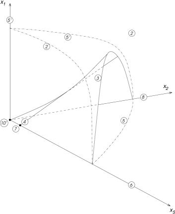
Fig. 1: Bifurcation diagram.

1. If $x_{2},x_{5}=0$, $x_{1}\neq 0$, then $\varphi(x_{1},x_{2},x_{5})\in E5^{\prime}$.

2. If $x_{1},x_{5}=0$, $x_{2}\neq 0$, then $\varphi(x_{1},x_{2},x_{5})\in E8$.

3. If $x_{1},x_{2}=0$, $x_{5}^{2}=-b_{1}^{2}/a_{4}$, then $\varphi(x_{1},x_{2},x_{5})\in E7$.

4. If $x_{1},x_{2}=0$, $x_{5}\neq 0$, $x_{5}^{2}\neq-b_{1}^{2}/a_{4}$, then $\varphi(x_{1},x_{2},x_{5})\in E6$.

5. If $x_{5}=0$, $x_{1},x_{2}\neq 0$, then $\varphi(x_{1},x_{2},x_{5})\in E5^{\prime}$.

6. If $x_{2}=0$, $x_{1},x_{5}\neq 0$, then $\varphi(x_{1},x_{2},x_{5})\in E2$.

7. If $x_{1}=0$, $x_{2},x_{5}\neq 0$, then $\varphi(x_{1},x_{2},x_{5})\in E5$.

8. If $x_{1},x_{2},x_{5}\neq 0$, $x_{1}=x_{2}x_{5}$, $x_{5}^{2}=-b_{1}^{2}/a_{4}$, then $\varphi(x_{1},x_{2},x_{5})\in E4$.

9. If $x_{1},x_{2},x_{5}\neq 0$, $x_{1}=x_{2}x_{5}$, $x_{5}^{2}\neq-b_{1}^{2}/a_{4}$, then $\varphi(x_{1},x_{2},x_{5})\in E3$.

10. If $x_{1},x_{2},x_{5}\neq 0$, $x_{1}\neq x_{2}x_{5}$, then $\varphi(x_{1},x_{2},x_{5})\in E2$.

4 Controllability

As it is well-known, controllability is a qualitative property playing a central role in many problems. In [2], one obtains an implicit characterization of the controllability of bimodal linear systems. Here, we will characterize explicitly the controllable unobservable bimodal linear systems for $n=2$ in a quite simple way (Corollary 10). The canonical forms for bimodal linear systems in Section 2 enable simple expressions for these conditions since they are invariant under admissible basis change transformations.

Theorem 6

([2]) Let us consider a bimodal linear system defined by $(A_{1},A_{2},B)$. Let us denote by $e\in M_{n\times 1}(\mathbb{R})$ the matrix such that $eC=A_{2}-A_{1}$. Then this system is controllable if, and only if,

1. $(A_{1},[B|e])$ is controllable.

2. $\left(v^{t}\ \mu_{i}\right)\left(\begin{array}[]{cc}\lambda I_{n}-A_{i}&B\\ C&0\end{array}\right)=0,\ \lambda\in\mathbb{R},v\not=0$ for $i=1,2\ \Rightarrow\ \mu_{1}\mu_{2}>0$ holds.

Next proposition proves that these conditions are invariant under admissible basis changes, so that they can be checked in the canonical form of the given system.

Proposition 7

Let us consider a controllable bimodal linear system defined by $(A_{1},A_{2},B)$. Then for all $S\in{\cal S}$, the system $(S^{-1}A_{1}S,S^{-1}A_{2}S,S^{-1}B)$ is controllable.

Proof. First, recall (see Proposition 1 (ii)) that the basis change $S$ preserves $C$ (that is, $CS=C$).

By a standard argument, from condition (1) it follows that the system $(S^{-1}AS,[S^{-1}B|S^{-1}e])$ is controllable. Then, it is sufficient to check

$$(S^{-1}e)C=(S^{-1}e)(CS)=S^{-1}(A_{2}-A_{1})S=S^{-1}A_{2}S-S^{-1}A_{1}S.$$

Concerning (2), let us see that the values $\mu_{i}$ are preserved when $S$ acts. Taking into account that

$$\left(\begin{array}[]{cc}\lambda I_{n}-S^{-1}A_{i}S&S^{-1}B\\ CS&0\end{array}\right)=\left(\begin{array}[]{cc}S^{-1}&\\ &I_{n}\end{array}\right)\left(\begin{array}[]{cc}\lambda I_{n}-A_{i}&B\\ C&0\end{array}\right)\left(\begin{array}[]{cc}S&\\ &I_{n}\end{array}\right)$$

it is obvious that

$$(v^{t}\ \mu_{i})\left(\begin{array}[]{cc}\lambda I_{n}-S^{-1}A_{i}S&S^{-1}B\\ CS&0\end{array}\right)=0$$

is equivalent to

$$(v^{t}S^{-1}\ \mu_{i})\left(\begin{array}[]{cc}\lambda I_{n}-A_{i}&B\\ C&0\end{array}\right)=0$$

 

Let us assume that $n=2$ and consider the unobservable system defined by $(A_{1},A_{2},B)$, where

$$A_{1}=\left(\begin{array}[]{cc}a_{1}&0\\ a_{2}&a_{4}\end{array}\right),A_{2}=\left(\begin{array}[]{cc}\gamma_{1}&0\\ \gamma_{2}&a_{4}\end{array}\right),B=\left(\begin{array}[]{c}b_{1}\\ b_{2}\end{array}\right)$$

The following theorem gives an equivalent condition to (2) in Theorem 6:

Proposition 8

Let us consider an unobservable bimodal linear system defined by $(A_{1},A_{2},B)$. With the above notation, if $n=2$, condition (2) in Theorem 6 is equivalent to

$$b_{1}\neq 0,\quad\Delta_{1}\Delta_{2}>0.$$

Proof. Condition (2) in Theorem 6 may be re-written as follows:

$$\left.\begin{array}[]{rl}b_{1}v_{1}+b_{2}v_{2}&=0\\ v_{2}(\lambda-a_{4})&=0\\ v_{1}(\lambda-a_{1})-v_{2}a_{2}+\mu_{1}&=0\end{array}\right\}$$

$$\left.\begin{array}[]{rl}b_{1}v_{1}+b_{2}v_{2}&=0\\ v_{2}(\lambda-a_{4})&=0\\ v_{1}(\lambda-\gamma_{1})-v_{2}\gamma_{2}+\mu_{2}&=0\end{array}\right\}$$

$\lambda\in\mathbb{R}$, $(v_{1},v_{2})\neq(0,0)$ implies $\mu_{1}\mu_{2}>0$.

1. If $b_{1}\neq 0$, then

   $$v_{1}=-b_{2},\quad v_{2}=b_{1},\quad\lambda=a_{4}.$$

   Hence,

   $$\mu_{1}=\Delta_{1},\quad\mu_{2}=\Delta_{2}$$

2. If $b_{1}=0$, the first and the second equations are verified by

   $$v_{1}\neq 0,\quad v_{2}=0,\quad\text{ any }\lambda\in\mathbb{R}$$

   so that any $\mu_{i}$ is possible, and (2) does not hold.

 

Corollary 9

In the conditions of Theorem 6, if $n=2$, condition (2) implies condition (1).

Proof. Condition (1) in Theorem 6 may be re-written as follows:

$$\mbox{\rm rk}\,\left(\begin{array}[]{cccc}b_{1}&a_{1}b_{1}&\gamma_{1}-a_{1}&a_{1}(\gamma_{1}-a_{1})\\ b_{2}&a_{2}b_{1}+a_{4}b_{2}&\gamma_{2}-a_{2}&a_{2}(\gamma_{1}-a_{1})+a_{4}(\gamma_{2}-a_{2})\end{array}\right)=2,$$

which clearly follows from $b_{1}\Delta_{1}\neq 0$.  

Our first main result follows from Theorem 6, Proposition 8 and Corollary 9.

Corollary 10

Let us consider an unobservable bimodal linear system defined by $(A_{1},A_{2},B)$. If $n=2$, this system is controllable if, and only if,

$$b_{1}\neq 0,\quad\Delta_{1}\Delta_{2}>0.$$

Remark From this formulation and Lemma 2 (1), it is obvious that if $(A_{1},A_{2},B)$ is controllable, then both subsystems $(A_{1},B)$ and $(A_{2},B)$ are controllable as well.

Next Table summarizes the results when the above condition is applied to the canonical form of each stratum:

Canonical form Controllability CF2 $b_{1}\neq 0$ and $\Delta_{1}\Delta_{2}>0$ CF3 $b_{1}\neq 0$ and $(a_{4}-a_{1})(a_{4}-\gamma_{1})>0$ CF4 Always uncontrollable CF5 $b_{1}\Delta_{2}>0$ CF5’ $b_{1}\Delta_{1}>0$ CF6 Always uncontrollable CF6’ Always uncontrollable CF7 Always uncontrollable CF7’ Always uncontrollable CF8 $a_{2}\gamma_{2}>0$ CF9 Always uncontrollable CF10 Always uncontrollable CF10’ Always uncontrollable CF11 Always uncontrollable CF11’ Always uncontrollable CF12 Always uncontrollable CF13 Always uncontrollable CF14 Always uncontrollable

Let us show an example to illustrate the study of the controllability of a bimodal linear system.

Example 2

Consider a bimodal linear system of type CF10’ whose canonical form is

$$A_{1}=\left(\begin{array}[]{rr}a_{4}&0\\ 0&a_{4}\end{array}\right),\;A_{2}=\left(\begin{array}[]{rr}a_{4}&0\\ 1&a_{4}\end{array}\right),\;B=\left(\begin{array}[]{c}b_{1}\\ 0\end{array}\right).$$

We consider the unobservable perturbation obtained in Example 1:

$$\varphi(x_{1},x_{2},x_{5})=\left(\left(\begin{array}[]{cc}a_{4}+x_{1}&0\\ x_{2}&a_{4}\end{array}\right),\left(\begin{array}[]{cc}a_{4}+x_{5}&0\\ 1&a_{4}\end{array}\right),\left(\begin{array}[]{c}b_{1}\\ -\frac{a_{4}}{b_{1}}x_{5}\end{array}\right)\right)$$

The controllable bimodal linear systems are those satisfying the condition in Corollary 10 which, taking into account that $b_{1}\neq 0$, is equivalent to

$$\left(x_{2}+\frac{a_{4}}{b_{1}^{2}}x_{1}x_{5}\right)\left(1+\frac{a_{4}}{b_{1}^{2}}x_{5}^{2}\right)>0,$$

which can be decomposed into:

• If $a_{4}>0$:  $x_{2}>-\frac{a_{4}}{b_{1}^{2}}x_{1}x_{5}$

• If $a_{4}<0$:  $x_{2}>-\frac{a_{4}}{b_{1}^{2}}x_{1}x_{5}$ and $x_{5}^{2}>-\frac{b_{1}^{2}}{a_{4}}$, or  $x_{2}<-\frac{a_{4}}{b_{1}^{2}}x_{1}x_{5}$ and $x_{5}^{2}<-\frac{b_{1}^{2}}{a_{4}}$

If $a_{4}<0$, the above condition is illustrated in Figure 2. Figure 3 summarizes examples 1 and 2.

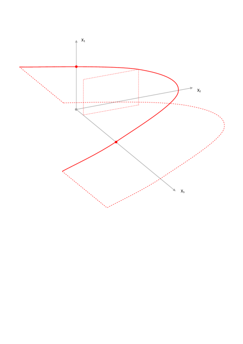
Fig. 2: Controllability.

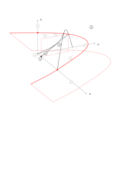
Fig. 3: Bifurcation diagram and Controllability. 

Finally, we will use the characterization of controllability in Corollary 10 and the canonical forms in Section 2 to prove that then the system is stabilizable, by means of a common feedback for both subsystems.

Theorem 11

Let us consider an unobservable planar bimodal linear system defined by $(A_{1},A_{2},B)$. If it is controllable, there is a feedback $F\in M_{1\times 2}(\mathbb{R})$ such that both subsystems $A_{1}+BF$ and $A_{2}+BF$ are stable.

Proof. We will detail the proof for the canonical form CF2. It works analogously for CF3, CF5, CF5’ and CF8.

By Corollary 10, the system

$$A_{1}=\left(\begin{array}[]{rr}a_{1}&0\\ 0&a_{4}\end{array}\right),\;A_{2}=\left(\begin{array}[]{rr}\gamma_{1}&0\\ 1&a_{4}\end{array}\right),\;B=\left(\begin{array}[]{c}b_{1}\\ b_{2}\end{array}\right)$$

is controllable if and only if

1. $b_{1}\neq 0$

2. $\Delta_{1}\Delta_{2}>0$

where $\Delta_{1}=(a_{4}-a_{1})b_{2},\quad\Delta_{2}=b_{1}+(a_{4}-\gamma_{1})b_{2}$.

We search $F=\left(\begin{array}[]{cc}f_{1}&f_{2}\end{array}\right)$ such that the matrices $A_{1}+BF$ and $A_{2}+BF$ have negative trace and positive determinant, that is to say:

$$b_{1}f_{1}+b_{2}f_{2}<-a_{1}-a_{4}$$

$$b_{1}f_{1}+b_{2}f_{2}<-\gamma_{1}-a_{4}$$

$$a_{4}b_{1}f_{1}+a_{1}b_{2}f_{2}>-a_{1}a_{4}$$

$$a_{4}b_{1}f_{1}+\gamma_{1}b_{2}f_{2}-b_{1}f_{2}>-\gamma_{1}a_{4}$$

We can change the variables $(f_{1},f_{2})$ by $(x,y)$ defined by

$$x = b_{1}f_{1}+b_{2}f_{2}$$

$$y = -(a_{4}b_{1}f_{1}+a_{1}b_{2}f_{2})$$

because (recall (i) and (ii))

$$\det\left(\begin{array}[]{cc}b_{1}&b_{2}\\ -a_{4}b_{1}&-a_{1}b_{2}\end{array}\right)=b_{1}\Delta_{1}\neq 0$$

Then:

$$f_{1}=-\frac{a_{1}x+y}{(a_{4}-a_{1})b_{1}},\quad f_{2}=\frac{a_{4}x+y}{(a_{4}-a_{1})b_{2}}$$

With this change of variables, the desired inequalities become:

$$x<-a_{1}-a_{4}$$

$$x<-\gamma_{1}-a_{4}$$

$$y<a_{1}a_{4}$$

$$a_{4}b_{1}\frac{a_{1}x+y}{(a_{4}-a_{1})b_{1}}+(b_{1}-\gamma_{1}b_{2})\frac{a_{4}x+y}{(a_{4}-a_{1})b_{2}}<\gamma_{1}\gamma_{4}$$

In order to see that there exist solutions $(x,y)$, it is sufficient that the coefficient of the variable $y$ in the last inequality be positive:

$$\frac{a_{4}b_{1}}{(a_{4}-b_{1})b_{1}}+\frac{b_{1}-\gamma_{1}b_{2}}{(a_{4}-a_{1})b_{2}}=\frac{1}{b_{1}\Delta_{1}}(a_{4}b_{1}b_{2}+b_{1}^{2}-\gamma_{1}b_{1}b_{2})=\frac{\Delta_{2}}{\Delta_{1}}>0$$

again by (ii).  

Acknowledgements

Preprint of an article submitted for consideration in IJBC ©2011 copyright World Scientific Publishing Company http://www.worldscinet.com/ijbc/