Weighted-Sum-Rate-Maximizing Linear Transceiver Filters for the K-User MIMO Interference Channel

Abstract

This letter is concerned with transmit and receive filter optimization for the K-user MIMO interference channel. Specifically, linear transmit and receive filter sets are designed which maximize the weighted sum rate while allowing each transmitter to utilize only the local channel state information. Our approach is based on extending the existing method of minimizing the weighted mean squared error (MSE) for the MIMO broadcast channel to the K-user interference channel at hand. For the case of the individual transmitter power constraint, however, a straightforward generalization of the existing method does not reveal a viable solution. It is in fact shown that there exists no closed-form solution for the transmit filter but simple one-dimensional parameter search yields the desired solution. Compared to the direct filter optimization using gradient-based search, our solution requires considerably less computational complexity and a smaller amount of feedback resources while achieving essentially the same level of weighted sum rate. A modified filter design is also presented which provides desired robustness in the presence of channel uncertainty.

I Introduction

To achieve high spectral efficiency, much effort has been focused on improving the achievable rate of multiple-input multiple-output (MIMO) interference channels [1, 2, 3]. A notable scheme in this area, the interference alignment (IA) technique of [4] confines all undesired interferences from other communication links into a pre-define subspace and achieves a maximum-capacity scaling. However, it is also known that IA can only offer a suboptimal sum rate at finite signal-to-noise ratios (SNRs) [3].

In this letter, we aim at maximizing the sum rate in the K-user MIMO interference channel. We consider two linear transceiver design methods. One is for the sum-power-usage-limit constraint and the other applies to the per-transmit-node power-usage constraint. The former can be viewed as a network-level constraint whereas the latter is more of a device-level constraint. In both designs, to maximize the weighted sum rate (WSR), we pursue minimization of the weighted mean squared error (WMSE). The idea of maximizing the WSR via receiver-side WMSE minimization was originally developed for the multi-user MIMO broadcast channel [5]. Our sum-power-constrained method could be seen as a generalization of the approach of [5] to cover the K-user MIMO interference channel and can be obtained as a direct extension of the method in [5]. However, our individual-power-constrained method is not a direct generalization of the method of [5] due to multiple power constraints. In fact, unlike in the case of the broadcast channel, we show that there is no closed-form solution for the minimum WMSE transmit filter, although a simple one-dimensional search for the power-adjusting parameter leads to the desired solution. Using simulation results and analysis, we verify that both proposed schemes achieve the maximum WSR with lower computational complexity than the gradient-based optimization of the transmit and receive filters [2]. Also, unlike in [2, 4, 6], our schemes require only the local channel state information (CSI) (i.e., each transmitter needs to know only the CSI of the links originating from itself whereas the MIMO interference channel precoder designs in [2, 4, 6] require the CSI for all links). Additionally, we discuss modified transceiver design that provides significant robustness in the presence of inaccurate CSI.

Related ideas for the MIMO interference channel can also be found in [3, 7, 8, 6, 9, 10]. In [3, 8], the minimum MSE (MMSE) transceiver is designed without considering different weights for the MSEs at multiple receivers. In [6] suboptimal MSE weights are used. In contrast, our weighted MMSE transceiver design relies on a set of MSE weights that provides a direct link between the weighted MMSE (WMMSE) and WSR criteria. The WMMSE-based weighted utility maximization is also considered in [7], but there only a single data stream is assumed between a given user pair. A very similar idea on maximizing WSR via WMSE minimization under the individual power constraint has been discussed in [9]. But, unlike in our approach, the inter-dependency between the transmit-power-adjusting Lagrange multiplier and the precoding matrix has not been considered in [9]. In our individual-power-constrained transceiver design, this inter-dependency is handled by introducing one-dimensional search for the Lagrange multiplier. This means that the method of [9] requires recursive optimization based on exchanges of filter-setting information among all transmitters. Our method does not require recursive filter adjustment and no data exchanges are needed among transmitters. Finally, we present a modified transceiver design method for the imperfect-CSI environment and analyze the computational complexity as well as the required feedback amount in comparison with the gradient descent method [2].

The following notations are used. We employ upper case boldface letters for matrices and lower case boldface for vectors. For any general matrix, ${\bf{X}}$, ${\bf{X}}^{T}$, ${\bf{X}}^{*}$, ${\bf{X}}^{H}$, $\text{Tr}({\bf{X}})$, $\text{det}({\bf{X}})$, $\text{vec}($X$)$, $\text{SVD}($X$)$ denote the transpose, the conjugate, the Hermitian transpose, the trace, the determinant, the stack columns, and the singular value decomposition of ${\bf{X}}$, respectively. The symbol ${||}\cdot{||}_{2}$ indicates the 2-norm of a vector. The symbol ${\bf{I}}_{n}$ denotes an identity matrix of size $n$.

II System Model

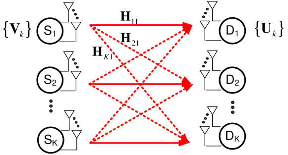
Figure 1: K-user MIMO interference channel

We consider the MIMO interference channel where precoding can only be done over one transmission slot. As shown in Fig. 1, $K$ source nodes simultaneously transmit independent data streams to their desired destination nodes and generate co-channel interference to all other undesired nodes. In this system each source node $\{\textsf{S}_{k}\}$ is equipped with $M$ antennas and each destination node $\{\textsf{D}_{k}\}$ has $N$ antennas $(k\in\{1\sim K\})$. The MIMO channels from $\textsf{S}_{i}$ to $\textsf{D}_{j}$ are modelled by ${\bf{H}}_{ji}\in{\mathcal{C}}^{N\times M}$ $(i,j\in\{1\sim K\})$ whose coefficients are independent and identically distributed (i.i.d) complex Gaussian random variables with $\mathcal{CN}(0,\sigma_{h}^{2})$. We assume that the channel information is only locally available, i.e., each node knows only the coefficients for the channel link originating from itself. Note that the precoder designs of [2, 4, 6] are based on the availability of the global channel information. Let ${\bf{s}}_{k}\in{\mathcal{C}}^{d\times 1}$ denote the symbol vector from $\textsf{S}_{k}$ with $\mathbb{E}[{\bf{s}}_{k}{\bf{s}}_{k}^{H}]={\bf{I}}_{d}$ where $d$ is the number of data streams for $\textsf{D}_{k}$, $d\leq M,N$ and the value of $d$ is chosen to meet the feasibility of degree of freedom [11]. Also ${\bf{V}}_{k}\in{\mathcal{C}^{M\times d}}$ denotes the precoding matrix for $\textsf{S}_{k}$. Then, the $N\times 1$ received signal vector at $\textsf{D}_{k}$ is represented as

$${\bf{y}}_{k}={\bf{H}}_{kk}{\bf{V}}_{k}{\bf{s}}_{k}+\sum_{i\neq k}^{K}{\bf{H}}_{ki}{\bf{V}}_{i}{\bf{s}}_{i}+{\bf{n}}_{k},$$ (1)

where ${\bf{n}}_{k}$ denotes the i.i.d complex Gaussian noise vector at $\textsf{D}_{k}$ with $\mathcal{CN}({\bf{0}},\sigma_{n}^{2}{\bf{I}}_{N})$. Then, $\textsf{D}_{k}$ combines its received signal with ${\bf{U}}_{k}\in{\mathcal{C}^{d\times N}}$ to decode the desired signals:

$$\hat{\bf{s}}_{k}={\bf{U}}_{k}{\bf{y}}_{k}={\bf{U}}_{k}{\bf{H}}_{kk}{\bf{V}}_{k}{\bf{s}}_{k}+{\bf{U}}_{k}\sum_{i\neq k}^{K}{\bf{H}}_{ki}{\bf{V}}_{i}{\bf{s}}_{i}+{\bf{U}}_{k}{\bf{n}}_{k}.$$ (2)

Our goal is to find $\{{\bf{V}}_{k}\}$ and $\{{\bf{U}}_{k}\}$ that maximize the WSR under the sum-power constraint and also the individual-power constraint. We assume a unit noise variance ($\sigma_{n}^{2}=1$) without losing generality.

III Weighted Sum Rate Maximization

First consider finding $\{{\bf{V}}_{k}\}$ that maximizes

$$\sum_{k=1}^{K}\mu_{k}R_{k}\quad\text{subject to }\sum_{k}\text{Tr}({\bf{V}}_{k}{\bf{V}}_{k}^{H})=P_{T}\quad\text{or}\quad\text{Tr}({\bf{V}}_{k}{\bf{V}}_{k}^{H})=P_{k}\quad\forall k$$ (3)

where the subscript $k$ points the source node and its intended destination node, $\mu_{k}$ denotes the weight, $R_{k}$ is the achievable rate, $P_{T}$ represents the maximum sum power allowed for all transmitters and $P_{k}$ is the $k$-th node’s maximum transmit power. With Gaussian signaling, the achievable rate takes the well-known form:

$$\quad R_{k}=\text{log }\Big{\{}\text{det}\Big{(}{\bf{I}}_{N}+{\bf{\Phi}}_{k}^{-1}{\bf{H}}_{kk}{\bf{V}}_{k}{\bf{V}}_{k}^{H}{\bf{H}}_{kk}^{H}\Big{)}\Big{\}},$$ (4)

where ${\bf{\Phi}}_{k}={\bf{I}}_{N}+\sum_{i\neq k}^{K}{\bf{H}}_{ki}{\bf{V}}_{i}{\bf{V}}_{i}^{H}{\bf{H}}_{ki}^{H}$. We attempt to solve this WSR maximization problem by minimizing the weighted receiver MSE, as has been done for the MIMO broadcast channel [5]. This approach was also attempted for the K-user MIMO interference channel in [9] under the individual-power constraint, but our solution is different as elaborated below.

III-A Relationship between achievable rate and error covariance matrix

To understand the link between the WSR maximization problem and the WMSE minimization problem in the K-user MIMO interference channel, we need to clarify the relationship between the achievable rate and the error covariance matrix. This argument is parallel to one given in [5] for the MIMO broadcast channel. For the MMSE receive filter at $\textsf{D}_{k}$, we write

$${\bf{U}}_{k}^{(MMSE)}= \arg\min\mathbb{E}||{\bf{U}}_{k}{\bf{y}}_{k}-{\bf{s}}_{k}||_{2}^{2}$$

$$= {\bf{V}}_{k}^{H}{\bf{H}}_{kk}^{H}(\sum_{i=1}^{K}{\bf{H}}_{ki}{\bf{V}}_{i}{\bf{V}}_{i}^{H}{\bf{H}}_{ki}^{H}+{\bf{I}}_{N})^{-1},$$ (5)

and the error matrix for $\textsf{D}_{k}$ is given by

$${\bf{E}}_{k}= \mathbb{E}\{({\bf{U}}_{k}^{(MMSE)}{\bf{y}}_{k}-{\bf{s}}_{k})({\bf{U}}_{k}^{(MMSE)}{\bf{y}}_{k}-{\bf{s}}_{k})^{H}\}$$

$$= ({\bf{I}}_{N}+{\bf{\Phi}}_{k}^{-1}{\bf{H}}_{kk}{\bf{V}}_{k}{\bf{V}}_{k}^{H}{\bf{H}}_{kk}^{H})^{-1}.$$ (6)

Comparing (4) and (6), the relationship between the achievable rate and the error covariance matrix is established as:

$$R_{k}=\text{log }\{\text{det}({\bf{E}}_{k}^{-1})\}$$ (7)

which, not surprisingly, is identical to the relationship between the rate and the error covariance matrix for the case of the MIMO broadcast channel [5]. Apparently, though, the error covariance matrix ${\bf{E}}_{k}$ here is different from that of the broadcast channel due to the presence of multiple sources. Note that this relationship between the achievable rate and the error covariance matrix holds for any $\{{\bf{V}}_{k}\}$, implying that (7) is true with either transmit power constraint.

III-B MSE weight design

Now consider finding $\{{\bf{V}}_{k}\}$ that solves the following WMMSE problem:

$$\min\sum_{k=1}^{K}\text{Tr}({\bf{W}}_{k}{\bf{E}}_{k})\quad\text{subject to }\sum_{k}\text{Tr}({\bf{V}}_{k}{\bf{V}}_{k}^{H})=P_{T}\quad\text{or}\quad\text{Tr}({\bf{V}}_{k}{\bf{V}}_{k}^{H})=P_{k}\quad\forall k,$$ (8)

where ${\bf{W}}_{k}\in\mathcal{C}^{d\times d}$ represents the MSE weight. Again following the argument of [5], the MSE weights can be chosen so that both WSR and WMMSE problems have a common solution. For this, set up the Lagrangians for (3) and (8):

$$\mathcal{L}_{WSR}=-\sum_{k=1}^{K}\mu_{k}R_{k}+\theta\lambda(\sum_{k=1}^{K}\text{Tr}({\bf{V}}_{k}{\bf{V}}_{k}^{H})-P_{T})+(1-\theta)\Big{(}\sum_{k=1}^{K}{\lambda}_{k}(\text{Tr}({\bf{V}}_{k}{\bf{V}}_{k}^{H})-P_{k})\Big{)}$$

and

$$\mathcal{L}_{WMSE}=\sum_{k=1}^{K}\text{Tr}({\bf{W}}_{k}{\bf{E}}_{k})+\theta\lambda(\sum_{k=1}^{K}\text{Tr}({\bf{V}}_{k}{\bf{V}}_{k}^{H})-P_{T})+(1-\theta)\Big{(}\sum_{k=1}^{K}{\lambda}_{k}(\text{Tr}({\bf{V}}_{k}{\bf{V}}_{k}^{H})-P_{k})\Big{)}$$

respectively, where $\theta$ selects the desired power constraint (’$\theta=1$’ for the sum power constraint and ’$\theta=0$’ for the individual power constraint), $\lambda$ and $\{\lambda_{k}\}$ denote the Lagrange multipliers for the two transmit power constraints. Next, equate their gradients obtained via the matrix derivative formulas: $d\{\text{ln}(\text{det}({\bf{X}}))\}=\text{Tr}\{{\bf{X}}^{-1}d({\bf{X}})\}$, $d\{\text{Tr}({\bf{X}})\}=\text{Tr}\{d({\bf{X}})\}$, $\text{vec}\{d({\bf{X}})\}=d\{\text{vec}({\bf{X}})\}$, $\text{Tr}({\bf{X}}^{T}{\bf{Y}})=\text{vec}({\bf{X}})^{T}\text{vec}({\bf{Y}})$. Subsequently, the resulting MSE weight can be found as

$${\bf{W}}_{k}=\frac{\mu_{k}}{\text{ln(2)}}{\bf{E}}_{k}^{-1}.$$ (9)

Note that the choice of the MSE weights $\{{\bf{W}}_{k}\}$ is irrelevant to the transmit power constraint, which makes sense as $\{{\bf{W}}_{k}\}$ are receiver-side design parameters.

III-C Sum power constrained precoder design

We are now ready to find the transmit precoding matrix that minimizes the WMSE under the sum-power constraint, i.e., find $\{{\bf{V}}_{k}\}$ that minimizes

$$\sum_{k=1}^{K}\mathbb{E}[\text{Tr}\{{\bf{W}}_{k}({\bf{s}}_{k}-\beta^{-1}\hat{\bf{s}}_{k})({\bf{s}}_{k}-\beta^{-1}\hat{\bf{s}}_{k})^{H}\}]\quad\text{subject to }\sum_{k}\text{Tr}({\bf{V}}_{k}{\bf{V}}_{k}^{H})=P_{T}$$ (10)

where $\{{\bf{W}}_{k}\}$ is set according to (9) and $\beta$ is a scaling parameter. With matrix derivative formulas, the WMMSE transmit filter that satisfies (10) can be shown to be

$${\bf{V}}_{k}=\beta{\bf{V}}_{k}^{{}^{\prime}},$$ (11)

where ${\bf{V}}_{k}^{{}^{\prime}}=\Big{(}{\bf{\Psi}}_{k}+\frac{\sum_{i}\text{Tr}({\bf{W}}_{i}{\bf{U}}_{i}{\bf{U}}_{i}^{H})}{P_{T}}{\bf{I}}_{M}\Big{)}^{-1}{\bf{H}}_{kk}^{H}{\bf{U}}_{k}^{H}{\bf{W}}_{k}$, ${\bf{\Psi}}_{k}=\sum_{i=1}^{K}{\bf{H}}_{ik}^{H}{\bf{U}}_{i}^{H}{\bf{W}}_{i}{\bf{U}}_{i}{\bf{H}}_{ik}$, and $\beta=\sqrt{\frac{P_{T}}{\sum_{k}\text{Tr}({\bf{{V}}}_{k}^{{}^{\prime}}{{\bf{{V}}}_{k}^{{}^{\prime}}}^{H})}}$.

This result is a rather straightforward generalization of the WMMSE precoder in the broadcast channel. It can indeed be seen that setting ${\bf{H}}_{ki}={\bf{H}}_{kk}$ for all $i$, our solutions (5), (9), and (11) reduce to the respective receive filter, MSE weight and transmit filter solutions obtained for the multi-user MIMO broadcast channels through WMSE minimization [5].

III-D Individual power constrained transceiver design

Now let us consider the individual-power-constrained network. We proceed to find the transmit filter that minimizes the weighted MSE:

$$\sum_{k=1}^{K}\mathbb{E}[\text{Tr}\{{\bf{W}}_{k}({\bf{s}}_{k}-\hat{\bf{s}}_{k})({\bf{s}}_{k}-\hat{\bf{s}}_{k})^{H}\}]\quad\text{subject to }\text{Tr}({\bf{V}}_{k}{\bf{V}}_{k}^{H})=P_{k}\quad\forall k.$$ (12)

Again equating the gradients of the Lagrangians corresponding to the WMMSE and WSR maximization procedures and using the matrix derivative formulas, the WMMSE transmit filter at $\textsf{S}_{k}$ is found as:

$${\bf{{V}}}_{k}= \Big{(}{\bf{\Psi}}_{k}+\lambda_{k}{\bf{I}}_{M}\Big{)}^{-1}{\bf{H}}_{kk}^{H}{\bf{U}}_{k}^{H}{\bf{W}}_{k}$$ (13)

where $\lambda_{k}$ is set to satisfy the transmit power constraint at $\textsf{S}_{k}$ and again $\{{\bf{W}}_{k}\}$ are as given in (9). Unlike the sum-power-constrained WMMSE precoders of (11), for which the power control parameters are found in closed form, here we resort to a numerical method to find $\lambda_{k}$, due to the inter-dependency between ${\bf{{V}}}_{k}$ and $\lambda_{k}$ in (13). Fortunately, based on the following lemma, $\lambda_{k}$ can be found with simple one-dimensional (1-D) numerical search.

Lemma 1

The per-node transmit power, $\text{Tr}({\bf{V}}_{k}(\lambda_{k}){\bf{V}}_{k}(\lambda_{k})^{H})$, is a monotonically decreasing function of $\lambda_{k}$.

Proof:

Let $\text{SVD}({\bf{\Psi}}_{k})={\bf{Q}}_{k}{\bf{\Sigma}}_{k}{\bf{Q}}_{k}^{H}$. Then, the transmit power at $\textsf{S}_{k}$ is given by

$$\text{Tr}\{({\bf{V}}_{k}(\lambda_{k}){\bf{V}}_{k}(\lambda_{k})^{H}\}= \text{Tr}\{({\bf{Q}}_{k}{\bf{\Sigma}}_{k}{\bf{Q}}_{k}^{H}+\lambda_{k}{\bf{I}_{M}})^{-1}{\bf{H}}_{kk}^{H}{\bf{U}}_{k}^{H}{\bf{W}}_{k}{\bf{U}}_{k}{\bf{H}}_{kk}({\bf{Q}}_{k}{\bf{\Sigma}}_{k}{\bf{Q}}_{k}^{H}+\lambda_{k}{\bf{I}_{M}})^{-1}\}$$

$$= \text{Tr}\{({\bf{\Sigma}}_{k}+\lambda_{k}{\bf{I}_{M}})^{-2}{\bf{Q}}_{k}^{H}{\bf{H}}_{kk}^{H}{\bf{U}}_{k}^{H}{\bf{W}}_{k}{\bf{U}}_{k}{\bf{H}}_{kk}{\bf{Q}}_{k}\}$$

$$= \sum_{i=1}^{K}\frac{[{\bf{\Pi}}_{k}]_{i,i}}{(\sigma_{k,i}+\lambda_{k})^{2}},$$ (14)

where ${\bf{\Pi}}_{k}={\bf{Q}}_{k}^{H}{\bf{H}}_{kk}^{H}{\bf{U}}_{k}^{H}{\bf{W}}_{k}{\bf{U}}_{k}{\bf{H}}_{kk}{\bf{Q}}_{k}$ , $[{\bf{\Pi}}_{k}]_{i,i}$ is the $ii$-th element of ${\bf{\Pi}}_{k}$, and $\sigma_{k,i}$ is the $i$-th element of ${\bf{\Sigma}}_{k}$. Because $\lambda_{k}\geq 0$, $\text{Tr}\{{\bf{V}}_{k}(\lambda_{k}){\bf{V}}_{k}(\lambda_{k})^{H}\}$ is monotonically decreasing with $\lambda_{k}$. ∎

Note that the proper set of MSE weights for the K-user MIMO interference channel has already been derived in [9] in the process of establishing a connection between the WMMSE problem and the WSR maximization problem. In [9], though, the transmitter $\textsf{S}_{k}$ is expressed as a function of itself as well as transmitters at the other nodes, i.e. ${\bf{V}}_{k}=f(\{{\bf{V}}_{1},\cdots,{\bf{V}}_{K}\})$. The consequence of this formulation is that the transmitter solution in [9] cannot be found without recursive calculation and additional filter-setting information exchanges among all transmit nodes. In contrast, our transmit filter design is based on a clear recognition of the inter-dependency between $\lambda_{k}$ and ${\bf{V}}_{k}$, and as a result the proposed transmit filter (13) can be found through a simple 1-D numerical search with no additional information ($\{{\bf{V}}_{l}\}$ ($l\neq k$)) exchanges needed among the transmit nodes.

III-E Iterative algorithm to maximize the weighted sum rate

In the previous sections, we found the MSE weights and then subsequently WMMSE receive and transmit filters with both the sum-power constraint and the individual-power constraint. Each of three sets of parameters - MSE weights, transmit filters and receive filters - is derived assuming the other sets are given. In practice, to find optimum WSR solutions, the inter-dependencies between the parameters are handled with the following iterative or alternating optimization algorithm.

Algorithm 1 Obtaining the optimal WSR transceivers via the WMMSE criterion

  Initialize $l=0$ and $\{{\bf{V}}_{k}^{(0)}\}$, calculate ${R}_{sum}^{(0)}$.

  repeat

     $l:=l+1$

     Step 1: Calculate ${\bf{U}}_{k}^{(l)}|\{{\bf{V}}_{i}^{(l-1)}\}$ for all $k$ using (5).

     Step 2: Calculate ${\bf{W}}_{k}^{(l)}|\{{\bf{V}}_{i}^{(l-1)}\}$ for all $k$ using (9).

     Step 3: Calculate ${\bf{V}}_{k}^{(l)}|\{{\bf{U}}_{i}^{(l)}\}$, $\{{\bf{W}}_{i}^{(l)}\}$ for all $k$ using (11) for the sum power constrained case or (13) for the individual power constrained case.

  until $|{R}_{sum}^{(l)}-{R}_{sum}^{(l-1)}|<\epsilon$, where $\epsilon$ is some arbitrarily small value and $R_{sum}=\sum_{k}\mu_{k}R_{k}$.

The algorithm is common to both the sum-power-constrained design and the individual-power-constrained design. This algorithm is provably convergent to a local optimum; this can be shown by proving monotonic convergence of an equivalent optimization problem based on expanding the WSR maximization problem of (3) to add the MMSE weights and receive filters as optimization variables, as has been done for the MIMO broadcast channel in [5]. We note, however, that this algorithm does not guarantee the global optimal solution, since the WMMSE minimization (8) is not jointly convex over all input variables. To reasonably approach the optimal solution one must resort to repeated runs of the algorithm using different initial settings, or, for computationally efficient initialization, choose $\{{\bf{V}}_{k}^{(0)}\}$ in Step 1 from the right singular matrices of $\{{\bf{H}}_{kk}\}$ or from random matrices generated according to the normal distribution with zero mean and unit variance [8].

IV Robust transceiver design for imperfect channel information

In practical scenarios, mismatch between the true channel $\{{\bf{H}}_{ij}\}$ and the estimated channel (denoted by $\{\tilde{\bf{H}}_{ij}\}$) is inevitable because of the channel estimation errors [12]. In this section, we design robust transceivers for mitigating the performance degradation caused by channel mismatch. We assume that $\{\tilde{\bf{H}}_{ij}\}$ is related to $\{{\bf{H}}_{ij}\}$ by $\tilde{\bf{H}}_{ij}={\bf{H}}_{ij}+{\bf{\Delta}}_{ij}$ where the elements of ${\bf{\Delta}}_{ij}$ are independent and identically distributed (i.i.d.) complex Gaussian random variables with variance $\sigma_{\Delta}^{2}$ [12]. Then, the received signal can be rewritten as

$${\tilde{{\bf{s}}}}_{k}={\tilde{\bf{U}}}_{k}({\tilde{\bf{H}}}_{kk}-{\bf{\Delta}}_{kk}){\tilde{\bf{V}}}_{k}{\bf{s}}_{k}+{\tilde{\bf{U}}}_{k}\sum_{i\neq k}^{K}({\tilde{\bf{H}}}_{ki}-{\bf{\Delta}}_{ki}){\tilde{\bf{V}}}_{i}{{\bf{s}}}_{i}+{\tilde{\bf{U}}}_{k}{\bf{n}}_{k}$$ (15)

where $\{{\tilde{\bf{V}}}_{k}\}$ and $\{{\tilde{\bf{U}}}_{k}\}$ are computed from $\{{\tilde{\bf{H}}}_{ij}\}$ with no knowledge of the presence of $\{{\bf{\Delta}}_{ij}\}$. We try to mitigate the effect of channel mismatch by minimizing the appropriate metrics averaged over ${\bf{\Delta}}_{ij}$’s.

IV-1 Modified MSE weight

Following the design procedure in previous sections, a modified version of the MMSE receiver filter is found as ${\tilde{\bf{U}}}_{k}={\tilde{\bf{V}}}_{k}^{H}{\tilde{\bf{H}}}_{kk}^{H}(\sum_{i=1}^{K}{\tilde{\bf{H}}}_{ki}{\tilde{\bf{V}}}_{i}{\tilde{\bf{V}}}_{i}^{H}{\tilde{\bf{H}}}_{ki}^{H}+\sum_{i=1}^{K}\sigma_{\Delta}^{2}\text{Tr}({\bf{\Lambda}}_{{\tilde{\bf{V}}}_{i}}){\bf{I}}_{N}+{\bf{I}}_{N})^{-1}$, where $\text{SVD}({\tilde{\bf{V}}}_{i}{\tilde{\bf{V}}}_{i}^{H})={\bf{Q}}_{i}{\bf{\Lambda}}_{{\tilde{\bf{V}}}_{i}}{\bf{Q}}_{i}^{H}$. The modified MSE weights that force the optimum solutions of the WSR maximization and WMMSE problems to be identical are derived as ${\tilde{\bf{W}}}_{k}=\frac{\mu_{k}}{\text{ln}(2)}{\tilde{\bf{E}}}_{k}^{-1}$, where ${\tilde{\bf{E}}}_{k}=({\bf{I}}_{N}+{\tilde{\bf{\Phi}}}_{k}^{-1}{\tilde{\bf{H}}}_{kk}{\tilde{\bf{V}}}_{k}{\tilde{\bf{V}}}_{k}^{H}{\tilde{\bf{H}}}_{kk}^{H})^{-1}$ and ${\tilde{\bf{\Phi}}_{k}}={\bf{I}}_{N}+\sum_{i\neq k}^{K}{\tilde{\bf{H}}}_{ki}{\tilde{\bf{V}}}_{i}{\tilde{\bf{V}}}_{i}^{H}{\tilde{\bf{H}}}_{ki}^{H}+\sum_{i=1}^{K}\sigma_{\Delta}^{2}\text{Tr}({\bf{\Lambda}}_{{\tilde{\bf{V}}}_{i}}){\bf{I}}_{N}$.

IV-2 Robust transceiver design with the sum power constraint

The modified transmit filters are derived based on the following optimization problem:

$$\min\sum_{k=1}^{K}\mathbb{E}[\text{Tr}\{{\tilde{\bf{W}}}_{k}({\bf{s}}_{k}-{\tilde{\beta}}^{-1}{\tilde{{\bf{s}}}}_{k})({\bf{s}}_{k}-{\tilde{\beta}}^{-1}{\tilde{{\bf{s}}}}_{k})^{H}\}]\quad\text{subject to }\sum_{k}\text{Tr}({\tilde{\bf{V}}}_{k}{\tilde{\bf{V}}}_{k}^{H})=P_{T}.$$ (16)

Utilizing matrix derivative formulas, the resultant modified-WMMSE transmit filters are obtained as

$${\tilde{\bf{V}}}_{k}={\tilde{\beta}}{\tilde{\bf{V}}}_{k}^{{}^{\prime}},$$ (17)

where ${\tilde{\bf{V}}}_{k}^{{}^{\prime}}=\Big{(}{\tilde{\bf{\Psi}}}_{k}+\frac{\sum_{i=1}^{K}\text{Tr}({\tilde{\bf{W}}}_{i}{\tilde{\bf{U}}}_{i}{\tilde{\bf{U}}}_{i}^{H})}{P_{T}}{\bf{I}}_{M}+\sum_{i=1}^{K}\sigma_{\Delta}^{2}\text{Tr}({\bf{\Lambda}}_{{\tilde{\bf{U}}}_{i}}){\bf{I}}_{M}\Big{)}^{-1}{\tilde{\bf{H}}}_{kk}^{H}{\tilde{\bf{U}}}_{k}^{H}{\tilde{\bf{W}}}_{k}$, ${\tilde{\beta}}=\sqrt{\frac{P_{T}}{\sum_{k}\text{Tr}({\tilde{\bf{V}}}_{k}^{{}^{\prime}}{{\tilde{\bf{V}}}_{k}^{{}^{\prime}H}})}}$, ${\tilde{\bf{\Psi}}}_{k}=\sum_{i=1}^{K}{\tilde{\bf{H}}}_{ik}^{H}{\tilde{\bf{U}}}_{i}^{H}{\tilde{\bf{W}}}_{i}{\tilde{\bf{U}}}_{i}{\tilde{\bf{H}}}_{ik}$, and $\text{SVD}({\tilde{\bf{U}}}_{i}^{H}{\tilde{\bf{W}}}_{i}{\tilde{\bf{U}}}_{i})={\bf{Q}}_{i}^{{}^{\prime}}{\bf{\Lambda}}_{{\tilde{\bf{U}}}_{i}}{\bf{Q}}_{i}^{{}^{\prime}H}$.

IV-3 Robust transceiver design with the individual power constraint

The optimization problem to derive the modified precoder is

$$\min\sum_{k=1}^{K}\mathbb{E}[\text{Tr}\{{\tilde{\bf{W}}}_{k}({\bf{s}}_{k}-{\tilde{{\bf{s}}}}_{k})({\bf{s}}_{k}-{\tilde{{\bf{s}}}}_{k})^{H}\}]\quad\text{subject to }\text{Tr}({\tilde{\bf{V}}}_{k}{\tilde{\bf{V}}}_{k}^{H})=P_{k}\quad\forall k.$$ (18)

With the matrix derivative formulas, the modified-WMMSE transmit precoder at $\textsf{S}_{k}$ with the individual power constraint is written as

$${\tilde{\bf{{V}}}}_{k}= \Big{(}{\tilde{\bf{\Psi}}}_{k}+{\tilde{\lambda}}_{k}{\bf{I}}_{M}+\sum_{i=1}^{K}\sigma_{\Delta}^{2}\text{Tr}({\bf{\Lambda}}_{{\tilde{\bf{U}}}_{i}}){\bf{I}}_{M}\Big{)}^{-1}{\tilde{\bf{H}}}_{kk}^{H}{\tilde{\bf{U}}}_{k}^{H}{\tilde{\bf{W}}}_{k}$$ (19)

where the power control parameter ${\tilde{\lambda}}_{k}$ is also found by numerical 1-D search.

Note that, for the above derivations, we have assumed that the value of the channel error variance $\sigma_{\Delta}^{2}$ is perfectly known. In the practical systems, the channel error variance can be estimated through an appropriate statistical approach [13]. Below, we also present numerical performance results corresponding to the cases where the error variance is not perfectly known.

V Discussion: Computational complexity, channel state information

In this section, we analyze computational complexity and required feedback resources. For comparison, we also analyze those of the gradient descent method of [2].

V-A Computational complexity

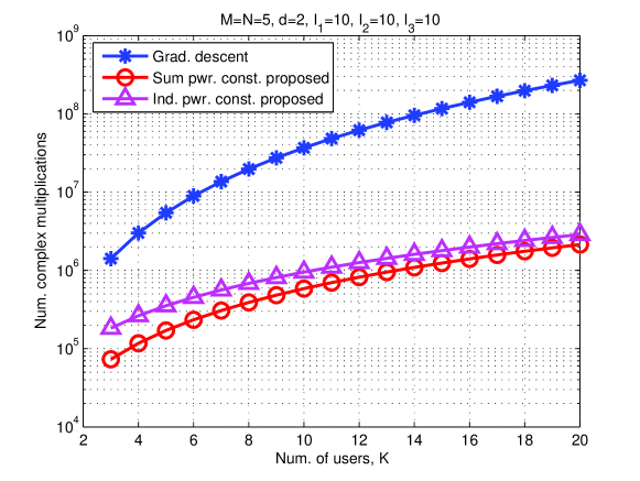
Figure 2: Complexity comparison between the gradient-descent-based method and the proposed methods

We consider the number of complex multiplications as a complexity measure. As summarized in the Table I, the number of complex multiplications is proportional to the number of iterations. The proposed method with the sum-power constraint which has a single iteration loop is computationally the most efficient. Whereas both the proposed method with the individual-power constraint and the gradient descent method require double iteration loops, i.e., the outer loop for updating the sum rate and the inner loop for adjusting the Lagrange multiplier (in the case of the proposed method) or for updating the step size (in the case of the gradient-based method). Calculating the gradient and adjusting the step size require more computational resources. According to simulation, when SNR = $10$ dB which is in the mid SNR regime, $K=4$, $M=N=5$, and $d=2$, the minimum average numbers of iteration for the convergence of sum rate, updating the step size of gradient method and 1-D search with bisection method are $10$, $10$ and $10$, respectively. In accordance with these, $I_{1}=10$, $I_{2}=10$ and $I_{3}=10$ are chosen. The symbols $c_{N}^{1}$, $c_{NM}^{2}$ and $c_{N}^{3}$ denote the computational complexity of a matrix inversion of $N\times N$ matrix, a singular value decomposition of $N\times M$ matrix, and a Cholesky factorization of $N\times N$ matrix, respectively. The corresponding values for those variables are $\frac{2}{3}N^{3}$, $7NM^{2}+4M^{3}$, and $\frac{1}{3}N^{3}$, respectively [14]. Fig. 2 shows comparison when $M=N=5$ and $d=2$ . As expected, for the same WSR values the proposed method with the sum-power constraint has the least complexity while the gradient descent algorithm is the most computationally complex.

V-B The amount of required feedback information

To find the optimized transmit precoders, each transmit node requires feedback information. As illustrated in Table II, feedback information is composed of CSI and coefficients for filter updating. For a given transmission slot, CSI feedback is required once, but the filter coefficients are updated several times due to the iterative optimization algorithm. Although the proposed method requires a larger amount of feedback information for the iteratively updated coefficients such as MSE weights $\{{\bf{W}}_{k}\}$ and receive filter coefficients $\{{\bf{U}}_{k}\}$ than the gradient descent method does, the amount of CSI feedback for the proposed method is smaller than for the gradient descent method. This is because, unlike the global CSI requirement of the gradient-based method, the proposed methods need only local CSI. From Table II, we observe that as the network size grows (i.e., $K$ increases) the required feedback resources for local CSI and coefficient updating increase linearly, but those for global CSI increases quadratically. Fig. 3 clearly shows that with $I_{1}=10$ the proposed methods are advantageous in terms of required feedback resources, especially for larger $K$. Note that, for the transmit power adjustment, the sum-power-constrained method additionally requires iterative update of the scalar parameter $\text{Tr}\{\sum_{i\neq k}{\bf{V}}_{i}^{{}^{\prime}}{\bf{V}}_{i}^{{}^{\prime}H}\}$, but the size of this parameter is negligible compared to other matrix parameters.

VI Numerical Results

In this section, we provide the numerical results related to the WSR performances. The SNR for the sum-power-constrained network, $\text{SNR}=\frac{P_{T}\sigma_{h}^{2}}{K\sigma_{n}^{2}}$, and that for the individual power constrained network, $\text{SNR}_{k}=\frac{P_{k}\sigma_{h}^{2}}{\sigma_{n}^{2}},\forall k$, are derived assuming $P_{T}=K$, $P_{k}=1\forall k$ and $\sigma_{n}^{2}=1$, i.e., $\text{SNR}=\text{SNR}_{k}=\sigma_{h}^{2}$. The results are averaged over 1000 independent trials. Fig. 4 shows the average WSR performance of the proposed methods for $M=N=5$ (when $K=4$), $M=N=6$ (when $K=5$), and $d=2$. For fairness, all schemes are initialized with the right singular matrices of the intended channels. For the sum-power constraint, we set the weights to be $\mu_{1}=2$ and $\mu_{k}=0.25$ $(k\neq 1)$, which were chosen rather arbitrarily except that $\mu_{1}$ is made considerably larger than $\mu_{k}$ to bring out the performance advantage of the sum-power constraint. The performance of the sum power constraint method should be better than that of the individual power constraint method because the former, which is less stringent, is able to allocate more power to the higher weighted transmitter to maximize the WSR. When the weights are equal, $\mu_{k}=1$ $\forall k$, the performance of both proposed schemes and that of the conventional gradient descent method are nearly identical. Note that, as explained in section IV, the proposed methods achieve these performances with less computational complexity and a smaller amount of feedback resources than the gradient descent method. Compared to the performance of the MMSE transceiver without the MSE weights [8, 3] (curves labelled ”Simple MMSE”), the advantage of designed MSE weights is clearly shown as SNR grows. Fig. 5 demonstrates the effectiveness of the robust design with either transmit power constraint in presence of channel uncertainty when $K=4$ and $\sigma_{\Delta}^{2}=0.1\sigma_{h}^{2}$. As SNR grows, the amount of leakage interference due to CSI imperfection also increases. This is why the performance is saturated in the high SNR regime in Fig. 5. To reflect a potential error in estimating $\sigma_{\Delta}^{2}$, we model the channel error variance as $\sigma_{\Delta}^{2}+\sigma_{\epsilon}^{2}$, where $\sigma_{\Delta}^{2}$ is the actual channel error variance and $\sigma_{\epsilon}^{2}$ indicates over-estimation. As shown in Fig. 5, at SNR $=15$ dB at most 3 % sum rate losses are shown when $\sigma_{\epsilon}^{2}=0.1\sigma_{\Delta}^{2}$. Although not shown, same results were observed for under-estimating the channel estimation error variance.

VII Conclusion

In this letter, we have studied a linear transceiver design method for the K-user MIMO interference channel. To maximize the weighted sum rate with less computational complexity and a smaller amount of feedback resources, the proposed transceivers are designed in the weighted MMSE sense with suitably chosen MSE weights. Also, the proposed transceiver design considers both the sum-power-usage constraint and the individual-power constraint. Through numerical simulation, we have demonstrated that the weighed-sum-rate performances of the proposed schemes approach that of the existing gradient descent method. The proposed methods have clear advantage in terms of processing requirements as well as feedback resources over the gradient-based technique. Also, modified versions of proposed schemes have been provided for compensating channel mismatch.

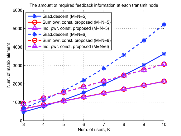
Figure 3: The amount of feedback information at each source node to design precoder

 

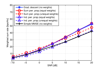
(a) K=4, M=N=5, d=2

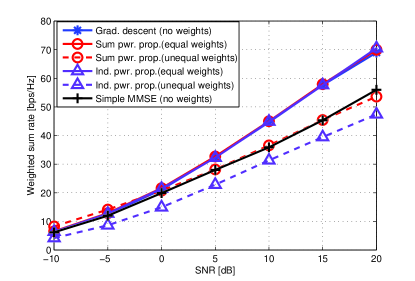
(b) K=5, M=N=6, d=2

Figure 4: The weighted sum rate performance (equal weight $\mu_{k}=1,\forall k$ and unequal weights $\mu_{1}=2,\mu_{k^{\prime}}=0.25,{k^{\prime}}\neq 1$)

 

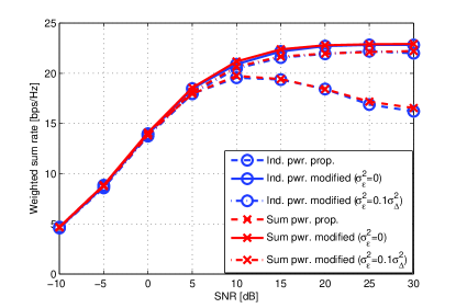
(a) Equal weights ($\mu_{k}=1,\forall k$)

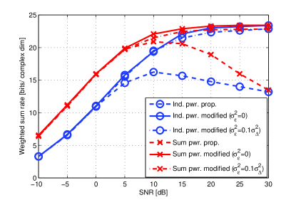
(b) Unequal weights ($\mu_{1}=2,\mu_{k}=0.25,k\neq 1$)

Figure 5: The weighted sum rate performances with imperfect channel state information ($\sigma_{\Delta}^{2}=0.1\times\sigma_{h}^{2},K=4)$

STAGE		Index
Initialization		a.1
	Calculating gradient	a.2
Outer loop	Inner loop: calculating step size	a.3
	Calculating sum rate	a.4
Calculating optimal precoders and decoders		a.5

(a) Description of each stage for gradient descent method

STAGE		Index
Initialization		b.1
	Calculating the variance of noise and interference	b.2
	Calculating the receive filter	b.3
Loop	Calculating the error covariance matrix	b.4
	Calculating the MSE weights	b.5
	Calculating the transmit filter	b.6-1 (for sum power constraint)
	(1-D search is needed for individual power constraint)	b.6-2 (for individual power constraint)
	Calculating sum rate	b.7

(b) Description of each stage for proposed methods

Index	Number of complex multiplication
a.1	$K(M^{2}d+1)+K(K-1)(1+2MNd+N^{2}d)+K(2+2MNd+N^{2}d+N^{3}+c_{N}^{1})$
a.2	$I_{1}\Big{\{}K(2K-1)(1+2MNd+N^{2}d)$
	$+K(2K-1)(9+2c_{N}^{1}+2MN^{2}+2M^{2}N+2M^{2}d+Md^{2})\Big{\}}$
a.3	$I_{1}\Big{\{}KI_{2}(I_{2}+1)/2+KI_{2}\{2K(K-1)(1+2MNd+N^{2}d)$
	$+2K(2+2MNd+N^{2}d+N^{3}+c_{N}^{1})+K(M^{2}d+1)+2+Md^{2}\}\Big{\}}$
a.4	$I_{1}\{K(M^{2}d+1)+K(K-1)(1+2MNd+N^{2}d)+K(2+2MNd+N^{2}d+N^{3}+c_{N}^{1})\}$
a.5	$K(1+2Md+2M^{2}d+c_{Md}^{2})+K(K-1)(2MNd+N^{2}d)$
	$+K(2MNd+2N^{2}d+4Nd^{2}+Md^{2}+d^{3}+c_{N}^{1}+c_{d}^{3}+c_{d}^{2}+c_{dd}^{2})$
b.1	$K(M^{2}d+1)+K(K-1)(1+2MNd+N^{2}d)+K(2+2MNd+N^{2}d+N^{3}+c_{N}^{1})$
b.2	$I_{1}K(K-1)(1+2MNd+N^{2}d)$
b.3	$I_{1}K(3MNd+2N^{2}d+c_{N}^{1})$
b.4	$I_{1}K(2MNd+N^{2}d+Nd^{2}+c_{N}^{1}+c_{d}^{1})$
b.5	$I_{1}Kc_{d}^{1}$
b.6-1	$I_{1}\Big{\{}K(K-1)(2NMd+Md^{2}+M^{2}d)+K(Nd^{2}+d^{3})$
	$+K(3MNd+2Md^{2}+M^{2}d+1+c_{M}^{1})+K(M^{2}d+Md)\Big{\}}$
b.6-2	$I_{1}\Big{\{}K(K-1)(2NMd+Md^{2}+M^{2}d)+I_{3}KM^{2}d$
	$+(I_{3}+1)K(3MNd+2Md^{2}+M^{2}d+1+c_{M}^{1})\Big{\}}$
b.7	$I_{1}\{K(M^{2}d+1)+K(K-1)(1+2MNd+N^{2}d)+K(2+2MNd+N^{2}d+N^{3}+c_{N}^{1})\}$

(c) Number of complex multiplication at each stage

TABLE I: Computational complexity comparison

	Grad. descent method		Prop. method
	Global CSI	Updating coefficients	Local CSI	Updating coefficients
Feedback information	$\{{\bf{H}}_{ij}\}$	$\{{\bf{V}}_{i}\}$, $(i\neq k)$	$\{{\bf{H}}_{ik}\}$	$\{{\bf{U}}_{i}\}$, $\{{\bf{W}}_{i}\}$ (Ind. pwr.)
				$\{{\bf{U}}_{i}\}$, , $\{{\bf{W}}_{i}\}$, $\sum_{i\neq k}\text{Tr}\{{\bf{V}}_{i}{\bf{V}}_{i}^{{}^{\prime}H}\}$ (Sum pwr.)
Matrix size	$MNK^{2}$	$Md(K-1)$	$MNK$	$(Md+d^{2})K$ (Ind. pwr.)
				$(Md+d^{2})K+1$ (Sum. pwr.)
Feedback resource amount	$MNK^{2}$ + $Md(K-1)I_{1}$		$MNK$ + $(Md+d^{2})KI_{1}$ (Ind. pwr.)
			$MNK$ + $((Md+d^{2})K+1)I_{1}$ (Sum. pwr.)

TABLE II: Summary of required feedback information at the $k$-th transmit node, $\textsf{S}_{k}$, $i,j=1\sim K$

References

• [1] K.Β Gomadam, V.Β R. Cadambe, and S.Β A. Jafar, β€œApproaching the capacity of wireless networks through distributed interference alignment,” ArXiv pre-print cs.IT/1011.3816 [ONLINE]. Available:http://arxiv.org/abs/0803.3816.
• [2] H.Β Sung, S.Β H. Park, K.Β J. Lee, and I.Β Lee, β€œLinear precoder designs for K-user interference channels,” IEEE Trans. Wireless Commun., vol.Β 9, pp. 291–301, Jan. 2010.
• [3] S.Β W. Peters and R.Β W. Heath, β€œCooperative algorithms for MIMO interference channels,” IEEE Trans. Veh. Technol., vol.Β 60, pp. 206–218, Jan. 2011.
• [4] V.Β R. Cadambe and S.Β A. Jafar, β€œInterference alignment and degrees of freedom of the K-user interference channel,” IEEE Trans. Inf. Theory, vol.Β 54, pp. 3425–3441, Aug. 2008.
• [5] S.Β S. Christensen, R.Β Agarwal, E.Β Carvalho, and J.Β M. Cioffi, β€œWeighted sum rate maximization using weighted MMSE for MIMO-BC beamforming design,” IEEE Trans. Wireless Commun., vol.Β 7, pp. 4792–4799, Dec. 2008.
• [6] S.Β H. Park, H.Β Park, Y.Β D. Kim, and I.Β Lee, β€œRegularized interference alignment based on weighted sum MSE criterion for MIMO interference channels,” in Proc. IEEE Int. Conf. Communications (ICC), Cape town, South Africa, May 2010.
• [7] D.Β A. Schmidt, S.Β Changxin, R.Β Berry, M.Β L. Honig, and W.Β Utschick, β€œMinimum mean squared error interference alignment,” in 43rd Asilomar conference on signals, systems and computers. ACSSC 2009, CA, USA, Nov. 2009.
• [8] H.Β Shen, B.Β Li, M.Β Tao, and X.Β Wang, β€œMSE-based transceiver designs for the MIMO interference channel,” IEEE Trans. Wireless Commun., vol.Β 11, pp. 3480–3489, Nov. 2010.
• [9] F.Β Negro, S.Β P. Shenoy, I.Β Ghauri, and D.Β T.Β M. Slock, β€œWeighted sum rate maximization in the MIMO interference channel,” in Proc. IEEE. conference on Personal Indoor and Mobile Radio Communications (PIMRC), Istanbul, Turkey, Sept. 2010.
• [10] Q.Β Shi, M.Β Razaviyayn, Z.Β Luo, and C.Β He, β€œAn iteratively weighted MMSE approach to distributed sum-utility maximization for a MIMO interfering broadcast channel,” IEEE Trans. Signal Processing, vol.Β 59, pp. 4331–4340, Sept. 2011.
• [11] G.Β Bresler, D.Β Cartwright, and D.Β Tse, β€œSettling the feasibility of interference alignment for the MIMO interference channel: the symmetric square case,” ArXiv pre-print cs.IT/1104.0888 [ONLINE]. Available:http://arxiv.org/abs/1104.0888.
• [12] R.Β Tresch and M.Β .Guillaud, β€œCellular interference alignment with imperfect channel knowledge,” in Proc. IEEE Int. Conf. Communications (ICC), Dresden, Germany, 2009.
• [13] M.Β B. Shenouda and T.Β N. Davidson, β€œTomlinson-Harashima precoding for broadcast channels with uncertainty,” vol.Β 25, pp. 1380–1389, Sept. 2007.
• [14] G.Β H. Golub and C.Β F.Β V. Loan, Matrix computations.Β Β Β Baltimore, U.S.A.: Johns Hopkins, 1996.
Refer to caption