Diffusion in a logarithmic potential: scaling and selection in the approach to equilibrium

Abstract

The equation which describes a particle diffusing in a logarithmic potential arises in diverse physical problems such as momentum diffusion of atoms in optical traps, condensation processes, and denaturation of DNA molecules. A detailed study of the approach of such systems to equilibrium via a scaling analysis is carried out, revealing three surprising features: (i) the solution is given by two distinct scaling forms, corresponding to a diffusive ($x\sim\sqrt{t}$) and a subdiffusive ($x\ll\sqrt{t}$) length scales, respectively; (ii) the scaling exponents and scaling functions corresponding to both regimes are selected by the initial condition; and (iii) this dependence on the initial condition manifests a “phase transition” from a regime in which the scaling solution depends on the initial condition to a regime in which it is independent of it. The selection mechanism which is found has many similarities to the marginal stability mechanism which has been widely studied in the context of fronts propagating into unstable states. The general scaling forms are presented and their practical and theoretical applications are discussed.

1 Introduction

A large variety of physical problems are governed by the simple diffusion equation which describes a Brownian particle in a logarithmic potential. Such problems range from the momentum spreading of cold atoms in optical traps [1, 2, 3, 4, 5] to the dynamics of “bubbles” in denaturing DNA molecules [6, 7, 8, 9, 10, 11], and from the relaxation of a single particle in a fluid with long-range interactions [12, 13, 14] to models describing brief awakenings in the course of a night’s sleep [15]. In these examples, as well as in others which will be described below, one is interested in the distribution of a fluctuating quantity $x$: for optically trapped cold atoms $x$ stands for the momentum of the atom, in the problem of DNA denaturation $x$ is the length of a denatured unbound loop in the double stranded molecule, and when modeling sleep dynamics, $x$ represents the wakefulness level of a sleeping individual. In the problems we consider, the temporal evolution of the distribution $P(x,t)$ can be approximated when $x$ is large enough by the equation

$$\frac{\partial P(x,t)}{\partial t}=\frac{\partial}{\partial x}\biggl{[}\frac{b}{x}P(x,t)\biggr{]}+\frac{\partial^{2}P(x,t)}{\partial x^{2}}.$$ (1)

The dimensionless parameter $b$, which plays a central role in the solution of the equation, has a different physical meaning in each problem. In physical systems of the type which we consider, Eq. (1) has corrections at small values of $x$, and, in particular, the divergence at small $x$ is not present.

To have a concrete physical picture in mind, we will mostly concentrate on a Brownian particle diffusing under the influence of a one-dimensional external potential which is logarithmic for large $x$:

$$\frac{V(|x|\gg 1)}{k_{B}T}\sim b\log(|x|),$$ (2)

where $T$ is the temperature, $k_{B}$ is Boltzmann’s constant and $b$ measures the strength of the potential. The corresponding Fokker-Planck equation has the form of a continuity equation for the probability distribution

$$\frac{\partial P(x,t)}{\partial t}=-\frac{\partial J(x,t)}{\partial x},\quad\mbox{with}\quad J(x,t)=-V^{\prime}(x)P(x,t)-\frac{\partial P(x,t)}{\partial x},$$ (3)

where $J(x,t)$ denotes the probability current. To simplify notation, here and throughout the paper time is measured in units in which the diffusion coefficient is equal to 1, and the potential is measured in units of temperature, i.e., $k_{B}T=1$. For large values of $|x|$ this Fokker-Planck equation reduces to (1). For some applications it is natural to restrict the variable $x$ to be non-negative, in which case the equation should be supplemented by a boundary condition at $x=0$. We therefore discuss both the case of restricted $x$ with different boundary conditions, and the case where $x$ is unbounded (which requires no additional boundary conditions).

Our goal is to study the long-time behavior of the solutions to this diffusion problem. In a recent paper [16] we have reported that the solutions of equation (3) relax to equilibrium via a universal scaling form which depends on the potential only through its asymptotic form (2), and also depends on the initial condition. In the present paper we elaborate on the analysis of [16], present in more detail the derivation of this result, and discuss its implications and applications.

The scaling form which we find exhibits several features which are not typically found in scaling solutions. (i) For any large finite time, the overall scaling form is comprised of two scaling functions, one corresponding to small values of $x$ ($x\ll\sqrt{t}$) and another corresponding to large values of $x$ ($x\sim\sqrt{t}$). Together, these two scaling functions give the distribution $P(x,t)$ for all values of $x$, including the microscopic scale where the potential deviates from a logarithm. The small-$x$ details of the potential $V(x)$ enter only through the steady-state distribution which multiplies this scaling form. (ii) The equation admits not only one, but a family of such overall scaling forms, each characterized by different scaling exponents. The scaling form which describes the observed relaxation to equilibrium depends on the initial condition via a selection mechanism akin to the marginal stability selection mechanism encountered in, e.g., fronts propagating into unstable states. (iii) As in problems of propagating fronts, by continuously changing the tail of the initial condition, the selected scaling exponent exhibits a “phase transition” from a smoothly varying to a fixed value.

Features (ii) and (iii) of the scaling solution provide an interesting connection between this diffusion problem and the well-known problem of fronts propagating into unstable states. Many systems of the latter type admit a family of traveling-wave solutions with different propagation velocities, and the mechanism by which the eventual velocity and waveform are selected has been widely studied [17]. As described below, the selection mechanism which we find for the diffusion problem is similar in many of its details to that corresponding to propagating fronts. The two problems differ however in some basic aspects: unlike the homogeneous nonlinear propagating front problems, equation (3) is linear yet inhomogeneous in space. Although the inhomogeneity of our problem restricts the utility of mathematical methods used to analyze the selection of front velocities, most notably Fourier analysis, its linearity makes it exactly solvable and facilitates the demonstration of the selection mechanism. The similarities between the problems, suggests that a common mathematical description of their solutions might exist.

As mentioned above, at late times the entire distribution is given by a scaling form (feature (i) above). At late times $t\gg 1$, two different length scales emerge: a large-$x$ length scale of $x\sim t^{1/2}$ and and a small-$x$ length scale of $x\sim t^{\gamma}$ with a $b$-dependent exponent $\gamma<1/2$. Hereafter we refer to these two length scales as “the large-$x$” and “the small-$x$” regions, respectively. The exponent $\gamma$ depends on the boundary conditions, and in particular, for a reflecting boundary condition at the origin, $\gamma=1/(b+1)$. The solution in each of the length scales is given by a different scaling function, with a smooth interpolation between the two functions. Moreover, to leading order in $t$, these two scaling functions yield the solution at any point $x$ (see Fig. 1). Both scaling functions are selected by the initial condition: the large-$x$ scaling function determines the one in the small-$x$ region. In the language of traveling waves, this corresponds to a system with two fronts propagating with different velocities, whereby the selected scaling solution of the “faster front” dictates that of the “slower” one.

For a wide class of initial conditions, which include compactly supported (or “steep”) initial distributions, the large-$x$ scaling solution of Eqs. (2)–(3) has recently been found in [18], [19] and [20]. There, the dependence of the solution on the initial condition and the behavior at small $x$ have not been considered. In fact, in many physical circumstances the initial distribution is not steep. In other situations, the small-$x$ behavior rather than the large-$x$ one determines the physical observables of interest. In these two respects, beyond the relevance of our work to the general theory of selection problems and scaling solutions, it also presents a comprehensive analysis of the scaling solution of (2)–(3) which provides useful results for many concrete systems. To demonstrate the applicability of our results, we consider at the end of this paper three physical examples: (a) cold atoms in an optical lattice undergoing a rapid “quench” from one steady state to another. Here we discuss initial conditions with a fat tail. (b) Nonequilibrium driven models exhibiting real-space condensation. Here we show that current correlations in these systems may be evaluated by considering initial conditions with specific algebraic decay at the tails. (c) The dynamics of loops in DNA molecules undergoing denaturation. Here the effect of an absorbing boundary condition is probed.

The paper is organized as follows. In Sec. 2 we present the scaling solution and its selection mechanism, and heuristically derive its form. The results of this section are backed up by an exact solution of the Fokker-Planck equation (1) which appears in A. In Sec. 3, the scaling solution is discussed in the broader contexts of the general theory of scaling solutions (Sec. 3.1), of selection in problems of propagating fronts (Sec. 3.2), and of the results of previous work on Eq. (1) (Sec. 3.3). The discussion in Sections 2 and 3 is focused on systems whose boundary conditions conserve probability. In Sec. 4 we generalize the results of the previous sections to the case in which probability is not conserved at the boundary. In particular, we show that the large-$|x|$ scaling form is not affected by the boundary conditions. Applications of our results to concrete physical systems are discussed in Sec. 5, in which we also present a general review of some of the problems which are described by Eqs. (2)–(3), for which our results may be relevant. Finally, Sec. 6 contains a summary of our results and some concluding remarks.

2 The scaling solution and its universal character

In this section we present the scaling solution of Eq. (2)–(3). We begin in Sec. 2.1 with a general discussion of the problem of diffusion in a logarithmic potential, and present its scaling solution. In the following subsections this results is derived heuristically, while the exact derivation of this result, which is somewhat technical, is found in A. First, in Sec. 2.3 we demonstrate that in the large-$x$ regime of $x\sim\sqrt{t}$, Eq. (1) admits a one-parameter family of scaling solutions. In Sec. 2.4, we present the selection criterion which explains how the initial conditions determine which member of this family is eventually observed. In Sec. 2.5 we derive the scaling form for the small-$x$ regime. The derivation of Sec. 2.3 rests on the assumption that when $x\sim\sqrt{t}\gg 1$, Eq. (3) can be well approximated by Eq. (1). In Sec. 2.6 we justify this assumption by showing that our scaling solution is universal, i.e., it depends only on the large-$|x|$ tails of the potential (2).

2.1 General discussion of the problem

We begin by writing the Fokker-Planck equation (2)–(3) in more concrete terms. We consider a potential has of form

$$V(x)=b\log(|x|)+U(x),$$ (4)

where the correction $U(x)$ is negligible for large $|x|$ and it ensures that $V(x)$ does not diverge at the origin. For concreteness, we assume that for large $x$

$$U(x\gg 1)=O(|x|^{-\sigma})\quad\mbox{with}\quad\sigma>0.$$ (5)

Regularizing the potential at small $x$ is needed since for $b>1$, the case on which we focus below, a logarithmic divergence of the potential at the origin makes $x=0$ an absorbing state and any normalized initial condition tends to a $\delta$-function distribution around it [21, 22]. This suggests that in systems with $b>1$, physical corrections to the logarithmic potential near the origin cannot be neglected when analyzing the long-time behavior.

With this notation, the Fokker-Planck equation (3) is

$$\frac{\partial P(x,t)}{\partial t}=\frac{\partial}{\partial x}\biggl{[}\frac{b}{x}\bigl{(}1+h(x)\bigr{)}P(x,t)\biggr{]}+\frac{\partial^{2}P(x,t)}{\partial x^{2}}$$ (6)

where

$$h(x)\equiv\frac{xU^{\prime}(x)}{b}=O(|x|^{-\sigma}).$$ (7)

We begin in this section by considering only the boundary condition at $x=0$ where the probability flux at the origin is zero, i.e., $J(0)=0$. This corresponds to diffusion on the entire real line with an even initial condition, or diffusion on the positive half line with a reflecting boundary condition at the origin. The general case, and the effect of other boundary conditions will be examined in Sec. 4.

The stationary solution of the diffusion equation (3) in this potential has the form of a Boltzmann distribution

$$P^{*}(x)=\frac{1}{Z}e^{-V(x)}\sim\frac{1}{Z}x^{-b},$$ (8)

where $Z$ is a normalization constant given by $Z=\int e^{-V(x)}dx$. For $b>1$, $Z$ is finite and the system tends towards this unique equilibrium distribution regardless of the initial condition (we assume that the potential does not contain infinite energy barriers and the system is ergodic). However, for $b\leq 1$, the equilibrium distribution cannot be normalized. In this case, any normalized initial condition tends to zero. Thus, potentials with logarithmic tails are a marginal case for the diffusion equation. Any potential which increases at large $x$ faster than a logarithm “traps” the particle and the probability distribution reaches a steady state at long times. On the other hand, potentials which increase with $x$ slower than logarithmically are non-trapping and the probability distribution eventually spreads out to infinity. In the marginal case where the potential is logarithmic at large $x$, the particle is trapped at low temperatures and becomes delocalized at high temperatures, as the dimensionless parameter $b$ changes from $b>1$ to $b\leq 1$.

The aim of this paper is to describe how $P(x,t)$ relaxes towards the eventual Boltzmann distribution. We therefore concentrate on the normalizable case $b>1$. Recently, [18, 19, 20] have shown that this relaxation is given by a useful and compact scaling form. The scaling form which was found, however, describes the solution of Eqs. (2)–(3) only for a specific (albeit large) class of initial conditions, and it represents correctly only the large-$|x|$ behavior of the actual scaling solution. The main result of the present work is the surprising fact that the long-time scaling form of the solution depends on the initial condition in a non-trivial fashion. Moreover, the entire solution can be described by a scaling form, where the non-universal features are contained in $P^{*}(x)$. We now present these results, and then derive them.

As we are interested in the relaxation towards the equilibrium distribution, it is convenient to study the deviation of $P(x,t)$ from $P^{*}(x)$. To this end we define a function $G(x,t)$ via

$$\qquad P(x,t)=P^{*}(x)\bigl{[}1+G(x,t)\bigr{]},\quad\mbox{or equivalently}\quad G(x,t)=\frac{P(x,t)-P^{*}(x)}{P^{*}(x)}.$$ (9)

We seek scaling solutions of $P(x,t)-P^{*}(x)$, or equivalently of $G(x,t)$, rather than of $P(x,t)$. Note that since the Fokker-Planck equation is linear and it is satisfied by $P^{*}(x)$, the distribution $P(x,t)$ and the deviation from equilibrium $P(x,t)-P^{*}(x)=P^{*}(x)G(x,t)$ satisfy the same equation. However, while $\int P(x,t)dx=1$, here $\int P^{*}(x)G(x,t)dx=0$. Looking for a scaling form for solutions with zero normalization is our primary extension of the calculations of [18, 19, 20] which enables us to find all scaling solutions to the problem.

2.2 The scaling solution

The Fokker-Planck equation (1) can be solved exactly by standard methods [23]. By a transformation of variables, it can be mapped to a Schrödinger equation in imaginary time which describes a quantum particle moving in an inverse square potential. Analysis of this quantum problem yields the exact solution of the equation for arbitrary initial conditions represented as a series of Bessel functions. Asymptotic analysis of these Bessel functions allows one to identify the scaling form which characterizes the approach to equilibrium at late times. Although this calculation is straightforward, it is rather technical and lengthy. We therefore delay its presentation to A. Here, we present the results of this calculation, and in the rest of this section we heuristically motivate these results.

According to the exact calculation of A, the long-time behavior of the solution of the Fokker-Planck equation (3) with any normalizable initial condition and for a reflecting boundary condition at the origin, is given, to leading order in $t$, by

$$P(x,t)\approx P^{*}(x)+CP^{*}(x)\cdot\left\{\begin{array}[]{ll}g_{\beta}\bigl{(}\frac{|x|}{t^{1/(b+1)}}\bigr{)}t^{-\delta}&\mbox{ for }|x|\leq x_{1}(t)\\ \\ f_{\beta}\bigl{(}\frac{|x|}{t^{1/2}}\bigr{)}t^{-\beta}&\mbox{ for }|x|\geq x_{1}(t)\end{array}\right.,$$ (10)

where $x_{1}(t)$ can be chosen to have any value which satisfies

$$t^{1/(b+1)}\ll x_{1}(t)\ll t^{1/2},$$ (11)

and the scaling functions are given by

$$g_{\beta}(z) =-{\textstyle\frac{4(b+1)}{rZ(2\beta+b-1)}}+z^{b+1},$$ (12)

$$f_{\beta}(u) =u^{b+1}\,_{1}\!F_{1}\Bigl{(}{\textstyle\frac{1+b+2\beta}{2}};{\textstyle\frac{b+3}{2}};{\textstyle-\frac{u^{2}}{4}}\Bigr{)}.$$ (13)

The values of the scaling exponents $\beta$ and $\delta$ and of the constant $C$ will be discussed shortly. The constant $r$ depends on the domain on which the diffusion is defined: $r=2$ for diffusion on the positive half-line (with a wall at the origin), while $r=1$ for symmetric diffusion on the entire real line. Here, ${}_{1}F_{1}$ is the confluent hypergeometric function, whose known properties yield the asymptotic form [24]

$$f_{\beta}(u)\sim\left\{\begin{array}[]{ll}u^{b+1}\phantom{e^{-\frac{u^{2}}{4}}}&\mbox{ for }u\ll 1\\ Du^{-2\beta}\phantom{e^{-\frac{u^{2}}{4}}}&\mbox{ for }u\gg 1,\beta<1\\ u^{b+1}e^{-\frac{u^{2}}{4}}&\mbox{ for }u\gg 1,\beta=1\end{array}\right.,$$ (14)

where $D=\frac{2^{1+b+2\beta}\Gamma[(b+3)/2]}{\Gamma(\beta-1)}$.

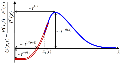
Figure 1: A schematic representation of the solution $P(x,t)$ (Eq. (10)) at a given late time $t\gg 1$ (not drawn to scale). The red double line represents the small-$x$ scaling form $g_{\beta}(x/t^{1/(b+1)})t^{-\delta}$ while the blue solid line represents the large-$x$ scaling form $f_{\beta}(x/t^{1/2})t^{-\beta}$. The interval on which the two solutions overlap (Eq. (11)) is labeled $x_{1}(t)$.

The solution (10) is presented schematically in Fig. 1. It is made up of two different scaling forms with different dynamical exponents: $x\sim t^{1/(b+1)}$ and $x\sim t^{1/2}$. At small values of $|x|$, the solution is flat up to $x\sim t^{1/(b+1)}$, with a value that approaches zero as $t^{-\delta}$. At large values of $|x|$, the solution exhibits a peak at $x\sim\sqrt{t}$, whose height shrinks as $t^{-\beta}$ (this schematic form is modified for negative $\beta$ since in this case $f_{\beta}(u)$ diverges for large $u$, see (14)). As Eqs. (12)–(14) indicate, the two scaling functions are, to leading order in $t$, identical for any $x_{1}(t)$ in the range (11), explaining why the crossover point between the two regimes can be chosen anywhere in this range.

According to the calculation of A, the values of $\beta$, $\delta$ and $C$ depend of the initial conditions. We consider initial conditions $G_{0}(x)\equiv G(x,0)$ which for large $|x|$ have an asymptotic form

$$G_{0}(|x|\gg 1)\sim A|x|^{-a}.$$ (15)

Here, $a>1-b$ must hold for $P(x,0)$ to be normalizable. Note that $a$ may be negative. If $G_{0}(x)$ decays faster than a power law, we formally take $a=\infty$. A few examples of different initial conditions and the corresponding values of $a$ and $A$ are given in Table 1. In Sec. 4 we briefly discuss cases in which $G_{0}(x)$ is not asymptotically symmetric, i.e., when the tails of $G_{0}(x)$ at $x\to\pm\infty$ decay at different rates.

$P(x,0)\quad{}$	$G_{0}(x)$		$\;a{}$	$\;A{}$
$\delta(x-x_{0})\quad{}$	$\frac{\delta(x-x_{0})}{P^{*}(x)}-1$$\;\sim\;{}$	$-1\quad{}$	$0$	$-1$
$Ce^{-|x|/x_{0}}\quad{}$	$\frac{Ce^{-|x|/x_{0}}}{P^{*}(x)}-1$$\;\sim\;{}$	$-1\quad{}$	$0$	$-1$
$C|x|^{-(b+1)}+\ell(x)\quad{}$	$\frac{C|x|^{-(b+1)}+\ell(x)}{P^{*}(x)}-1$$\;\sim\;{}$	$-1\quad{}$	$0$	$-1$
$C|x|^{-(b-1)}+\ell(x)\quad{}$	$\frac{C|x|^{-(b-1)}+\ell(x)}{P^{*}(x)}-1$$\;\sim\;{}$	$CZ|x|^{+1}\quad{}$	$-1$	$CZ$
$P^{*}(x)+C|x|^{-(b+1)}+\ell(x)\quad{}$	$\frac{C|x|^{-(b+1)}+\ell(x)}{P^{*}(x)}\phantom{{}-1}$$\;\sim\;{}$	$CZ|x|^{-1}\quad{}$	$1$	$CZ$
$P^{*}\bigl{(}|x|+x_{0}\bigr{)}+\ell(x)\quad{}$	$\frac{P^{*}(|x|+x_{0})+\ell(x)}{P^{*}(x)}-1$$\;\sim\;{}$	$-bx_{0}|x|^{-1}\quad{}$	$1$	$-bx_{0}$
$P^{*}(x)\bigl{[}1+e^{-|x|/x_{0}}\bigr{]}+\ell(x)\quad{}$	$e^{-|x|/x_{0}}+\frac{\ell(x)}{P^{*}(x)}$$\;\sim\;{}$	$e^{-|x|/x_{0}}\quad{}$	$\infty$
$CP^{*}(x)\bigl{[}1+e^{-|x|/x_{0}}\bigr{]}\quad{}$	$C-1+Ce^{-|x|/x_{0}}$$\;\sim\;{}$	$C-1\quad{}$	$0$	$C-1$

Table 1: A variety of initial conditions $P(x,0)$ and the corresponding values of $a$ and $A$ according to Eq. (15). $G_{0}(x)\equiv G(x,0)$ is defined by Eq. (9), and its leading asymptotic behavior for $|x|\gg 1$ is presented. $\ell(x)$ and $C$ are a compactly-supported function and a constant whose values change from line to line. They are added to ensure the normalization $\int P(x,0)dx=1$. The equilibrium distribution $P^{*}(x)$ is given in Eq. (8).

For this large class of initial conditions, the scaling exponents are given by

$$\beta=\beta(a)=\left\{\begin{array}[]{ll}\frac{a}{2}&\mbox{if }a<2\\ 1&\mbox{if }a>2\end{array}\right.$$ (16)

and

$$\delta=\delta(a)=\beta(a)+\frac{b-1}{2}$$ (17)

For $a<2$, the constant $C$ is

$$C=\frac{\Gamma(1-\frac{a}{2})}{2^{b+a+1}\Gamma(\frac{3+b}{2})}\cdot A,$$ (18)

while for $a>2$, $C$ depends on the full forms of the initial condition and the potential. For $a=2$ there are logarithmic corrections to Eq. (10), which are presented in Eqs. (117), (118) and (121) of A.

We make two comments about the solution (10). First, we would like to emphasize the non-trivial fashion in which the solution depends on the initial condition. The scaling functions $f_{\beta}$ and $g_{\beta}$ and the scaling exponent $\delta$ are determined by the value of $\beta$. The $\beta$ exponent exhibits a “phase transition” at $a=2$, between a regime ($a<2$) in which $\beta$ depends on the value of $a$ and a regime ($a>2$) in which it does not. As discussed in Sec. 2.4 below, it is this threshold phenomenon which ties our scaling solution with the problem of velocity selection of propagating fronts.

The second comment is that this scaling solution is universal, in two ways: it is independent of the small-$x$ details of the potential, i.e., of $U(x)$ of Eq. (4). It is also independent of the small-$x$ details of the initial condition. When we say below that a particular result is universal, we use the term in both these meanings. To be more precise, the universal function is $\frac{P(x,t)-P^{*}(x)}{P^{*}(x)}$; $P(x,t)$ itself depends on $U(x)$ for small values of $x$, but only through the simple Boltzmann distribution (8). It is interesting to note that when $a>2$, where the solution does not depend on the initial condition, the constant $C$ is non-universal, while in the case of $a\leq 2$, where the initial condition does affect the scaling form, $C$ is universal.

In the remainder of this section, we motivate these results in order to gain an understanding of their origin. To do so, we derive these results in a heuristic fashion which, although not rigorous, is more transparent than the calculation of A. In this heuristic derivation, we do not presume the results of A, but for a single fact: in order to establish the selection mechanism which leads to Eq. (16) (in Sec. 2.4), we rely on the fact that localized initial conditions $G_{0}(x)$ (which correspond to $a=\infty$) evolve into scaling solutions of the form (10) with $\beta=1$. In other words, using the scaling solution for localized initial conditions, we are able to find the scaling solution for all initial conditions.

2.3 Scaling solution for $|x|\sim\sqrt{t}$ (“large $x$”)

As we are seeking a scaling form for $G(x,t)$ (Eq. (9)) rather than for $P(x,t)$, we start by writing down the equation governing the evolution of $G$. Substituting (9) in the Fokker-Planck equation (6) we find

$$\frac{\partial G}{\partial t}=-V^{\prime}(x)\frac{\partial G}{\partial x}+\frac{\partial^{2}G}{\partial x^{2}}=-\frac{b}{x}\bigl{(}1+h(x)\bigr{)}\frac{\partial G}{\partial x}+\frac{\partial^{2}G}{\partial x^{2}}.$$ (19)

Here we have used Eq. (8) to deduce that $\frac{\partial P^{*}(x)}{\partial x}=-V^{\prime}(x)P^{*}(x)$. Our heuristic derivation of the scaling solution (10) proceeds by dropping the $h(x)$ term in this equation, which is negligible for large values of $x$. This leads to

$$\frac{\partial G(x,t)}{\partial t}=-\frac{b}{x}\frac{\partial G(x,t)}{\partial x}+\frac{\partial^{2}G(x,t)}{\partial x^{2}},$$ (20)

which is equivalent to Eq. (1). Dropping $h(x)$ is justified below, in Sec. 2.6, where we establish the universality of the results which we now derive, i.e., their independence of the form of $h(x)$.

The goal of the present subsection is to show that Eq. (20) admits a family of scaling solutions. We start by looking for scaling solutions of the form

$$G(x,t)=t^{-\beta}{f}\Bigl{(}\frac{|x|}{\sqrt{t}}\Bigr{)}$$ (21)

where the scaling exponent $\beta$ and the function $f(u)$ are to be determined. This corresponds to the ansatz

$$P(x,t)=P^{*}(x)+P^{*}(x)t^{-\beta}{f}\Bigl{(}\frac{|x|}{\sqrt{t}}\Bigr{)}\sim|x|^{-b}\Bigl{[}1+t^{-\beta}f\Bigl{(}\frac{|x|}{\sqrt{t}}\Bigr{)}\Bigr{]}$$ (22)

for the probability distribution. Substituting (21) in the Fokker-Planck equation (20) yields a family of ordinary differential equations for $f(u)$,

$$f^{\prime\prime}+\Bigl{(}\frac{u}{2}-\frac{b}{u}\Bigr{)}f^{\prime}+\beta f=0$$ (23)

with $\beta$ a free parameter. For every value of $\beta$ this equation has a solution

$$f(u)=C_{1}u^{b+1}\,_{1}\!F_{1}\left(\frac{1+b+2\beta}{2};\frac{b+3}{2};-\frac{u^{2}}{4}\right)+C_{2}\,{}_{1}\!F_{1}\left(\beta;\frac{1-b}{2};-\frac{u^{2}}{4}\right),$$

where ${}_{1}F_{1}$ is the confluent hypergeometric function [24], and $C_{1}$ and $C_{2}$ are integration constants. The three unknown constants $\beta$, $C_{1}$ and $C_{2}$ should in principle be determined by the two boundary conditions at $u=0$ and $u=\infty$ and by the initial condition.

The study of the small-$x$ scaling solution in Sec. 2.5 below shows that the proper boundary condition to consider at $u=0$ is

$$f(u\ll 1)\sim u^{b+1}.$$ (25)

Using the asymptotics of the hypergeometric function [24]

$$\qquad_{1}F_{1}\bigl{(}r;s;{\textstyle-\frac{u^{2}}{4}}\bigr{)}=\left\{\begin{array}[]{ll}1+O(u^{2})&\mbox{ for }u\ll 1\\ \frac{4^{r}\Gamma(s)+O(u^{-2})}{\Gamma(s-r)}\cdot u^{-2r}\phantom{e^{-\frac{u^{2}}{4}}}&\mbox{ for }u\gg 1,\,r-s\neq 0,1,2,\ldots\\ \frac{\Gamma(s)+O(u^{-2})}{(-4)^{r-s}\Gamma(r)}\cdot u^{2(r-s)}e^{-\frac{u^{2}}{4}}&\mbox{ for }u\gg 1,\,r-s=0,1,2,\ldots\end{array}\right.,$$ (26)

we see that the boundary condition (25) implies that $C_{2}=0$, and therefore $f(u)=Cf_{\beta}(u)$, where $f_{\beta}$ is given in (13), and we have defined $C\equiv C_{1}$.

Without another condition which may set the values of the two remaining constants, $C$ and, more importantly, $\beta$, we are still left with a family of scaling solutions. Note that the conservation of probability cannot be used to determine these constants, since the scaling ansatz (21) does not hold for small enough values of $x$. Similarly, the known stationary distribution (8) does not provide a boundary condition as all solutions relax to it (as can be seen using (26)). We therefore arrive at the uncommon (although not unique, see [25]) situation in which the scaling exponent $\beta$ and the scaling function $f$ are determined by the initial condition. This situation confronts us with a problem of selection: which of the family of scaling solutions is selected by the initial condition of the physical system under consideration? We turn to this question in the next subsection.

2.4 Stability and the selection of the scaling solution

In this section we elucidate the selection mechanism which leads to Eq. (16). Since probability is locally conserved by the diffusion equation (3), it is reasonable to expect that the relaxation towards equilibrium propagates as a diffusive “front” from the origin towards the tails. If this is so, then at any given time, the tails of $G(x,t)$ do not yet “feel” this front, and they should therefore be given by the initial distribution. By matching the tails of Eq. (2.3) with initial conditions of the form (15), the asymptotics (26) of the hypergeometric function suggest that $\beta(a)=a/2$ and $C$ is given by (18) when $a\neq 2,4,6,\ldots$.

According to the exact calculation of A, the naive argument of the previous paragraph is correct only for $a<2$. To understand why the argument fails when $a>2$, we turn to a stability analysis of the scaling solutions and show that those with $\beta>1$ are unstable to localized perturbations. To this end, we make use of the following result which is derived in A: localized initial conditions $G(x,0)$, such as compactly supported ones, evolve at long times to

$$G(x,t)\sim t^{-1}f_{1}\Bigl{(}\frac{x}{\sqrt{t}}\Bigr{)}$$ (27)

where $f_{1}(u)$ is given in (13). This result can heuristically be understood as follows: if the initial condition is compactly supported, then it is plausible that the selected solution will be the one whose decay at the tails is steepest. The asymptotics (26) of the scaling solutions show that this is the $\beta=1$ scaling function. We note that using the identity

$$\,_{1}\!F_{1}(A;A;z)=e^{z},$$ (28)

one can simplify the expression for the scaling function to $f_{1}(u)=u^{b+1}e^{-{u^{2}}/{4}}$.

Let us consider a distribution which at some time $t$ is close to a scaling solution of the form (22). The distribution cannot be exactly equal to this scaling solution in any physical situation: at small enough $x$’s, where the potential deviates from a logarithm, the scaling form breaks down. At best, the exact solution is equal to the scaling solution plus a small localized disturbance $\delta P$, i.e.,

$$P(x,t)-P^{*}(x)=CP^{*}(x)t^{-\beta}f_{\beta}\Bigl{(}\frac{x}{\sqrt{t}}\Bigr{)}+\delta P(x,t)$$ (29)

Examining Eq. (29) we see that the late-time behavior of the solution will be close to the scaling solution $f_{\beta}$ if the disturbance $\delta P$ is negligible compared to it. In other words, at late times we can only see scaling solutions which are stable with respect to local perturbations. In order to ascertain the stability of the different scaling solutions, we should examine how localized perturbations around them evolve in time. Since the Fokker-Planck equation is linear, the evolution of such localized perturbations is independent of that of the scaling solution. This simplifies the stability analysis: we need only to solve the Fokker-Planck equation for localized initial conditions.

We now use the result (27) from the exact calculation, and find that at late times, Eq. (29) evolves to

$$P^{*}(x)t^{-\beta}f_{\beta}C\Bigl{(}\frac{x}{\sqrt{t}}\Bigr{)}+\delta P(x,t)\approx P^{*}(x)\Bigl{[}Ct^{-\beta}f_{\beta}\Bigl{(}\frac{x}{\sqrt{t}}\Bigr{)}+\tilde{C}t^{-1}f_{1}\Bigl{(}\frac{x}{\sqrt{t}}\Bigr{)}\Bigr{]}.$$ (30)

When $\beta<1$ the second term on the rhs is negligible compared to the first, and the scaling solution is stable to localized perturbations. On the other hand, when $\beta>1$ the second term dominates the late time behavior. Such scaling solutions are unstable and can never be observed in physical systems. We thus see that initial conditions of the form (15) with $a<2$, which “excite” scaling solutions $f_{\beta}$ with $\beta<1$, evolve to a scaling solution which depends on $a$. “Most” initial conditions, however, evolve towards the marginally stable scaling solution of $\beta=1$. By “most” we mean that the basin of attraction of the $\beta=1$ solution in the space of all initial conditions has a higher dimension than the basins of attraction of solutions with any $\beta<1$. Note that when $a>2$, the constant $\tilde{C}$ is determined by the localized perturbation rather than the tail of the initial condition, and therefore it is not given by Eq. (18).

2.5 Scaling solution for $|x|\ll\sqrt{t}$ (“small $x$”)

In this section we show that when $|x|\ll\sqrt{t}$, the probability $P(x,t)$ is also given in the long time limit by a scaling form. This scaling form is different from the one discussed above, but it, too, depends on the initial condition. Surprisingly, this scaling form is universal: it depends on the full details of the potential $V(x)$ only through the stationary distribution (8) which multiplies the scaling function.

Unlike the large-$x$ scaling form, the small-$x$ scaling form depends on the boundary condition at the origin. As mentioned above, we assume in this section that the probability current at the origin (defined in Eq. (3)) vanishes at all times: $J(0,t)=0$. This boundary condition translates into

$$\frac{\partial G}{\partial x}\biggr{|}_{x=0,t}=0$$ (31)

as long as $P^{*}(0)\neq 0$. The results for other boundary conditions are discussed in Sec. 4.

From the calculation of Sec. 2.3 we already know that at $x$’s which scale as $\sqrt{t}$, $G(x,t)$ is given by (21) and (13) with $\beta$ which depends on the initial condition. We now examine the solution at $x$ which scale as $t^{-\gamma}$, with $0\leq\gamma<\frac{1}{2}$. To this end, we look for scaling solutions of the form

$$G(x,t)=t^{-\delta_{\gamma}}g_{\gamma}\Bigl{(}\frac{x}{t^{\gamma}}\Bigr{)},$$ (32)

which we call “the solution at scale $t^{\gamma}$”.

We begin by considering the unscaled solution $G(x,t)$ itself (this is the case $\gamma=0$). Substituting the ansatz

$$G(x,t)=t^{-\delta_{0}}g_{0}(x),$$ (33)

in the Fokker-Planck equation (19) yields

$$g_{0}^{\prime\prime}(x)-V^{\prime}(x)g_{0}^{\prime}(x)=-\delta_{0}t^{-1}g_{0}(x).$$ (34)

For $t\gg 1$ the term on the rhs becomes negligible. We thus arrive at the simple equation $g_{0}^{\prime\prime}(x)-V^{\prime}(x)g_{0}^{\prime}(x)=0$ which can be integrated, yielding

$$g_{0}(x)=C_{3}+C_{4}\int_{0}^{x}e^{V(y)}dy,$$ (35)

where $C_{3}$ and $C_{4}$ are integration constants. The boundary condition (31) implies that $g_{0}^{\prime}(0)=0$, which means that $C_{4}=0$. Therefore, for values of $x$ which are small enough, $G(x,t)=C_{3}t^{-\delta_{0}}$.

We now proceed to examine the solution at scales $t^{\gamma}$ with $0<\gamma<\frac{1}{2}$. At late times, $x\sim t^{\gamma}\gg 1$, and we can replace $V(x)\approx b\log x$. Substituting the ansatz (32) in the equation (20) yields the ordinary differential equation in the scaling variable $z=xt^{-\gamma}$

$$g_{\gamma}^{\prime\prime}(z)-\frac{b}{z}g_{\gamma}^{\prime}(z)=-[\gamma zg_{\gamma}^{\prime}(z)+\delta_{\gamma}g_{\gamma}(z)]t^{-(1-2\gamma)}.$$ (36)

As before, we assume that the two terms which are proportional to $t^{-(1-2\gamma)}$ are negligible at large times and we drop them. The validity of this assumption will be examined below. We are left with the equation:

$$g_{\gamma}^{\prime\prime}(z)-\frac{b}{z}g_{\gamma}^{\prime}(z)=0,$$ (37)

whose solution is given by

$$g_{\gamma}(z)=C_{5}+C_{6}z^{b+1}.$$ (38)

The picture that emerges is that at every scale $t^{\gamma}$ the solution is either a constant $C_{5}$ or a power law $C_{6}z^{b+1}$. At a single intermediate scale, both $C_{5}\neq 0$ and $C_{6}\neq 0$. Continuity at small $x$ implies that if $C_{5}\neq 0$ then $C_{5}=C_{3}$. With an abuse of notation, we shall from now on denote the exponent of this special intermediate scale by $\gamma$. At this intermediate scale, we expect the solution for large values of $z$ to coincide with the small $u$ behavior of the solution in the $x\sim\sqrt{t}$ region (see Eqs. (10)–(16)). This yields the condition (25). Using $G(ut^{1/2},t)\approx Ct^{-\beta(a)}u^{b+1}$ (see (14)), we find that $C_{6}=C$, and

$$\delta_{\gamma}(a)=\beta(a)+(b+1)({\textstyle\frac{1}{2}}-\gamma).$$ (39)

We note that for the scaling solution (38), the two terms that were neglected when passing from Eq. (36) to (37) are indeed negligible as long as $z\ll t^{\frac{1}{2}-\gamma}$, or equivalently $x\ll t^{\frac{1}{2}}$.

We are now left with the problem of ascertaining the values of the two remaining undetermined constants $\gamma$ and $C_{3}$. These can be found with the help of the conservation of probability (we once again make use of the boundary condition (31)). Choosing $t^{\gamma}\ll x_{1}(t)\ll t^{1/2}$, we can write

$$0=\int_{0}^{\infty}\bigl{[}P(x,t)-P^{*}(x)\bigr{]}dx=\int_{0}^{\infty}P^{*}(x)G(x,t)dx=I_{1}(t)+I_{2}(t),$$ (40)

where we have defined

$$I_{1}(t) \equiv\int_{0}^{x_{1}(t)}P^{*}(x)G(x,t)dx\approx t^{-\delta_{\gamma}}\int_{0}^{x_{1}(t)}P^{*}(x)\bigl{[}C_{3}+Cx^{b+1}t^{-\gamma(b+1)}\bigr{]}dx,$$

$$I_{2}(t) \equiv\int_{x_{1}(t)}^{\infty}P^{*}(x)G(x,t)dx\approx t^{-\beta}\int_{x_{1}(t)}^{\infty}\frac{C}{Z}x^{-b}f_{\beta}\Bigl{(}\frac{x}{\sqrt{t}}\Bigr{)}dx.$$ (41)

In these equations we have substituted the small-$x$ and large-$x$ scaling solutions for $G$. To leading order in $t$, Eq. (40) gives $C_{3}t^{-\delta_{\gamma}}=-\frac{2C}{rZ}\int_{0}^{\infty}u^{-b}f_{\beta}(u)du\,t^{-\beta-(b-1)/2}$, where

$$r=2\int_{0}^{\infty}P^{*}(x)dx=\left\{\begin{array}[]{ll}2&\mbox{for diffusion on positive half-line}\\ 1&\mbox{for diffusion on entire real line}\end{array}\right..$$ (42)

Using (39) we deduce that

$$\gamma=\frac{1}{b+1}$$ (43)

and

$$C_{3}=-\frac{2C}{rZ}\int_{0}^{\infty}u^{-b}f_{\beta}(u)du=-\frac{C}{rZ}\cdot\frac{4(b+1)}{2\beta(a)+b-1}.$$ (44)

To sum up, we see that for any $x_{1}(t)$ in the range (11),

$$G(|x|\leq x_{1}(t),t)\approx Ct^{-\beta-\frac{b-1}{2}}g_{\beta}\bigg{(}\frac{|x|}{t^{1/(b+1)}}\biggr{)},$$ (45)

where

$$g_{\beta}(z)=-{\textstyle\frac{4(b+1)}{rZ(2\beta+b-1)}}+z^{b+1}.$$ (46)

Once again we find a scaling solution which depends on (the tails of) the initial condition. On the other hand, just like the scaling solution at large-$x$, this solution is essentially independent of the full details of the potential $V(x)$, which only serves to determine the stationary solution $P^{*}(x)$ and, when $a>2,$ the constant $C$.

We emphasize that the analysis presented above holds for all $|x|<x_{1}(t)$, including the region around the origin where the potential is not logarithmic. For any fixed $x$ (which does not scale with $t$), Eqs. (45) and (46) agree with rigorous results obtained for discrete random walks in a logarithmic potential [26, 27].

2.6 Universality of late-time scaling solutions

In this section, we establish the universality of the results of Sec. 2.3. That is, we show that they depend only on the logarithmic tail of the potential, and not on the $h(x)$ correction term of Eqs. (7) and (19). Moreover, our argument demonstrates that the details of the initial condition near the origin are also irrelevant for the large-$x$ scaling form.

To establish the required universality, we rescale $x$, $t$ and $G(x,t)$ by defining a rescaled function

$$G_{\Lambda}(x,t)\equiv\Lambda^{2\beta}G(\Lambda x,\Lambda^{2}t).$$ (47)

Thus, up to a normalization factor which depends on $\beta$, the rescaled function $G_{\Lambda}(x,t)$ is equal to $G$ at time $\Lambda^{2}t$ as seen at the spatial scale $\Lambda x$. The equation for the evolution of $G_{\Lambda}$ may be straightforwardly obtained by substituting the definition (47) into Eq. (19), yielding

$$\frac{\partial G_{\Lambda}(x,t)}{\partial t}=-\frac{b}{x}\bigl{(}1+h_{\Lambda}(x)\bigr{)}\frac{\partial G_{\Lambda}(x,t)}{\partial x}+\frac{\partial^{2}G_{\Lambda}(x,t)}{\partial x^{2}},$$ (48)

where $h_{\Lambda}(x)\equiv h(\Lambda x)$.

The solution $G(x,t)$ at a given late time $t\gg 1$ can be obtained in two ways: either by propagating the initial condition according to Eq. (19), or by rescaling the initial condition, propagating it according to Eq. (48) to (rescaled) time 1 and rescaling back. In the second way, the correction $h(x)$ is negligibly small. According to this procedure, we obtain the scaling limit by replacing $\Lambda$ with $\sqrt{t}$:

$$t^{\beta}G(ut^{1/2},t)=G_{\sqrt{t}}(u,1)\underset{t\to\infty}{\longrightarrow}G_{\infty}(u,1)\equiv{f}(u).$$ (49)

The exponent $\beta$ must be chosen appropriately so that the $t\to\infty$ limit exists and is not zero. The limiting function $G_{\infty}(x,t)$ evolves according to (48) with

$$h_{\infty}(x)=\lim_{\Lambda\to\infty}h_{\Lambda}(x)\sim\lim_{\Lambda\to\infty}(\Lambda x)^{-\sigma}=0$$ (50)

for any $x\neq 0$, see (7). Therefore, the scaling limit of the original Fokker-Planck equation does not depend on $h(x)$.

The initial condition for the rescaled problem (48) is

$$G_{\infty}(x,0)\equiv\lim_{\Lambda\to\infty}G_{\Lambda}(x,0)=\lim_{\Lambda\to\infty}\Lambda^{2\beta}G(\Lambda x,0).$$ (51)

This limiting initial condition $G_{\infty}(x,0)$ is in many cases a singular function, similar to the Dirac $\delta$-function but with a different type of singularity. If the tails of $G(x,0)$ at $x\to\pm\infty$ decay with $|x|$ faster than algebraically (e.g., exponentially), then $G_{\infty}(x,0)$ is zero when $x\neq 0$ and is singular at the origin. The exact details of the initial condition around the origin are lost in the limit which yields $G_{\infty}(x,0)$. The tails of the initial condition may, however, affect $G_{\infty}$: an initial condition which decays algebraically as in Eq. (15) is rescaled to $G_{\Lambda}(x,0)\sim\Lambda^{2\beta-a}A|x|^{-a}$. If $\beta=a/2$, the rescaled initial condition $G_{\infty}$ has the same algebraic decay as $G$. We see that initial conditions may affect the scaling solution only through their tails, and that for initial conditions with power-law tails, a limit of (51) exists only when choosing $\beta\leq a/2$ (compare with (16)).

The rescaling argument which we have presented in this section is inspired by the renormalization group (RG) techniques used by Goldenfeld et al. [28] and by Bricmont and Kupiainen [29] to analyze nonlinear partial differential equations. Here we have used their method to analyze a linear equation which is inhomogeneous in space. From the RG perspective, the rescaling transformation (47) can be viewed as an RG transformation that has a one-parameter family of fixed points $f_{\beta}(u)$. The scaling limit of the original equation is determined by the appropriate fixed point, which is not affected by the addition of $h(x)$. Therefore, the $h(x)$ term in the equation is irrelevant and the scaling solution is universal in the RG sense.

3 Comments on the scaling solution

In this section we comment on the scaling solution derived above and discuss it in some broader contexts.

3.1 The scaling solution and incomplete self-similarity

The dependence of the scaling exponent $\beta$ on the initial condition signals the failure of dimensional analysis. The latter is easily seen to predict incorrectly that $\beta=\frac{1-b}{2}$. The reason for this failure is the following. The prediction of dimensional analysis for the diffusion equation rests crucially on the conservation of probability [25]. When $b>1$, the limiting rescaled equation (1) does not conserve probability at the origin because of the singularity of the potential there [21, 22]. It is the $U(x)$ term in the potential (4) which guarantees conservation of probability, and rescaling it away (as was done in Sec. 2.6) yields a singular limit. In practice, this means that at any finite time $t$, no matter how late, corrections due to the potential $U(x)$ inevitably affect the form of the solution at small enough values of $x$. The scaling form (22), in which these corrections are not taken into account, should not be expected to conserve probability by itself, and therefore, the scaling exponent $\beta$ cannot be found by dimensional analysis. In the terminology of Barenblatt, the scaling solution to our problem exhibits self-similarity of the second kind (see [25]).

It is interesting to note that when $b\leq 1$, the solution of the diffusion equation (2)–(3) approaches a self-similar solution of the first kind, i.e., one whose scaling exponents can be determined by dimensional analysis. The scaling solution in this case was found in [19, 20]. Since there is no equilibrium distribution when $b\leq 1$, one cannot define $G(x,t)$ according to Eq. (9). Nonetheless, one may look for scaling solutions of the form

$$P(x,t)\sim x^{-b}t^{-\beta}\tilde{f}\Bigl{(}\frac{x}{\sqrt{t}}\Bigr{)}.$$ (52)

Dimensional analysis (or, equivalently, the conservation of probability) dictates as before that $\beta=\frac{1-b}{2}$, which in this case is indeed the correct value, regardless of the initial condition. For example, when $b=0$, i.e., in the simple case of free diffusion, one obtains the well known result $\beta=\frac{1}{2}$.

3.2 Selection and propagating fronts

A selection mechanism similar to the one described in Sec. 2.4, by which most initial conditions evolve into a marginally-stable state, is well known to exist in several other problems [17, 30, 31, 32]. Many of these problems can be expressed as propagation of fronts into unstable states [17]. A well-studied example is given by the non-linear diffusion equation which was studied originally by Kolmogorov, Petrovsky and Piskunov [33] and by Fisher [34]:

$$\frac{\partial\phi}{\partial t}=\frac{\partial^{2}\phi}{\partial x^{2}}+\phi-\phi^{3}.$$ (53)

Their original works concern the spreading in space of an advantageous mutation in a population. In this context $0\leq\phi(x,t)\leq 1$ describes the fraction of individuals located at point $x$ who posses an advantageous gene. This equation admits two stationary homogeneous solutions: an unstable solution $\phi(x)=0$ and a stable solution $\phi(x)=1$. Any localized initial perturbation around the $\phi=0$ state grows into two traveling waves propagating outwards with an asymptotically constant velocity. This velocity of front propagation cannot, however, be easily determined, as Eq. (53) has a traveling wave solutions $\phi(x,t)=f_{v}(x-vt)$ for every possible velocity $v$.

The selection mechanism for the problem of propagating fronts has strong similarities to our problem of diffusion in a logarithmic potential. It is possible to show [17] that, similarly to our problem, the selected front solution depends on the tails of the initial condition: if $\phi(x,0)\sim e^{-\lambda x}$, then the asymptotic velocity is $v(\lambda)=\lambda+1/\lambda$ for $\lambda<\lambda^{*}=1$, and is $v(\lambda^{*})=2$ independent of $\lambda$ for steep enough initial conditions, i.e., when $\lambda>\lambda^{*}$ (the latter case includes localized initial conditions, i.e., those which have a compact support). Moreover, all traveling wave solutions with $v<v(\lambda^{*})$ are unstable to small, localized disturbances. Notice also that both in our problem and in the problem of front propagation, stable solutions decay monotonically at the tails, while unstable solutions decay at the tails through oscillations (in our problem, this is a property of the hypergeometric function (13); for propagating fronts see, e.g., [17]). The marginally stable solution, into which localized initial conditions evolve, is the solution with the steepest tail which is still monotonic.

The similarity between our problem and the selection of propagating fronts is furthered by noticing that, by a simple change of variables, scaling solutions in general can be thought as traveling waves [25]: by defining $\xi=\log x$ and $\tau=\log t$, any scaling solution can be expressed as

$$t^{-\beta}f\Bigl{(}\frac{x}{t^{v}}\Bigr{)}=e^{-\beta\tau}f\bigl{(}e^{\xi-v\tau}\bigr{)}\equiv e^{-\beta\tau}\phi(\xi-v\tau),$$ (54)

which is a traveling wave solution (whose overall height might shrink or expand with time, depending on the sign of $\beta$). Note also that a power law tail of the initial conditions (15) implies an exponential tail in the traveling wave variables: $Ax^{-a}=Ae^{-a\xi}$.

A few peculiarities of the selection problem posed by Eq. (3) should be mentioned. First, unlike in the problem of propagating fronts, the velocity of the traveling wave (54) which corresponds to the fast front solution (10) and (16) is independent of the selected solution: it is always $v=1/2$. Instead, it is the exponent $\beta$ which is selected by the initial condition. In addition, as discussed above, localized initial distributions for the diffusion equation correspond to initial conditions (15) with $a=0$, which, in the context of selection, are not localized (in other words, when the distribution $P(x,0)$ is localized, then $G(x,0)$ is not localized, and $\beta=0$ is selected rather than the marginal value 1). This is in contrast with the many problems of selection in which the generic initial conditions which are natural to consider are the localized ones. Furthermore, other “non-steep” initial conditions are physically relevant in many situations, as will be discussed in Sec. 5. In other words, unlike many other selection problems, Eq. (3) naturally leads us to study those cases in which the solution does depend on the initial condition (another such exception is found in [35]).

Another difference of the diffusion problem from most known problems of selection lies in the fact that the scaling solution of the diffusion problem is made up of two scaling functions. As mentioned above, the scaling form of the slower front is determined by that of the faster one, and hence it is also selected by the initial condition. In the language of traveling waves, this corresponds to a case in which two moving fronts exist, propagating at different velocities. While there are systems which are known to develop two fronts selected by a marginal stability mechanism, we are not aware of a case in which the velocities of the two fronts are related to each other by an expression akin to Eq. (17).

An interesting feature of Eq. (3) is that, unlike other problems where selection takes place, this equation is linear, yet not homogeneous in space. The linearity of Eq. (3) enables the derivation of an exact solution (as is done in A), and thus assists in analyzing the selection mechanism in detail. It should be noted that while many problems of selection are conjectured to be governed by a marginal stability criterion, a rigorous proof of this fact is rarely known. The simpler linear example provided by Eq. (3) might help to shed light on the common mathematical structure governing these similar problems.

3.3 Relation with previous results

We briefly comment on the relation of our results to those of [18, 19, 20]. There, a scaling solution of the form (52) rather than (21) was sought. For such a scaling solution, $\beta$ must be equal to zero and

$$\tilde{f}(u\ll 1)=1/Z+O(u)$$ (55)

must hold, since $P(x,t)$ should eventually converge to the steady state distribution (8). The scaling function $\tilde{f}$ satisfies the same differential equation (23) as $f$, whose solution is (2.3). Using the asymptotics of the hypergeometric function (26), the boundary condition (55) together with $\tilde{f}(u\to\infty)\to 0$ determine the constants $C_{1}$ and $C_{2}$, and the scaling solution is found to be $\tilde{f}(u)=\Gamma(\frac{b+1}{2},\frac{u^{2}}{4})/Z\Gamma(\frac{b+1}{2})$, where $\Gamma(a,x)$ is the incomplete $\Gamma$-function.

Examining the general solution (10), (13), (16), and (18), and using properties of the hypergeometric functions [24], it can be verified that when $a=0$ and $A=-1$, the scaling exponent $\beta$ indeed equals zero and the large-$x$ scaling solution reduces to the results of [18, 19, 20]. This case includes the large class of initial conditions $P(x,0)$ which decay to zero faster than a power law, e.g., $P(x,0)=\delta(x-x_{0})$ (see Table 1). Other initial conditions, however, select different values of $\beta$ and lead to a scaling function different from the one considered previously.

4 Non-conserving boundary conditions

So far, we have concentrated on solutions of Eq. (3) with no-flux boundary conditions at the origin, i.e., we have assumed that the current of probability at the origin $J(0,t)$ is zero at all times. In this section, we describe what happens for $J(0,t)\neq 0$. Such a situation arises in two different scenarios: (i) the distribution $P(x,t)$ is defined only for $x\geq 0$ and the boundary condition at the origin allows $J(0,t)\neq 0$; (ii) $x$ is unbounded, but the initial condition is asymptotically non-symmetric, i.e., $G(x\to\pm\infty,0)\sim A_{\pm}x^{-a_{\pm}}$ with $a_{+}\neq a_{-}$ or $A_{+}\neq A_{-}$. We focus here on the first scenario, and only briefly describe what happens in the second.

For concreteness, we discuss a specific choice of boundary condition at the origin: an absorbing boundary condition, i.e. $P(0,t)=0$. This boundary condition arises naturally in many physical problems, especially when studying first-passage properties of the dynamics (see Sec. 5.3). Other boundary conditions (e.g., $P(0,t)=P_{0}$ where $P_{0}$ is a constant) can be treated in a similar manner. We remark that diffusion on the half line $x\geq 0$ with an absorbing boundary at the origin is equivalent to diffusion on the entire real line with an initial condition which is antisymmetric. This suggests that the case of an absorbing boundary can be treated similarly to the unbounded $x$ which we have considered in previous sections. We do not follow this alternative route below, as we seek a derivation which can easily be generalized to other boundary conditions.

When probability is not conserved at the origin, the eventual steady state which the system reaches need not be $P^{*}(x)$ (which by definition (8) is normalized to 1). Thus, we need to redefine $G(x,t)$, as we expect to find a scaling form for solutions which eventually relax to zero. We therefore define

$$P_{\infty}(x)\equiv\lim_{t\to\infty}P(x,t)$$ (56)

to be the steady state which the system eventually reaches, and generalize the definition of $G$ to

$$G(x,t)=\frac{P(x,t)-P_{\infty}(x)}{P^{*}(x)}$$ (57)

(compare with (9)). Note that $P_{\infty}(x)$ depends on the boundary condition at the origin. For instance, for a reflecting boundary condition $P_{\infty}(x)=P^{*}(x)$, while an absorbing boundary results in $P_{\infty}(x)=0$. The definition (57) allows us to consider both cases on the same footing.

The parameter $a$ is defined by the tails of $G(x,0)$, which depends by definition on the boundary condition (see Eq. (57)). Therefore, the same initial condition $P(x,0)$ may result in two different values of $a$ when considering two different boundary conditions (conversely, one may say that for different boundary conditions, the same initial condition $G(x,0)$ corresponds to different initial distributions $P(x,0)$). A few examples of different initial conditions and the corresponding values of $a$ and $A$ in the case of an absorbing boundary are presented in Table 2.

$P(x,0)\quad{}$	$G(x,0)$		$\;a{}$	$\;A{}$
$\delta(x-x_{0})\quad{}$	$\frac{\delta(x-x_{0})}{P^{*}(x)}$$\;\sim\;{}$	$0\;{}$	$\infty$
$Ce^{-|x|/x_{0}}\quad{}$	$\frac{Ce^{-|x|/x_{0}}}{P^{*}(x)}$$\;\sim\;{}$	$CZ|x|^{b}e^{-|x|/x_{0}}\;{}$	$\infty$
$C|x|^{-(b+1)}+\ell(x)\quad{}$	$\frac{C|x|^{-(b+1)}+\ell(x)}{P^{*}(x)}$$\;\sim\;{}$	$CZ|x|^{-1}\;{}$	$1$	$CZ$
$C|x|^{-(b-1)}+\ell(x)\quad{}$	$\frac{C|x|^{-(b-1)}+\ell(x)}{P^{*}(x)}$$\;\sim\;{}$	$CZ|x|^{+1}\;{}$	$-1$	$CZ$
$P^{*}(x)+C|x|^{-(b+1)}+\ell(x)\quad{}$	$1+\frac{C|x|^{-(b+1)}+\ell(x)}{P^{*}(x)}$$\;\sim\;{}$	$1\;{}$	$0$	$1$
$P^{*}\bigl{(}|x|+x_{0}\bigr{)}+\ell(x)\quad{}$	$\frac{P^{*}(|x|+x_{0})+\ell(x)}{P^{*}(x)}$$\;\sim\;{}$	$1\;{}$	$0$	$1$
$P^{*}(x)\bigl{[}1+e^{-|x|/x_{0}}\bigr{]}+\ell(x)\quad{}$	$1+e^{-|x|/x_{0}}+\frac{\ell(x)}{P^{*}(x)}$$\;\sim\;{}$	$1\;{}$	$0$	$1$
$CP^{*}(x)\bigl{[}1+e^{-|x|/x_{0}}\bigr{]}\quad{}$	$C+Ce^{-|x|/x_{0}}$$\;\sim\;{}$	$C\;{}$	$0$	$C$

Table 2: A variety of initial conditions $P(x,0)$ and the corresponding values of $a$ and $A$ according to Eq. (15) for a system with an absorbing boundary at the origin (in which case $P_{\infty}(x)=0$). $G_{0}(x)$ is defined by Eq. (57), and its leading asymptotic behavior for $|x|\gg 1$ is presented. $\ell(x)$ and $C$ are a compactly-supported function and a constant whose values change from line to line. They are added to ensure the normalization $\int P(x,0)dx=1$. The equilibrium distribution $P^{*}(x)$ is given in Eq. (8). In some cases, the values of $a$ and $A$ for the same initial condition might differ when the boundary condition is changed (compare with Table 1).

Examining the argument of Sections 2.3 and 2.4, we see that the boundary condition at the origin does not play any role in the derivation of scaling form at large values of $x$. We can therefore conclude that the large-$x$ scaling form is independent of the boundary condition at the origin. This conclusion is supported by the exact calculation of A.

The small-$x$ scaling function, on the other hand, does depend on the boundary condition. As in Sec. 2.5, we start by considering an ansatz (33) for the unscaled solution $G(x,t)$, and obtain Eq. (35). When the origin is absorbing, the boundary condition on $G$ is $G(x,0)=0$, from which we deduce that $C_{3}=0$. We therefore have

$$G(x\leq x_{1}(t),t)\approx Ct^{-\tilde{\delta}}\tilde{g}_{\beta}(x),$$ (58)

where

$$\tilde{g}_{\beta}(x)=\tilde{C}_{4}\int_{0}^{x}e^{V(y)}dy,$$ (59)

and $x_{1}(t)$ is in the range $1\ll x_{1}(t)\ll\sqrt{t}$ (compare with (45)–(46)). The constant $C$ is the same as in Eq. (13), and $\tilde{C}_{4}=C_{4}/C$. From (59) together with the form (2) of the potential it is seen that $\tilde{g}_{\beta}(x)\sim x^{b+1}/(b+1)$ for $x\gg 1$. Matching the large-$x$ asymptotics of (58) with the small-$u$ asymptotics of (13) yields

$$\tilde{\delta}(a)=\beta(a)+\frac{b+1}{2}$$ (60)

and $\tilde{C}_{4}=b+1$. Note that the new form of the small-$x$ scaling function (59) is no longer independent of the small-$x$ details of the potential $V(x)$.

To sum up, changing the boundary condition at the origin affects the scaling solution in two ways. First, it entails a change in the definition of $G(x,0)$, which might alter the value of $a$. Second, it modifies the small-$x$ scaling function. Importantly, the large-$x$ scaling function and the scaling exponent $\beta$ remain unchanged. For the case of an absorbing boundary, these changes are summed up in the final scaling form of the solution

$$P(x,t)\approx P_{\infty}(x)+CP^{*}(x)\cdot\left\{\begin{array}[]{ll}\tilde{g}_{\beta(a)}(x)t^{-\tilde{\delta}(a)}&\mbox{ for }x\leq x_{1}(t)\\ \\ f_{\beta(a)}\bigl{(}\frac{x}{t^{1/2}}\bigr{)}t^{-\beta(a)}&\mbox{ for }x\geq x_{1}(t)\end{array}\right.,$$ (61)

where, $\tilde{g}$ is given in Eq. (59) and $\tilde{\delta}(a)$ by (60). This solution is depicted schematically in Fig. 2.

Figure 2: A schematic representation of the solution $P(x,t)$ (Eq. (61)) at a given late time $t\gg 1$ (not drawn to scale) for a system with an absorbing boundary at the origin. The red hollow line represents $\tilde{g}_{\beta}(x)t^{-\tilde{\delta}}$, the solution at small values of $x$, while the blue solid line represents the large-$x$ scaling form $f_{\beta}(x/t^{1/2})t^{-\beta}$. The boundary condition may modify the value of $a$, but it does not have any further effect on the the large-$x$ scaling form (compare with Fig. 1).

Finally, we briefly comment on diffusion on the entire real axis with non-symmetric initial conditions $G(x\to\pm\infty,0)\sim A_{\pm}x^{-a_{\pm}}$ (scenario (ii) above). In this case, there are two different “fast fronts” which propagate from the origin to $\pm\infty$: a scaling function for $x\sim\sqrt{t}$ and another for $x\sim-\sqrt{t}$. Each of these is selected by the corresponding tail of the initial condition. Similarly, there are two “slow fronts” (i.e., small-$x$ scaling functions), each one overlapping with the corresponding large-$x$ scaling function. A calculation similar to that of Sec. 2.5 can be repeated, leading to solutions of the form (32), (38) and (39). Four unknown variables remain: $\gamma_{\pm}$ and $C_{5,\pm}$ (the values of $\gamma$ and $C_{5}$ for the positive-$x$ and negative-$x$ scaling functions). These can in principle be determined from two equations: the conservation of total probability, and continuity of the probability current at $x=0$.

5 Applications

In this section, we present applications of the new theoretical results which have been derived above. In particular, we give examples of several problems in which the dependence of the scaling form on the initial conditions plays an important role.

As discussed above, when probability is conserved, a large class of initial distributions (including localized ones) correspond to a value of $a=0$ (see Eqs. (9) and (15) and Table 1). For these initial conditions the distribution evolves to the $\beta=0$ scaling form, which is the one previously obtained in [18, 19, 20]. An inspection of Eqs. (9) and (15) and of Table 1 reveals that initial conditions with $a\neq 0$ can be divided into two broad classes: for $a\leq 0$, the exponent $a$ yields the leading decay of the tail of the initial distribution. On the other hand, when $a$ is positive, the tail of the initial distribution approaches the equilibrium distribution $P^{*}(x)$; in this case, the leading decay of the initial distribution as $x\to\pm\infty$ is that of $P^{*}$, and $a$ determines the sub-leading correction to $P^{*}$. Below we consider examples of both classes. In Sec. 5.1, we describe an experimental protocol by which initial conditions with negative values of $a$ can be obtained, and we propose a cold-atoms experiment which, using this protocol, could measure the predicted dependence of the relaxation on the initial condition. Initial conditions belonging to the second class may at first sight seem unnatural in physical circumstances, as they require fine-tuning the initial distribution. In Sec. 5.2 we show that this is not necessarily the case, and explain how initial conditions with $a=1$ arise naturally in the calculation of current correlations in the zero-range process, a stochastic model of particle transport.

When the boundary condition at the origin is absorbing, on the other hand, the value of $a$ is always determined by the leading decay of the tail, no matter what the initial distribution is (see Eq. (57) and Table 2). Therefore, no value of $a$ requires fine tuning of the initial distribution. In Sec. 5.3, we provide one example of such a system: we explain why the dynamics of loops in a denaturating DNA molecule is described by Eq. (1) with an absorbing boundary, and show the implications of the dependence on initial conditions to the analysis of results of single-molecule experiments.

For the sake of completeness, we provide in Sec. 5.4 a review of some other systems which are described by Eq. (1), to which our results may be relevant.

5.1 Initial conditions with $a<0$ and atoms in optical lattices

Equations (9) and (15) indicate that the tail of the initial distribution for $a<0$ is of the form

$$P(x,0)\sim Ax^{-\mu}\quad\mbox{with}\quad\mu<b.$$ (62)

Here, $a=\mu-b$. Thus, such initial distributions can be relatively easily generated in physical situations. This observation straightforwardly suggests a protocol by which one can observe the dependence of the relaxation dynamics on initial conditions. For the sake of concreteness, we present this protocol in the context of cold atoms trapped in optical lattices, where the dependence on initial conditions can be tested experimentally.

When cold atoms are placed in optical lattices, their momentum performs a diffusion which, in the semi-classical regime, is of the form (1) where $x$ represents the momentum [1]. In recent years, this momentum diffusion has received both theoretical and experimental attention due to the power-law distribution and “anomalous” dynamics to which it gives rise [2, 3, 4, 5, 36]. The Fokker-Planck equation for the semi-classical probability distribution $W(p,t)$ of an atom with momentum $p$ at time $t$ is

$$\frac{\partial W(p,t)}{\partial t}=\frac{\partial}{\partial p}\biggl{[}-F(p)W(p,t)+D(p)\frac{\partial W(p,t)}{\partial p}\biggr{]},$$ (63)

where, in appropriate units, $F(p)=-\frac{bp}{1+p^{2}}=-\frac{b}{p}+O(p^{-3})$ is the cooling “friction” force, and $D(p)=1+\frac{D}{1+p^{2}}$ is a momentum-dependent diffusion coefficient [1]. The parameters $b$ and $D$ are determined by the depth of the optical lattice, which may be controlled in an experiment by the intensity and detuning of the optical lattice. When $D\ll 1$ Eq. (63) is of the form (2)–(3). The equation can be brought to this form even when $D$ is not negligible, by the standard transformation $q(p)=\int^{p}\sqrt{D/D(p^{\prime})}dp^{\prime}=p+D\arctan(p)$ [23]. The transformed equation reads

$$\frac{\partial W(q,t)}{\partial t}=\frac{\partial}{\partial q}\biggl{[}-\tilde{F}(q)W(q,t)+\frac{\partial W(q,t)}{\partial q}\biggr{]},$$ (64)

where once again $\tilde{F}(q)=-\frac{b}{q}+O(q^{-3})$. For convenience of notation, we will assume below that $D\ll 1$ and study Eq. (63).

The experimental protocol to observe the “anomalous” scaling suggested by equations (10)–(16) is rather straightforward. For any given value of the parameter $b$, the stationary distribution of momentum is given by $W^{*}_{b}(p)=Z_{b}^{-1}e^{-V_{b}(p)}=Z_{b}^{-1}(1+p^{2})^{-b/2}$ (where we have made the dependence on the parameter $b$ explicit in our notation). In an experiment, the parameter $b$ can be controlled by changing the depth of the optical potential. The following two-step procedure would generate an appropriate initial condition with negative $a$: (1) a state with momentum distribution $W(p,0)=Z_{b+a}^{-1}(1+p^{2})^{-(b+a)/2}$ with some $b>1$ and $1-b<a<0$ is prepared by setting the parameters of the experiment to a value which corresponds to $b+a$, and allowing the system to equilibrate; then (2) at time $t=0$ the parameters are rapidly changed from $b+a$ to $b$. Following this “quench”, the distribution $W(p)$ or one of its moments is measured as a function of time. For instance, if $b+a>3$, one may measure the variance of the momentum $\langle p^{2}\rangle$ (which is proportional to the mean kinetic energy of the atom), which is predicted to decay as

$$\langle p^{2}(t)\rangle-\langle p^{2}(\infty)\rangle=\int dp\,p^{2}[P(p,t)-P^{*}_{b}(p)]\sim t^{-\frac{b+a-2}{2}}\int u^{2-b}f_{a/2}(u)du.$$

Although we have presented this experimental protocol in the context of cold atom experiments, it could be used in many other physical contexts as well.

We remark that unlike many cases in which fat-tail distributions lead to an anomalous time-evolution, in the case which we discuss here there is no requirement that any particular moment of the initial distribution diverges. In fact, any particular moment of the initial (or final) distribution can be guaranteed to be finite by selecting $b$ large enough with a fixed value of $a$.

5.2 Initial conditions with $a=1$ and current correlations in a critical zero-range process

Another way to generate initial conditions with $a\neq 0$ without fine-tuning the parameters of the initial state is to prepare the system initially in a translate of the equilibrium distribution, i.e., $P(x,0)=P^{*}(x+\Delta x)$ for some $\Delta x$. In this case, the initial condition corresponds to $a=1$ (see Table 1). Such a situation may be realized experimentally if it is possible to displace the confining logarithmic potential.

In this section we present a different case in which such an initial condition arises. The problem we shall address here is the calculation of stationary two-time correlations of particle currents in a zero-range process (ZRP), a stochastic model of particle transport exhibiting real-space condensation.

In the ZRP which we consider, $N=\rho L$ particles hop on a one-dimensional lattice of $L$ sites with periodic boundary conditions ($\rho$ is the density of particles). The particles can only move in one direction. The defining property of the model is that the rate of a jump from site $i$ to $i+1$ is a function only of the number of particles $n_{i}$ in the departure site. We denote this rate by $w(n_{i})$. This non-equilibrium model of interacting particles has been studied extensively in recent years. For certain choices of the hopping rates, the model exhibits a condensation transition whereby, when the density is increased above a critical density $\rho_{c}$, a finite fraction of all particles resides in a single site (selected at random). For reviews of this condensation transition and other applications of the model see [37, 38, 39].

We consider a ZRP at the critical density, and examine correlations of the current flowing across a single site. We concentrate on hopping rates which for large $n$ have the form

$$w(n)=1+\frac{b}{n}+O(n^{-2}).$$ (66)

These commonly studied rates give rise to condensation when $b>2$ [40]. In the thermodynamic limit (when $L\to\infty$), the arrival of particles into any site is a Poisson process with rate 1 which is independent of the the process of particles departing from the site [41]. The occupation probability of the site $P(n)$ evolves according to the master equation [19]

$$\frac{\partial}{\partial t}P(n) =P(n\!-\!1)+w(n\!+\!1)P(n\!+\!1)-[1+w(n)]P(n)\approx$$ (67)

$$\approx\frac{\partial}{\partial n}\Bigl{[}\frac{b}{n}\bigl{(}1+O(n^{-1})\bigr{)}P(n)\Bigr{]}+\frac{\partial^{2}P(n)}{\partial n^{2}},$$

which is of the form of Eq. (6)–(7). It is straightforward to verify that the steady-state distribution is

$$P^{*}(n)=\frac{1}{Z}\prod_{k=1}^{n}\frac{1}{w(k)}=\frac{1}{\mathcal{Z}}\,n^{-b}\Bigl{(}1+O(n^{-1})\Bigr{)}$$ (68)

where $Z$ is a normalization constant and $\mathcal{Z}$ is non-universal and depends on the full form of the rates $w(n)$. For $w(n)=1+b/n$, for example, it can be shown that $Z=b/(b-1)$ and $\mathcal{Z}=[(b-1)\Gamma(b)]^{-1}$.

Having presented the model, we now present the specific problem which we wish to study, and show how the results of previous sections can be used to solve it. Our task is to calculate the correlation function

$$C(t)\equiv C_{\mathrm{in},\mathrm{out}}(t)\equiv\langle j_{\mathrm{in}}(0)j_{\mathrm{out}}(t)\rangle-j^{2},\qquad t\geq 0,$$ (69)

where $j_{\mathrm{in}}(t)dt$ is the number of particles arriving at the site between time $t$ and $t+dt$, $j_{\mathrm{out}}(t)dt$ is the number of particles departing from the site during this time period, and $j=\langle j_{\mathrm{in}}(t)\rangle=\langle j_{\mathrm{out}}(t)\rangle=\sum P^{*}(n)w(n)=1$ is the mean current in the steady state. Angular brackets denote an average in the steady state. We may similarly define the correlation functions $C_{\mathrm{in},\mathrm{in}}(t)$, $C_{\mathrm{out},\mathrm{out}}(t)$ and $C_{\mathrm{out},\mathrm{in}}(t)$, but these are all equal to zero: both the arrival process of particles entering the site and the departure process of particles leaving it are Poisson processes, and the arrival process is independent of the departure process. To simplify notation we shall from now on drop the subscripts and denote $C(t)\equiv C_{\mathrm{in},\mathrm{out}}(t)$.

Although the exact steady-state distribution of the model can be calculated for any jump rates, little is known about two-time correlation functions such as $C(t)$, even in the steady-state. We now show that the long time asymptotics of this correlation function can be found using the scaling solution (10) and (16) of Eq. (67) with $a=1$. To this end, we note that $\langle j_{\mathrm{in}}(0)j_{\mathrm{out}}(t)\rangle$ is given by a product of the rate with which a particle enters the site at time 0, (which is 1) and the conditional rate with which a particle leaves the site at time $t$ given that a particle has entered at time zero. The latter rate depends on the (conditional) occupation of the site at time $t$, and therefore the correlation function is

$$C(t) =\sum_{n,m}P^{*}(n)\cdot 1\cdot\Bigl{[}P(m,t|n+1,0)-P^{*}(m)\Bigr{]}w(m)=$$ (70)

$$=\sum_{m=1}^{\infty}\Bigl{[}P(m,t|P_{0})-P^{*}(m)\Bigr{]}w(m),$$

where $P(m,t|n,0)$ is the conditional probability to have $m$ particles in the site at time $t$ given that there were $n$ at time $0$, and in the last equality we have introduced the notation

$$P(m,t|P_{0})\equiv\sum_{n=0}^{\infty}P_{0}(n)P(m,t|n,0)\quad\mbox{with}\quad P_{0}(n)\equiv P^{*}(n-1).$$ (71)

For large $n$, the initial condition $P_{0}(n)$ satisfies

$$P_{0}(n)=P^{*}(n)\Bigl{[}1+bn^{-1}+O(n^{-2})\Bigr{]},$$ (72)

and therefore it is of the form (15) with $a=1$ and $A=b$.

The calculation of $C(t)$ now proceeds by substituting the appropriate solution (10) in Eq. (70) and evaluating the sum. We carry out this calculation in B. This calculation turns out to be somewhat subtle, as the leading terms in $t$ exactly cancel out, and the decay of correlations is determined by the next-to-leading term. We note here that the cancelation of the leading-order terms can only be established using both the small-$x$ and large-$x$ asymptotic regimes. The result of the calculation is

$$C(t)\sim\frac{\pi\Gamma(\frac{1+b}{2})}{\mathcal{Z}2^{b}\Gamma^{2}\bigl{(}\frac{b}{2}\bigr{)}}\,t^{-\frac{b+a}{2}}=\frac{\pi\Gamma(\frac{1+b}{2})}{\mathcal{Z}2^{b}\Gamma^{2}\bigl{(}\frac{b}{2}\bigr{)}}\,t^{-\frac{b+1}{2}},$$ (73)

where $\mathcal{Z}$ is defined in Eq. (68).

5.3 Absorbing boundary conditions and dynamics of denatured DNA loops at criticality

The analysis of Sec. 4 has revealed that initial conditions with any value of $a$ can be achieved without fine-tuning when the boundary at the origin is absorbing (see Table 2). Absorbing boundary conditions arise naturally when studying first-passage problems such as the mean time it takes a diffusing particle to reach the origin from a given initial condition (see for example [43]). In this section, we discuss one such example in the experimental context of the dynamics of denaturing DNA molecules.

It is well known that when the double stranded DNA molecule is heated, it undergoes a denaturation phase transition in which it separates into two single strands. The nature of this phase transition has been debated over the years. Many of the theoretical studies of this transition are based on the model of Poland and Scheraga [44, *PolandScheraga1966b, 46, 47] (for recent reviews see [48]). These studies model the DNA molecule as an alternating sequence of bound segments and denatured loops, or bubbles. The bound segments are considered rigid, with each bound pair contributing a negative energy of $-\epsilon$ in the case of homopolymers, while the shape of open loops may fluctuate and thus contribute to the entropy of the molecule. The energetic cost of initializing a loop is $\epsilon_{0}>0$, and the configuration of an open loop of size $\ell$ does not further affect its energy. The number of states of a long loop of length $\ell\gg 1$ is given by the number of random walks of $2\ell$ steps which return to their starting point:

$$\Omega(\ell)\sim\frac{s^{\ell}}{\ell^{b}}.$$ (74)

Here $s$ is a geometrical constant which depends on the microscopic details of the molecule, while the universal exponent $b$ depends only on space dimension and on the existence of long range interactions in the molecule such as self-avoiding interactions: for a non-self-avoiding loop in $d$ dimensions $b=d/2$, while self-avoiding interactions, both within the loop and between the loop and the rest of the molecule, were shown to increase the value of $b$ to approximately 2.11 in $d=3$ dimensions [49, 50]. The value of this exponent has received much attention, since it determines the order of the transition: for $1<b<2$ the transition is second order, while $b>2$ leads to a first order transition.

In recent years, with the advent of single molecule experiments, direct measurements of the dynamics of denatured segments became possible [51, 52]. In particular, the state of a single tagged base pair can be followed using fluorescence correlation spectroscopy, whereby fluorescence occurs as long as the base pair is open and is quenched when it is closed. Such experimental developments have lead to a theoretical effort to study the dynamics of denaturation using the Poland-Scheraga model [6, 7, 8, 9, 10, 11]. These studies consider dynamics which obey detailed balance with respect to the Poland-Scheraga free energy: if $w_{\pm}(\ell)$ are the rates with which a loop of length $\ell$ changes its length by $\pm 1$, then $w_{+}(\ell)/w_{-}(\ell+1)=se^{-\beta\epsilon}(\frac{\ell}{\ell+1})^{b}$. At the transition temperature $T_{m}$, open loops are sparse. They rarely coalesce or split up since $\epsilon_{0}\simeq 10k_{B}T_{m}$ [53]. Therefore, to a good approximation, the dynamics of a single loop may be considered independently of that of other loops. From these considerations one may conclude that at the melting temperature, the loop-length probability distribution evolves according to a master equation which, when the loop size is large, approaches the Fokker-Planck equation (1) (where $x$ is the loop size $\ell$). Note that the large value of $\epsilon_{0}$ implies that once the length of a loop shrinks to zero it does not reappear in the same position for a long period of time. Therefore, an absorbing boundary condition at $\ell=0$ is appropriate for the study of the dynamics of denatured loops.

The fluorescence correlation function which can be measured in experiments is related to the probability that an unbound loop remains open after time $t$ [51, 7, 9, 8]. At late times, this survival probability is given by

$$S(t)=\sum_{\ell=1}^{\infty}P(\ell,t)=\sum_{\ell=1}^{L}P(\ell,t)+\sum_{\ell=L+1}^{\infty}P(\ell,t)\equiv S_{1}(t)+S_{2}(t),$$ (75)

where $S_{1}(t)$ and $S_{2}(t)$ correspond to the contributions to the sum from small and large loops, respectively. Here, $L\gg 1$ is a constant. Using the scaling form (61) for the probability distribution, it is easy to evaluate the two sums and find that $S_{1}(t)\sim t^{-\beta-(b+1)/2}$, while $S_{2}(t)\sim t^{-\beta-(b-1)/2}$, where $\beta$ depends on the initial condition, as discussed below. Therefore $S_{2}(t)$ dominates the sum and

$$S(t)\sim t^{-\beta-(b-1)/2}.$$ (76)

When the loop is allowed to fluctuate freely, the probability of selecting an initial loop of length $\ell_{0}$ in the steady state is

$$P_{0}(\ell_{0})\sim\ell_{0}P^{*}(\ell_{0})\sim\ell_{0}^{-(b-1)},$$ (77)

which is normalizable in the case of DNA where $b>2$ [7]. This is the natural experimentally-relevant initial condition when one probes the state of a base pair (whether it is bound or not) at random. According to the definition of the parameter $a$ for the case of absorbing boundary conditions, it corresponds to $a=-1$ (see Eqs. (15) and (57)). Thus, for the relevant initial condition one has from Eq. (16) $\beta=-1/2$, yielding $S(t)\sim t^{-(b-2)/2}$, as was previously obtained in [7] using a different method.

A different possible experimental protocol is obtained when one forces one end of the loop to be on a particular site. In this case, there is no need for the factor of $\ell_{0}$ in Eq. (77) [7]. The initial condition is then $P_{0}(\ell_{0})=P^{*}(\ell_{0})$, yielding $a=0$ and $\beta=0$. Therefore, the survival probability decays as $S(t)\sim t^{-(b-1)/2}$, once again in accordance with [7].

Finally, the case of a localized initial condition, namely starting from a loop of a given length, has been considered by [8]. This case is far harder to realize experimentally. In our approach, this initial condition corresponds to $a=\infty$, which leads to $\beta=1$ and a different behavior of the survival probability, $S(t)\sim t^{-(b+1)/2}$.

The conclusion from this discussion is that since the initial condition selects the value of the scaling exponent $\beta$, it may affect all correlation functions which can be measured experimentally. Therefore, when analyzing experiments which measure the dynamics of denaturing DNA loops, one must carefully take into account the appropriate initial condition which is relevant to the experiment.

5.4 Other systems described by Eq. (1)

In light of its simplicity, it is not surprising that Eq. (1) arises in many different contexts. We now briefly review some of the problems described by this equation. This review, which is far from being exhaustive, is included to indicate the variety of problems to which the results obtained in this paper may apply. The physical implications of our results to these systems have so far not been worked out.

1. We have considered so far only one-dimensional problems of diffusion in a logarithmic potential. In fact, as long as the problem is spherically symmetric, diffusion in a logarithmic potential in any dimension leads to an equation of the form (2)–(3) for the diffusion in the radial direction [54]. In this case, the parameter $b$ depends on the spatial dimension. A similar equation results when considering a spherically symmetric convection-diffusion equation in two dimensions with a sink or source at the origin [55].

2. The one-dimensional diffusion equation in an attractive logarithmic potential can be mapped, as we show in A, to the (imaginary time) Schrödinger equation which describes a quantum mechanical particle in a repulsive inverse square potential $V_{s}(|x|\gg 1)\sim\gamma/x^{2}$ (where the coupling constant $\gamma$ is related to $b$, see Eqs. (81)–(84)). The quantum inverse square potential has drawn much attention over the years (for references, see for example [56, 57]). Although the questions we address in the present study are motivated by problems of diffusion, the scaling solution we have found above is valid also in the corresponding quantum system. It would be interesting to understand its implications in the context of quantum mechanics.

3. Models of gases with long-range interactions exhibit slow relaxations towards equilibrium. One approach to study these slow relaxations is to examine the evolution towards equilibrium of a single tagged particle inside an equilibrated gas of this type. In several models it has been established that the kinetic equation which describes the relaxation of the tagged-particle momentum distribution can be transformed to a Fokker-Planck equation with the asymptotic form (1), from which the time dependence of different correlation functions can be calculated [12, 13] (for a review see [14, Sec. 5.2.3] and references therein).

4. An equation of type (1) was encountered in the dynamics of a two dimensional $XY$ model below the Kosterlitz-Thouless transition. In [54], it has been shown that this equation can describe the annihilation of vortex-antivortex pairs during the relaxation to equilibrium after a quench from high temperatures.

5. In the study of Barkhausen noise, this equation is used to derive the distribution of magnetization jumps within the mean-field ABBM model [58, Sect. IV, B].

6. In a biological context, a discrete-time version of Eq. (1) was suggested as a model for the dynamics of sleep-wake transitions during a night’s sleep [15].

7. Many studies of Eq. (1) were motivated not by specific physical phenomena, but by interesting mathematical features of the equation. These include studies of the persistence exponents for a diffusion described by Eq. (1), which are found to depend on the dimensionless coupling constant $b$ [21, 54, 59]; an examination of the effect of noise on evolution equations such as (1) which give rise to finite time singularities [22]; and an examination of the relation between the tails of stationary distributions of Markov processes and power-law decay of correlations in the dynamics [60].

6 Conclusion

In this paper we considered the late-time scaling behavior of a particle diffusing in a potential with logarithmic tails, focusing solely on the trapping case in which the probability distribution relaxes to a normalizable steady state. By concentrating on the deviation from equilibrium (i.e., the difference between the solution and the steady state), we have generalized the scaling solution which in [18, 19, 20] was obtained for localized initial conditions to any initial condition.

The scaling solution to this, rather simple, linear diffusion problem contains several surprises. The first is that at small values of $|x|$, where the diffusive ($x\sim\sqrt{t}$) scaling regime is invalid, the solution is given by a different scaling function. Thus, to leading order in $t$, the full solution on the entire real axis is given by the simple scaling form (10). With this new result it is easy to compute the time dependence of many correlators, even of functions which are concentrated around the origin (e.g., $\langle 1/x(t)\rangle$). The utility of this scaling form was demonstrated in the calculation of current correlations in the zero-range process presented in Sec. 5.2.

Another surprising aspect of the solution is that the Fokker-Planck equation (2)–(3) has incomplete scaling solutions, i.e., solutions in which the scaling exponents cannot be determined from dimensional analysis. Moreover, these scaling exponents depend on the initial condition via a selection mechanism which is similar in many of its details to the marginal stability mechanism which governs selection in problems of fronts propagating into an unstable state. Since our system is not spatially homogeneous, the standard techniques which are employed in the study of the selection of propagating fronts (most notably Fourier analysis) are inapplicable. However, as the diffusion equation is linear, it can be solved exactly and the selection mechanism can be proven rigorously. We hope that the similarities and differences between the problem we have studied here and the selection in propagating fronts might shed light on the mathematical structure which underlies the selection mechanism.

Beyond their intriguing and surprising mathematical properties, these scaling solutions have considerable utility for a large variety of physical problems which are mathematically equivalent to the diffusion equation in a logarithmic potential. We demonstrated the applicability of our results to three examples: an experimental protocol was suggested, in which cold atoms in an optical lattice are “quenched” from one value of the diffusion constant to another, which should exhibit a relaxation that depends on its initial steady-state; two-time current correlations in the steady-state of a system undergoing a non-equilibrium real-space condensation transition were calculated; and it was demonstrated that initial conditions are important when analyzing experimental data of the dynamics of denaturing DNA loops. It would be interesting to examine how the dependence of the scaling form on the initial condition might be manifested in other systems governed by the diffusion equation (1). A particularly intriguing question is the significance of such scaling solutions in the problem of a quantum mechanical particle in an inverse square potential.

Appendix A Derivation of the scaling solution

In this appendix we solve exactly the Fokker-Planck equation (2)–(3) and calculate its long-time asymptotic form. We proceed by performing the calculation only for symmetric potentials which are exactly equal to a logarithm for large enough $x$. The scaling argument of Sec. 2.6 implies that the long-time asymptotics we thus obtain hold for any potential with the asymptotic form (2). The calculation presented below is based on the methods of [2] and [59]. The case of $a=0$ has recently been analyzed in a similar fashion in [61].

A.1 Mapping to a Schrödinger equation

Consider a particle diffusing under the influence of a symmetric potential

$$V(x)=\left\{\begin{array}[]{ll}\tilde{V}(x)&\mbox{for }|x|<x_{0}\\ b\log(|x|)&\mbox{for }|x|>x_{0}.\end{array}\right.$$ (78)

for some $x_{0}>0$, where $\tilde{V}(x)$ is some symmetric potential. By a proper rescaling of $x$ and $t$, it is always possible to set the the threshold $x_{0}=1$. We further assume that the potential is measured in units of temperature (i.e., $k_{B}T=1$). From now on we denote by a tilde any quantity in the region $|x|<x_{0}=1$.

The corresponding Fokker-Planck equation reads

$$\frac{\partial P(x,t)}{\partial t}=\frac{\partial}{\partial x}\biggl{[}V^{\prime}(x)P(x,t)\biggr{]}+\frac{\partial^{2}P(x,t)}{\partial x^{2}}.$$ (79)

Its normalized stationary solution is given by $P^{*}(x)=\frac{1}{Z}e^{-V(x)}$, where $Z=\int e^{-V}dx$. We wish to solve the general initial value problem defined by this equation together with an initial condition $P_{0}(x)\equiv P(x,0)$. As discussed in Sec. 2, by considering deviations from the equilibrium distribution, we may, without loss of generality, restrict our discussion to initial conditions with zero normalization. We therefore assume from now on that

$$\int P_{0}(x)dx=0.$$ (80)

To solve the initial value problem defined by such initial conditions we transform Eq. (79) into an imaginary-time Schrödinger equation via the transformation [23]

$$P(x,t)=e^{-V(x)/2}\psi(x,t).$$ (81)

The resulting equation for the “wavefunction” $\psi$ is

$$\frac{\partial\psi(x,t)}{\partial t}=\frac{\partial^{2}\psi(x,t)}{\partial x^{2}}-V_{s}(x)\psi(x,t)$$ (82)

with the Schrödinger potential

$$V_{s}(x)\equiv\frac{(V^{\prime}(x))^{2}}{4}-\frac{V^{\prime\prime}(x)}{2}.$$ (83)

For the potential (78) this gives

$$V_{s}(x)=\left\{\begin{array}[]{ll}\tilde{V}_{s}(x)&\mbox{for }|x|<1\\ \gamma/x^{2}&\mbox{for }|x|>1\end{array}\right.$$ (84)

with the constant $\gamma=\frac{b}{2}(\frac{b}{2}+1)$. For large $x$ this equation describes a quantum particle moving in a repulsive inverse square potential.

A.2 Eigenfunction representation of the solution

By separation of variables $\psi(x,t)=\psi_{k}(x)T(t)$ we find

$$T_{k}(t)=e^{-k^{2}t},\quad k\geq 0$$ (85)

which yields the time-independent Schrödinger equation

$$-V_{s}(x)\psi_{k}(x)+\psi_{k}^{\prime\prime}(x)=-k^{2}\psi_{k}(x).$$ (86)

The zero energy (i.e., $k=0$) eigenfunction, which corresponds to the steady-state solution of the Fokker-Planck equation, is

$$\psi^{*}(x)\equiv\psi_{k=0}(x)={\textstyle\frac{1}{\sqrt{Z}}}e^{-V(x)/2}$$ (87)

where the normalization $Z^{-1/2}$ ensures that $\int\psi^{*}(x)^{2}dx=1$. The rest of the eigenfunctions can be chosen to be either even or odd, since $V_{s}(x)$ is a symmetric potential. Denote the even eigenfunctions by $\psi_{+,k}(x)$ and the odd by $\psi_{-,k}(x)$, with $k>0$. These eigenfunctions are

$$\psi_{\pm,k}(x)=c_{\pm}(k)\,\left\{\begin{array}[]{ll}\phantom{\pm}\tilde{\psi}_{\pm,k}(x),&|x|<1\\ \phantom{\pm}\sqrt{|x|}\bigl{[}c_{\pm,J}(k)J_{\rho}(k|x|)+c_{\pm,Y}(k)Y_{\rho}(k|x|)\bigr{]},&\phantom{|}x\phantom{|}>1\\ \pm\sqrt{|x|}\bigl{[}c_{\pm,J}(k)J_{\rho}(k|x|)+c_{\pm,Y}(k)Y_{\rho}(k|x|)\bigr{]},&\phantom{|}x\phantom{|}<-1\end{array}\right.$$ (91)

where $J_{\rho}$ and $Y_{\rho}$ are Bessel functions of the first and second kind of order $\rho=(b+1)/2$, and $\tilde{\psi}_{\pm,k}(x)$ are the even and odd eigenfunctions of the potential $\tilde{V}_{s}(x)$. We choose to normalize $\tilde{\psi}_{\pm,k}$ by demanding $\tilde{\psi}_{\pm,k}(1)=1$. The constants $c_{\pm,J}$ and $c_{\pm,Y}$ can be found by proper continuity requirements on the eigenfunctions at $x=1$. Continuity of the probability $P(x,t)$ and of the probability current $J=V^{\prime}P+\frac{\partial P}{\partial x}=(\frac{V^{\prime}}{2}\psi+\frac{\partial\psi}{\partial x})e^{-V/2}$ (see Eq. (79)) dictate that for small $\epsilon$

$$\psi_{\pm,k}(1+\epsilon)=\psi_{\pm,k}(1-\epsilon)+O(\epsilon)$$

$$\psi_{\pm,k}^{\prime}(1+\epsilon)+\frac{b}{2}=\psi_{\pm,k}^{\prime}(1-\epsilon)+\frac{\tilde{V}^{\prime}(1)}{2}+O(\epsilon).$$ (93)

This in turn gives for $c_{\pm,J}$ and $c_{\pm,Y}$

$$c_{\pm,J}(k) =\frac{\pi}{2}\Bigl{(}\bigl{[}{\textstyle\frac{1+b-\tilde{V}^{\prime}(1)}{2}}-v_{\pm}(k)\bigr{]}Y_{\rho}(k)+kY^{\prime}_{\rho}(k)\Bigr{)},$$

$$c_{\pm,Y}(k) =\frac{\pi}{2}\Bigl{(}\bigl{[}v_{\pm}(k)-{\textstyle\frac{1+b-\tilde{V}^{\prime}(1)}{2}}\bigr{]}J_{\rho}(k)-kJ^{\prime}_{\rho}(k)\Bigr{)},$$ (94)

where we have defined $v_{\pm}(k)\equiv\tilde{\psi}^{\prime}_{\pm,k}(1)=v_{\pm,0}+v_{\pm,2}k^{2}+\ldots$ (below we show that this series indeed contains only even powers of $k$). The overall normalization $c_{\pm}(k)$, chosen so that for large $x$ the eigenfunctions satisfy $\psi_{\pm,k}(x)\sim\pi^{-1/2}\sin(kx-\phi_{\pm,k})$ with some phases $\phi_{\pm,k}$, is

$$c_{\pm}(k)=\biggl{(}\frac{k/2}{c_{\pm,J}(k)^{2}+c_{\pm,Y}(k)^{2}}\biggr{)}^{1/2}.$$ (95)

This choice of normalization guarantees the completeness relation

$$\psi^{*}(x)\psi^{*}(x^{\prime})+\int_{0}^{\infty}\Bigl{[}\psi_{+,k}(x)\psi_{+,k}(x^{\prime})+\psi_{-,k}(x)\psi_{-,k}(x^{\prime})\Bigr{]}dk=\delta(x-x^{\prime}).$$ (96)

Using these eigenfunctions and the definition (81), we can write down the solution to the original Fokker-Planck equation (79) for any initial condition $P_{0}(x)$. Denoting this solution by $P(x,t|P_{0})$, we have

$$\qquad P(x,t|P_{0})=\sum_{\pm}e^{-V(x)/2}\int_{0}^{\infty}dk\,\alpha_{\pm}(k)\psi_{\pm,k}(x)e^{-k^{2}t}+\frac{e^{-V(x)}}{{Z}}\int_{-\infty}^{\infty}P_{0}(x_{0})dx_{0}$$ (97)

where the amplitudes $\alpha_{\pm}(k)$ are given by the projection of the initial condition on the appropriate eigenfunctions

$$\alpha_{\pm}(k)\equiv\int_{-\infty}^{\infty}dx_{0}\,P_{0}(x_{0})e^{V(x_{0})/2}\psi_{\pm,k}(x_{0}).$$ (98)

The second term in the rhs of Eq. (97) is obtained by projecting $P_{0}(x)$ on $\psi^{*}(x)$, i.e., substituting (87) into the expression $e^{-V(x)/2}\psi^{*}(x)\int dx_{0}\,P_{0}(x_{0})e^{V(x_{0})/2}\psi^{*}(x_{0})$. For the zero-normalization initial condition (80) which we consider, this term vanishes.

A.3 Eigenfunctions and amplitudes at small $k$

We are interested in the long-time behavior of the solution. The $e^{-k^{2}t}$ term in the first integral of (97) implies that when $t\gg 1$ only small values of $k$ will contribute to the integral. We are therefore led to investigate the small $k$ behavior of the amplitudes $\alpha_{\pm}(k)$ (which according to the definition (98) may depend on the initial condition).

First, let us examine the small $k$ asymptotics of the constants $c_{\pm,J}(k)$, $c_{\pm,Y}(k)$ and $c_{\pm}(k)$. For small $k$, the eigenfunctions in the region $-1<x<1$ can be expanded as a power series

$$\tilde{\psi}_{\pm,k}(x)=\tilde{\psi}_{\pm,0}(x)+k^{2}h_{\pm,2}(x)+k^{4}h_{\pm,4}(x)+\ldots.$$ (99)

This expansion is uniform in $x$ in this region, and includes only even powers of $k$ as the eigenvalue problem (86) is even in $k$. The zeroth order terms are

$$\tilde{\psi}_{+,0}(x) =\frac{\psi^{*}(x)}{\psi^{*}(1)}$$

$$\tilde{\psi}_{-,0}(x) =\frac{\psi^{*}(x)\int_{0}^{x}e^{V(y)}dy}{\psi^{*}(1)\int_{0}^{1}e^{V(y)}dy}.$$ (100)

Here, $\psi^{*}(x)$ is given by (87), from which we can deduce that $v_{+,0}=\frac{{\psi^{*}}^{\prime}(1)}{\psi^{*}(1)}=-\frac{\tilde{V}^{\prime}(1)}{2}$, and similarly $v_{-,0}=-\frac{\tilde{V}^{\prime}(1)}{2}+\frac{e^{V(1)}}{\int_{0}^{1}e^{V(y)}dy}$. By substituting the expansion (99) in the Schrödinger equation (82) and continuing the perturbative calculation to the next order, it can also be shown that $v_{+,2}=h_{+,2}^{\prime}(1)=-\int_{-1}^{1}\frac{e^{-V}}{2}dx$, which, together with $\int_{1}^{\infty}e^{-V}dx=1/(b-1)$, yields $Z\equiv\int_{-\infty}^{\infty}e^{-V}dx=2/(b-1)-2v_{+,2}$. Substituting these in (A.2) and (95) we find

$$c_{+,J}(k)=-Z\Gamma(\rho)\biggl{(}\frac{2}{k}\biggr{)}^{\rho-2}\bigl{[}1+O(k^{2})\bigr{]},$$

$$c_{+,Y}(k)=\frac{-\pi}{\Gamma(\rho)}\biggl{(}\frac{k}{2}\biggr{)}^{\rho}\bigl{[}1+O(k^{2})\bigr{]}$$ (101)

$$c_{+}(k)=\frac{-1}{Z\Gamma(\rho)}\biggl{(}\frac{k}{2}\biggr{)}^{\rho-\frac{3}{2}}\bigl{[}1+O(k^{2},k^{b-1})\bigr{]},$$

and similarly $c_{-,J}(k)\sim k^{-\rho}$, $c_{-,Y}(k)\sim k^{\rho}$ and $c_{-}(k)\sim k^{\rho+1/2}$ (the coefficients of the latter three are omitted because they will not be used below). With these, together with the known asymptotics of the Bessel functions [24], we may rewrite the eigenfunctions (91) for $x>1$ and $k\ll 1$ as

$$\qquad\psi_{\pm,k}(x>1) \approx\sqrt{\frac{kx}{2}}J_{\rho}(kx)+\frac{\pi}{Z\Gamma^{2}(\rho)}\biggl{(}\frac{k}{2}\biggr{)}^{b-1}\sqrt{\frac{kx}{2}}Y_{\rho}(kx)=$$ (102)

$$=\frac{(kx)^{\frac{b}{2}+1}}{\Gamma(\rho+1)2^{\frac{b}{2}+1}}\Bigl{[}1+O\bigl{(}(kx)^{2}\bigr{)}\Bigr{]}-\frac{k^{\frac{b}{2}-1}x^{-\frac{b}{2}}}{Z\Gamma(\rho)2^{\frac{b}{2}-1}}\Bigl{[}1+O\bigl{(}(kx)^{2}\bigr{)}\Bigr{]}.$$

In order to study the amplitudes (98), we must make some assumptions about the initial condition $P_{0}(x)$. Below we assume that $P_{0}(x)$ is asymptotically symmetric for large $|x|$, i.e.,

$$P_{0}(x\gg 1)=P_{0}(-x\ll-1)\sim P^{*}(x)\cdot A|x|^{-a}.$$ (103)

This assumption is made solely for notational simplicity. In general, one could have $P_{0}(x\to\pm\infty)\sim P^{*}(x)\cdot A_{\pm}|x|^{-a_{\pm}}$. The calculation which we present below can be repeated for this more general case, resulting in different scaling behaviors for positive and negative $x$’s, in which case only the smaller of $a_{+}$ and $a_{-}$ dominates the eventual long-time behavior. We further assume, without loss of generality, that for all $|x|>1$, not just for large $x$, the initial condition is already close to its asymptotic form, i.e., $P_{0}(|x|>1)\approx P^{*}(x)\cdot A|x|^{-a}$ (one can rescale $x$ and $t$ to ensure that this is the case; note that such a rescaling entails a redefinition of $\tilde{V}$, $\tilde{\psi}$ and $v_{\pm}(k)$).

When the initial conditions are asymptotically symmetric, the small $k$ behavior of $\alpha_{\pm}(k)$ is determined as follows. Separating the integration in (98) to three integrals and substituting Equations (78) and (91), we can write

$$\alpha_{+}(k) =c_{+}(k)\Bigl{[}2I_{1}(k)+2I_{2}(k)+I_{+,3}(k)\Bigr{]}$$

$$\alpha_{-}(k) =c_{-}(k)I_{-,3}(k),$$ (104)

with

$$I_{1}(k)=\int_{1}^{\infty}dx\,c_{+,J}(k)J_{\rho}(kx)x^{\rho}P_{0}(x)$$

$$I_{2}(k)=\int_{1}^{\infty}dx\,c_{+,Y}(k)Y_{\rho}(kx)x^{\rho}P_{0}(x)$$ (105)

$$I_{\pm,3}(k)=\int_{-1}^{1}dx\,\tilde{\psi}_{\pm,k}(x)e^{\tilde{V}(x)/2}P_{0}(x)$$

(note that $P_{0}(x)$ need not be symmetric for $-1<x<1$). Changing the integration variable in the first integral to $z=kx$ and substituting Equations (A.3), (103) and $P^{*}(x)=\frac{1}{Z}e^{-V(x)}$, yields

$$I_{1}(k)\approx-A\Gamma(\rho)2^{\rho-2}\cdot k^{a}\cdot\int_{k}^{\infty}dz\,z^{(1-b-2a)/2}J_{\rho}(z).$$ (106)

The latter integral converges to a finite value when $k\to 0$ if $(1-b-2a)/2+\rho>-1$, or equivalently if $a<2$; otherwise it diverges with $k$. Its asymptotic behavior is given, to leading order in $k$, by

$$\int_{k}^{\infty}dz\,z^{(1-b-2a)/2}J_{\rho}(z)\sim\left\{\begin{array}[]{ll}\frac{2^{1-\rho-a}\Gamma(1-\frac{a}{2})}{\Gamma(\frac{a+b+1}{2})}\phantom{\biggl{)}}&\mbox{when }a<2\\ -\frac{2^{-(b+1)/2}}{\Gamma(\frac{b+3}{2})}\log k\phantom{\biggl{)}}&\mbox{when }a=2\\ \frac{1}{(a-2)2^{\rho}\Gamma(\rho+1)}\,k^{2-a}\phantom{\biggl{)}}&\mbox{when }a>2\end{array}\right..$$ (107)

To evaluate $I_{2}(k)$, for all $kx\ll 1$ we can approximate $c_{+,Y}(k)Y_{\rho}(kx)=x^{-\rho}\bigl{[}1+O\bigl{(}(kx)^{2}\bigr{)}\bigr{]}$ (using Eq. (A.3) and the known asymptotics of the Bessel function). Fixing an $\epsilon\ll 1$, the integral is evaluated as

$$I_{2}(k) =\int_{1}^{\epsilon/k}P_{0}(x)dx+\int_{\epsilon/k}^{\infty}c_{+,Y}(k)Y_{\rho}(kx)x^{\rho}P_{0}(x)dx+O(k^{2})=$$ (108)

$$=\int_{1}^{\infty}P_{0}(x)dx+\int_{\epsilon/k}^{\infty}[c_{+,Y}(k)Y_{\rho}(kx)x^{\rho}-1]P_{0}(x)dx+O(k^{2}).$$

Changing once again the integration variable to $z=kx$ reveals that

$$I_{2}(k)=\int_{1}^{\infty}P_{0}(x)dx+O(k^{2},k^{a+b-1}).$$ (109)

The integrals $I_{\pm,3}(k)$ are evaluated using the expansion (99)–(A.3):

$$I_{+,3} =\int_{-1}^{1}P_{0}(x)dx+O(k^{2})$$

$$I_{-,3} =\int_{-1}^{1}\frac{\int_{0}^{x}e^{V(y)}dy}{\int_{0}^{1}e^{V(y)}dy}P_{0}(x)dx+O(k^{2}).$$ (110)

Combining (106)–(107), (109) and (A.3) into Equations (A.3) and (A.3), and remembering that $\int_{-\infty}^{\infty}P_{0}(x)dx=0$, finally yields, to leading order,

$$\alpha_{\pm}(k)\sim C_{\pm}k^{\nu_{\pm}}\qquad\mbox{when }a\neq 2,$$ (111)

with

$$\nu_{-}=\frac{b}{2}+1,\quad\mbox{and}\quad\nu_{+}=\left\{\begin{array}[]{ll}\frac{b}{2}+1-(2-a){}&\mbox{if }a<2\\ \frac{b}{2}+1&\mbox{if }a>2\end{array}\right..$$ (112)

The constants $C_{\pm}$ are non-universal (i.e., they depend on the full forms of the potential $V(x)$ and of the initial condition $P_{0}(x)$), except when $a<2$, where

$$C_{+}(a<2)=\frac{A}{Z}\cdot\frac{2^{1-a-b/2}\Gamma(1-\frac{a}{2})}{\Gamma(\frac{b+a+1}{2})}.$$ (113)

When $a=2$, $\alpha_{-}(k)$ is still given by Eqs. (111)–(112), but the expression for $\alpha_{+}(k)$ is replaced with

$$\alpha_{+}(k)\sim-\frac{A}{Z}\cdot\frac{2^{-b/2}}{\Gamma(\frac{b+3}{2})}\cdot k^{\frac{b}{2}+1}\log k\qquad\mbox{when }a=2.$$ (114)

A.4 Late-time scaling solutions

Once the asymptotic forms of $\psi_{\pm,k}(x)$ and $\alpha_{\pm}(k)$ for small $k$ (Eqs. (A.3), (102), (111)–(114)) are known, they can be substituted into equation (97). When $a\neq 2$, changing the integration variable to $q=kt^{1/2}$ yields in the region $|x|<1$

$$\int_{0}^{\infty}dk\,\alpha_{+}(k)\psi_{+,k}(x)e^{-k^{2}t}=t^{-1/2}\int_{0}^{\infty}dq\,\alpha_{+}(qt^{-1/2})c_{+}(qt^{-1/2})\tilde{\psi}_{+,qt^{-1/2}}(x)e^{-q^{2}}=$$

$$=-\frac{C_{+}t^{-\frac{b+2\nu_{\pm}}{4}}}{Z\Gamma(\frac{b+1}{2})}\frac{\psi^{*}(x)}{\psi^{*}(1)}\int_{0}^{\infty}q^{\frac{b}{2}+\nu_{+}-1}e^{-q^{2}}dq\Bigl{(}1+O(t^{-1})\Bigr{)}.$$ (115)

A similar calculation for the odd eigenfunctions shows that their contribution is negligible in comparison with (A.4) for all $|x|<1$. In the region $|x|\geq 1$, we similarly have

$$\int_{0}^{\infty}dk\,\alpha_{\pm}(k)\psi_{\pm,k}(x)e^{-k^{2}t}=\frac{C_{\pm}t^{-\frac{b+2\nu_{\pm}}{4}}x^{-\frac{b}{2}}}{\Gamma(\frac{b+3}{2})2^{\frac{b}{2}+1}}$$

$$\times\biggl{[}\frac{x^{b+1}}{t}\int_{0}^{\infty}q^{\frac{b}{2}+\nu_{\pm}+1}e^{-q^{2}}dq-\frac{2(b+1)}{Z}\int_{0}^{\infty}q^{\frac{b}{2}+\nu_{\pm}-1}e^{-q^{2}}dq\biggr{]}\Bigl{(}1+O(x^{2}t^{-1})\Bigr{)}.$$

When $a=2$, equations (A.4) and (A.4) have a similar form but are multiplied by an overall $\log t$ correction factor.

As long as $|x|\ll t^{1/2}$, the higher order terms in Eqs. (A.4) and (A.4) can be dropped. Using the identity $\int_{0}^{\infty}q^{\mu}e^{-q^{2}}dq=\Gamma(\frac{\mu+1}{2})/2$ then leads to

$$\qquad\frac{P(x\ll\sqrt{t},t|P_{0})}{P^{*}(x)}\approx C\,\left\{\begin{array}[]{ll}t^{-\frac{b+a-1}{2}}\Bigl{[}-\frac{4(b+1)}{Z(b+a-1)}+\frac{|x|^{b+1}}{t}\Bigr{]}\phantom{\bigg{)}}&\mbox{when }a<2\\ t^{-\frac{b+1}{2}}\log t\,\Bigl{[}-\frac{4}{Z}+\frac{|x|^{b+1}}{t}\Bigr{]}\phantom{\bigg{)}}&\mbox{when }a=2\\ t^{-\frac{b+1}{2}}\Bigl{[}-\frac{4}{Z}+\frac{|x|^{b+1}}{t}\Bigr{]}\phantom{\bigg{)}}&\mbox{when }a>2\end{array}\right.,$$ (117)

where

$$C=\left\{\begin{array}[]{ll}\frac{A\Gamma(1-\frac{a}{2})}{2^{b+a+1}\Gamma(\frac{b+3}{2})}\phantom{\bigg{)}}&\mbox{when }a<2\\ \frac{A}{2^{b+3}\Gamma(\frac{b+3}{2})}\phantom{\bigg{)}}&\mbox{when }a=2\end{array}\right.,$$ (118)

and $C$ is non-universal when $a>2$ (compare with Eqs. (10)–(12) and (16)–(18)). Note that Eq. (117) holds even in the region $|x|<1$, where the potential is not logarithmic.

When $x=O(t^{1/2})$, the higher order terms in Eq. (A.4) cannot be neglected. They are taken into account by leaving the Bessel functions in Eq. (102) unexpanded when substituting in Eq. (97). Changing the integration variable once again to $q=kt^{1/2}$, and substituting $u\equiv xt^{-1/2}$, yields when $a\neq 2$

$$\int_{0}^{\infty}dk\,\psi_{\pm,k}(x)\alpha_{\pm}(k)e^{-k^{2}t}\approx$$

$$\approx\frac{C_{\pm}u^{1/2}t^{-\frac{\nu_{\pm}+1}{2}}}{\sqrt{2}}\int_{0}^{\infty}q^{\frac{1}{2}+\nu_{\pm}}\Bigl{[}J_{\rho}(qu)+\frac{\pi q^{b-1}}{Z\Gamma^{2}(\rho)2^{b-1}}Y_{\rho}(qu)t^{-\frac{b-1}{2}}\Bigr{]}e^{-q^{2}}dq,$$

and a similar expression with a $\log t$ correction when $a=2$. The second term in the square brackets is negligible at late times. Using the identity [24]

$$\int_{0}^{\infty}q^{\mu}J_{\rho}(qu)e^{-q^{2}}dq={\frac{2^{-(\rho+1)}\Gamma(\frac{1+\rho+\mu}{2})}{\Gamma(1+\rho)}}\,u^{\rho}\,_{1}\!F_{1}\Bigl{(}\frac{1+\rho+\mu}{2};1+\rho;-\frac{u^{2}}{4}\Bigr{)}$$

together with (28), we finally arrive at the scaling solution

$$\qquad\frac{P(ut^{1/2},t|P_{0})}{P^{*}(ut^{1/2})}\approx C\,\left\{\begin{array}[]{ll}u^{b+1}\,_{1}\!F_{1}\left(\frac{b+a+1}{2};\frac{b+3}{2};-\frac{u^{2}}{4}\right)\cdot t^{-\frac{a}{2}}\phantom{\biggl{)}}&\mbox{when }a<2\\ u^{b+1}e^{-\frac{u^{2}}{4}}\cdot t^{-1}\log t\phantom{\biggl{)}}&\mbox{when }a=2\\ u^{b+1}e^{-\frac{u^{2}}{4}}\cdot t^{-1}\phantom{\biggl{)}}&\mbox{when }a>2\end{array}\right.,$$ (121)

where the constant $C$ is the same as in (118) (compare with Eqs. (10)–(13) and (16)–(18)).

We have repeated the calculation of this appendix also for the case considered in Sec. 4 of absorbing boundary conditions at the origin. This lengthy but straightforward calculation, which we do not present here, recovers Eqs. (58)–(61) and yields the logarithmic corrections when $a=2$. In particular, the calculation reveals that Eq. (121) holds regardless of the boundary condition.

Appendix B Calculation of the sum in Eq. (70)

In this appendix, we calculate the current correlation function discussed in Sec. 5.2 using the scaling solution (10). We begin by splitting the sum in Eq. (70) into three terms,

$$C(t)=S_{1}(t)+S_{2}(t)+S_{3}(t),$$ (122)

where we define

$$S_{1}(t) \equiv\sum_{m=n_{1}(t)+1}^{\infty}\Bigl{[}P(m,t|P_{0})-P^{*}(m)\Bigr{]}\bigl{(}w(m)-1\bigr{)}$$

$$S_{2}(t) \equiv\sum_{\stackrel{{\scriptstyle\hphantom{\scriptstyle m=n_{1}(t)+1}}}{{m=1}}}^{n_{1}(t)}\Bigl{[}P(m,t|P_{0})-P^{*}(m)\Bigr{]}w(m)$$ (123)

$$S_{3}(t) \equiv\sum_{m=n_{1}(t)+1}^{\infty}\Bigl{[}P(m,t|P_{0})-P^{*}(m)\Bigr{]}=-\sum_{m=0}^{n_{1}(t)}\Bigl{[}P(m,t|P_{0})-P^{*}(m)\Bigr{]}.$$

Here, $n_{1}(t)$ is chosen to satisfy $t^{1/(b+1)}\ll n_{1}(t)\ll t^{1/2}$, and in the last equality we have used the normalization condition $\sum_{m}P^{*}(m)=\sum_{m}P(m,t|P_{0})=1$.

As discussed in Sec. 5.2, at large times, the terms in the square brackets in (B) can be replaced by the scaling solution (10) and (16) with $a=1$. In the first sum, the square brackets are replaced with the large-$x$ scaling function, yielding

$$S_{1}(t) =\sum_{u=\frac{n_{1}(t)+1}{\sqrt{t}},\frac{n_{1}(t)+2}{\sqrt{t}},\ldots}^{\infty}\Bigl{[}P^{*}(u\sqrt{t})Ct^{-1/2}f_{1/2}(u)\Bigr{]}\bigl{(}w(u\sqrt{t})-1\bigr{)}\approx$$

$$\approx\frac{Cb}{\mathcal{Z}}\,t^{-\frac{b+1}{2}}\int_{0}^{\infty}\,{}_{1}\!F_{1}\left(\frac{1+b+a}{2};\frac{b+3}{2};-\frac{u^{2}}{4}\right)du=\frac{\pi\Gamma(\frac{1+b}{2})}{\mathcal{Z}2^{b}\Gamma^{2}\bigl{(}\frac{b}{2}\bigr{)}}\,t^{-\frac{b+1}{2}},$$

where we have substituted the asymptotic form of $P^{*}(n)$ (68) and the value of the constant $C$ which is given in (18).

A similar calculation is carried out for $S_{2}$ and $S_{3}$, this time using the small-$x$ scaling function. We now show that although $S_{2},S_{3}\sim t^{-b/2}$, the two sums cancel each other to leading order in $t$. To see this, substitute (10) in (B), and use (68) to deduce that $P^{*}(n)w(n)=P^{*}(n-1)$. Combining these gives

$$S_{2}(t) \approx\sum_{m=1}^{n_{1}(t)}t^{-b/2}P^{*}(m)w(m)\Bigl{[}C_{3}+C\frac{m^{b+1}}{t}\Bigr{]}=$$ (125)

$$=\sum_{m=0}^{n_{1}(t)-1}t^{-b/2}P^{*}(m)\Bigl{[}C_{3}+C\frac{(m+1)^{b+1}}{t}\Bigr{]}$$

$$S_{3}(t) \approx-\sum_{m=0}^{n_{1}(t)}t^{-b/2}P^{*}(m)\Bigl{[}C_{3}+C\frac{m^{b+1}}{t}\Bigr{]},$$

where $C_{3}$ is given in (44). Therefore,

$$S_{2}(t)+S_{3}(t)\approx \sum_{m=0}^{n_{1}-1}Ct^{-\frac{b}{2}-1}P^{*}(m)[(m+1)^{b+1}-m^{b+1}]-{}$$ (126)

$${}-t^{-\frac{b}{2}}P^{*}\bigl{(}n_{1}(t)\bigr{)}\Bigl{[}C_{3}+C\frac{n_{1}(t)^{b+1}}{t}\Bigr{]},$$

from which it can be shown that, to this order, $|S_{2}(t)+S_{3}(t)|\ll t^{-\frac{b+1}{2}}$. Using a perturbative expansion similar to (99), it can be shown that the contribution from higher order corrections to the scaling form are also negligible.

Adding the three contributions together, we find that the asymptotic decay of the correlation function is

$$C(t)\approx S_{1}(t)\approx\frac{\pi\Gamma(\frac{1+b}{2})}{\mathcal{Z}2^{b}\Gamma^{2}\bigl{(}\frac{b}{2}\bigr{)}}\,t^{-\frac{b+1}{2}}.$$ (127)

References

- [1] Y. Castin, J. Dalibard, and C. Cohen-Tannoudji. The limits of Sisyphus cooling. In L. Moi et al., editors, Light induced kinetic effects on atoms, ions and molecules, Pisa, 1991. ETS Editrice.
- [2] S. Marksteiner, K. Ellinger, and P. Zoller. Anomalous diffusion and Lévy walks in optical lattices. Phys. Rev. A, 53:3409–3430, May 1996.
- [3] E. Lutz. Power-Law Tail Distributions and Nonergodicity. Phys. Rev. Lett., 93(19):190602, November 2004.
- [4] E. Lutz. Anomalous diffusion and Tsallis statistics in an optical lattice. Phys. Rev. A, 67(5):051402, May 2003.
- [5] P. Douglas, S. Bergamini, and F. Renzoni. Tunable Tsallis Distributions in Dissipative Optical Lattices. Phys. Rev. Lett., 96(11):110601, March 2006.
- [6] Andreas Hanke and Ralf Metzler. Bubble dynamics in dna. J. Phys. A, 36(36):L473, 2003.
- [7] A. Bar, Y. Kafri, and D. Mukamel. Loop Dynamics in DNA Denaturation. Phys. Rev. Lett., 98(3):038103, January 2007.
- [8] H. C. Fogedby and R. Metzler. DNA Bubble Dynamics as a Quantum Coulomb Problem. Phys. Rev. Lett., 98(7):070601, February 2007.
- [9] A. Bar, Y. Kafri, and D. Mukamel. Dynamics of dna melting. J. Phys.: Condens. Matter, 21:034110, 2009.
- [10] H. Kunz, R. Livi, and A. Süto. The structure factor and dynamics of the helix coil transition. J. Stat. Mech., 6:4, June 2007.
- [11] K. P. N. Murthy and G. M. Schütz. Mean bubble formation time in dna denaturation. Europhys. Lett., 96(6):68003, 2011.
- [12] F. Bouchet and T. Dauxois. Prediction of anomalous diffusion and algebraic relaxations for long-range interacting systems, using classical statistical mechanics. Phys. Rev. E, 72(4):045103(R), October 2005.
- [13] F. Bouchet and T. Dauxois. Kinetics of anomalous transport and algebraic correlations in a long-range interacting system. Journal of Physics Conference Series, 7:34–47, January 2005.
- [14] A. Campa, T. Dauxois, and S. Ruffo. Statistical mechanics and dynamics of solvable models with long-range interactions. Phys. Rep., 480:57–159, September 2009.
- [15] C.-C. Lo, L. A. Nunes Amaral, S. Havlin, P. C. Ivanov, T. Penzel, J.-H. Peter, and H. E. Stanley. Dynamics of sleep-wake transitions during sleep. Europhys. Lett., 57:625–631, March 2002.
- [16] O. Hirschberg, D. Mukamel, and G. M. Schütz. Approach to equilibrium of diffusion in a logarithmic potential. Phys. Rev. E, 84:041111, Oct 2011.
- [17] W. van Saarloos. Front propagation into unstable states. Phys. Rep., 386:29–222, November 2003.
- [18] C. Godrèche and J. M. Luck. Nonequilibrium dynamics of the zeta urn model. Eur. Phys. J. B, 23:473–486, October 2001.
- [19] E. Levine, D. Mukamel, and G. M. Schütz. Long-range attraction between probe particles mediated by a driven fluid. Europhys. Lett., 70:565–571, June 2005.
- [20] D. A. Kessler and E. Barkai. Infinite Covariant Density for Diffusion in Logarithmic Potentials and Optical Lattices. Phys. Rev. Lett., 105(12):120602, September 2010.
- [21] E. Martin, U. Behn, and G. Germano. First-passage and first-exit times of a Bessel-like stochastic process. Phys. Rev. E, 83(5):051115, May 2011.
- [22] H. C. Fogedby and V. Poutkaradze. Power laws and stretched exponentials in a noisy finite-time-singularity model. Phys. Rev. E, 66(2):021103, August 2002.
- [23] H. Risken. The Fokker-Planck equation. Springer-Verlag, Berlin, 1989.
- [24] M. Abramowitz and I. A. Stegun. Handbook of Mathematical Functions. Dover, New York, 1972.
- [25] G. I. Barenblatt. Scaling, Self-similarity, and Intermediate Asymptotics. Cambridge University Press, Cambridge, December 1996.
- [26] M. V. Menshikov and S. Yu. Popov. Exact power estimates for countable markov chains. Markov. Proc. Rel. Fields, 1:57–78, 1995.
- [27] K. S. Alexander. Excursions and local limit theorems for bessel-like random walks. Electron. J. Probab., 16:1–44, 2011.
- [28] N. Goldenfeld. Lectures on phase transitions and the renormalization group. Addison-Wesley, Mass., 1992.
- [29] J. Bricmont and A. Kupiainen. Renormalizing partial differential equations. In Vincent Rivasseau, editor, Constructive Physics Results in Field Theory, Statistical Mechanics and Condensed Matter Physics, volume 446 of Lecture Notes in Physics, pages 83–115. Springer Berlin / Heidelberg, 1995.
- [30] D. Mukamel. Scaling and selection in cellular structures and living polymers. In F. David, P. Ginsparg, and J. Zinn-Justin, editors, Fluctuating geometries in statistical mechanics and field theory. Elsevier, Amsterdam, 1996.
- [31] S. N. Majumdar and P. L. Krapivsky. Extreme value statistics and traveling fronts: various applications. Physica A Statistical Mechanics and its Applications, 318:161–170, February 2003.
- [32] B. Giron, B. Meerson, and P. V. Sasorov. Weak selection and stability of localized distributions in Ostwald ripening. Phys. Rev. E, 58:4213–4216, October 1998.
- [33] A. N. Kolmogorov, I. Petrovsky, and N. Piskunov. Study of the diffusion equation with growth of the quantity of matter and its application to a biology problem. In P. Pelcé, editor, Dynamics of curved fronts. Academic Press, San Diego, 1988.
- [34] R. A. Fisher. The wave of advance of advantageous genes. Annals of Eugenics, 7:355–369, 1937.
- [35] B. Derrida and H. Spohn. Polymers on disordered trees, spin glasses, and traveling waves. Journal of Statistical Physics, 51:817–840, June 1988.
- [36] Y. Sagi, M. Brook, I. Almog, and N. Davidson. Observation of anomalous diffusion and fractional self-similarity in one dimension. ArXiv e-prints, September 2011.
- [37] M. R. Evans and T. Hanney. Nonequilibrium statistical mechanics of the zero-range process and related models. J. Phys. A, 38:R195–R240, May 2005.
- [38] S. N. Majumdar. Real-space Condensation in Stochastic Mass Transport Models. In J. Jacobsen et al., editors, Exact Methods in Low-Dimensional Statistical Physics and Quantum Computing: Lecture Notes of the Les Houches Summer School July 2008, volume 89. Oxford University Press, Oxford, 2010.
- [39] A. Schadschneider, D. Chowdhury, and K. Nishinari. Stochastic Transport in Complex Systems: From Molecules to Vehicles. Elsevier Science, Amsterdam, 2010.
- [40] M. R. Evans. Phase Transitions in One-Dimensional Nonequilibrium Systems. Brazilian Journal of Physics, 30:42–57, March 2000.
- [41] S. Gupta, M. Barma, and S. N. Majumdar. Finite-size effects on the dynamics of the zero-range process. Phys. Rev. E, 76(6):060101, December 2007.
- [42] F. P. Kelly. Reversibility and Stochastic Networks. John Wiley and Sons Ltd, December 1979.
- [43] S. Redner. A Guide to First-Passage Processes. Cambridge University Press, 2001.
- [44] D. Poland and H. A. Scheraga. Phase Transitions in One Dimension and the Helix-Coil Transition in Polyamino Acids. J. Chem. Phys., 45:1456–1463, September 1966.
- [45] D. Poland and H. A. Scheraga. Occurrence of a Phase Transition in Nucleic Acid Models. J. Chem. Phys., 45:1464–1469, September 1966.
- [46] R. M. Wartell and A. S. Benight. Thermal denaturation of DNA molecules: A comparison of theory with experiment. Phys. Rep., 126:67–107, September 1985.
- [47] O. Gotoh. Prediction of melting profiles and local helix stability for sequenced dna. Advances in Biophysics, 16:1–52, 1983.
- [48] R. Blossey (ed.). Special issute: Dna melting. Special issue on DNA Melting of J. Phys.: Cond. Matter, 21(3), 2009.
- [49] Y. Kafri, D. Mukamel, and L. Peliti. Why is the DNA Denaturation Transition First Order? Phys. Rev. Lett., 85:4988–4991, December 2000.
- [50] E. Carlon, E. Orlandini, and A. L. Stella. Roles of Stiffness and Excluded Volume in DNA Denaturation. Phys. Rev. Lett., 88(19):198101, May 2002.
- [51] G. Altan-Bonnet, A. Libchaber, and O. Krichevsky. Bubble Dynamics in Double-Stranded DNA. Phys. Rev. Lett., 90(13):138101, April 2003.
- [52] T. Ambjörnsson, S. K. Banik, O. Krichevsky, and R. Metzler. Sequence Sensitivity of Breathing Dynamics in Heteropolymer DNA. Phys. Rev. Lett., 97(12):128105, September 2006.
- [53] R. Blossey and E. Carlon. Reparametrizing the loop entropy weights: Effect on dna melting curves. Phys. Rev. E, 68(6):061911, December 2003.
- [54] A. J. Bray. Random walks in logarithmic and power-law potentials, nonuniversal persistence, and vortex dynamics in the two-dimensional XY model. Phys. Rev. E, 62:103–112, July 2000.
- [55] P. L. Krapivsky and S. Redner. Probing non-integer dimensions. Journal of Physics: Condensed Matter, 19(6):065119, February 2007.
- [56] Andrew M. Essin and David J. Griffiths. Quantum mechanics of the potential. Am. J. Phys., 74(2):109–117, 2006. and references therein.
- [57] S. Moroz and R. Schmidt. Nonrelativistic inverse square potential, scale anomaly, and complex extension. Annals of Physics, 325:491–513, February 2010.
- [58] G. Durin and S. Zapperi. The Barkhausen effect. In G. Bertotti and I. Mayergoyz, editors, The Science of Hysteresis, volume II, pages 181–267. Academic Press, Oxford, 2006.
- [59] J. Farago. Persistence distributions for non-Gaussian Markovian processes. Europhys. Lett., 52:379–385, November 2000.
- [60] S. Miccichè. Modeling long-range memory with stationary markovian processes. Phys. Rev. E, 79(3):031116, March 2009.
- [61] A. Dechant, E. Lutz, E. Barkai, and D. A. Kessler. Solution of the Fokker-Planck Equation with a Logarithmic Potential. J. of Stat. Phys., page 403, September 2011.