Molecule survival in magnetized protostellar disk winds

Abstract

Context. Molecular counterparts to atomic jets have recently been detected within 1000 AU of young stars at early evolutionary stages. Reproducing these counterparts is an important new challenge for proposed ejection models.

Aims. We explore whether molecules may survive in the magneto-hydrodynamic (MHD) disk wind solution currently invoked to reproduce the kinematics and tentative rotation signatures of atomic jets in T Tauri stars.

Methods. The coupled ionization, chemical, and thermal evolution along dusty flow streamlines is computed for the prescribed MHD disk wind solution, using a method developed for magnetized shocks in the interstellar medium. Irradiation by (wind-attenuated) coronal X-rays and far-ultraviolet photons from accretion hot spots is included, with an approximate self-shielding of H₂ and CO. Disk accretion rates of $5\times 10^{-6}$, $10^{-6}$ and $10^{-7}M_{\odot}\mathrm{yr}^{-1}$ are considered, representative of low-mass young protostars (so-called ‘Class 0’), evolved protostars (‘Class I’) and very active T Tauri stars (‘Class II’) respectively.

Results. The disk wind has an ”onion-like” thermo-chemical structure, with streamlines launched from larger radii having lower temperature and ionisation, and higher H₂ abundance.The coupling between charged and neutral fluids is sufficient to eject molecules from the disk out to at least 9 AU. The launch radius beyond which most H₂ survives moves outward with evolutionary stage, from $\simeq 0.2$ AU (sublimation radius) in the Class 0 disk wind, to $\simeq 1$ AU in the Class I, and $>1$ AU in the Class II. In this molecular wind region, CO survives in the Class 0 but is significantly photodissociated in the Class I/II. Balance between ambipolar heating and molecular cooling establishes a moderate asymptotic temperature $\simeq 700-3000$ K, with cooler jets at earlier protostellar stages. As a result, endothermic formation of H₂O is efficient, with abundances up to $\simeq 10^{-4}$, while CH⁺ and SH⁺ can reach $\geq 10^{-6}$ in the hotter and more ionised Class I/II winds.

Conclusions. A centrifugal MHD disk wind launched from beyond $0.2-1$ AU can produce molecular jets/winds up to speeds $\simeq 100\leavevmode\nobreak\ \mathrm{km\leavevmode\nobreak\ s}^{-1}$ in young low-mass stars ranging from Class 0 to active Class II. The models predicts a high ratio of H₂ to CO and an increase of molecular launch radius, temperature, and flow width as the source evolves, in promising agreement with current observed trends. Calculations of synthetic maps and line profiles in H₂, CO and H₂O will allow detailed tests of the model against observations.

1 Introduction

Powerful supersonic bipolar jets are ubiquitous in young accreting stars, suggesting that jets may play a key role in extracting excess angular momentum from the accretion flow. The high ejection efficiency, and the universal jet collimation properties independently of circumstellar envelope density, both strongly favor a magneto-hydrodynamical (MHD) ejection and collimation process (see e.g. Konigl & Pudritz 2000; Shu et al. 2000; Cabrit 2007a). However, the main jet origin is still the subject of intense debate. Proposed options include a self-collimated, steady centrifugally-driven disk wind — either from the inner disk edge near corotation (”X-wind”) or from a more extended range of radii — a pressure-driven stellar wind, and unsteady ejections by reconnexions in the sheared stellar magnetosphere, all three processes probably coexisting to some degree in young stars (see Ferreira et al. 2006 and refs. therein).

Of the wide variety of models published, stationary solutions for ”X-winds” and extended MHD disk-winds are of particular interest as they provide synthetic predictions in atomic lines that reproduce several aspects of jet collimation and acceleration in microjets from T Tauri stars (Shang et al., 1998, 2002; Cabrit et al., 1999; Garcia et al., 2001b; Pesenti et al., 2004; Pyo et al., 2003, 2006; Cabrit, 2007b). Extended MHD disk winds have received further attention since the tentative detections of jet rotation signatures, that suggest an outer launch radius for the atomic jet in T Tauri stars $\simeq 0.2-3$ AU, well beyond the disk inner edge (Bacciotti et al., 2002; Anderson et al., 2003; Pesenti et al., 2004; Coffey et al., 2004, 2007). Evidence for depletion of refractory species in atomic jets also suggests ejection from relatively large disk radii, outside the dust sublimation radius (Nisini et al., 2005; Podio et al., 2006, 2009; Agra-Amboage et al., 2011). If they remove most of the angular momentum from the accretion flow, such extended MHD disk winds would have a strong impact on the conditions for planet formation and migration in disks (Combet & Ferreira, 2008). Therefore it is important to find further observational tests of their presence and radial extent.

An important new test for proposed jet engine(s) is whether they can explain the molecular jet/wind counterparts recently detected within 1000 AU of young stars. Molecular jets were first discovered emanating from the so-called ‘Class 0’ protostars at the earliest stage of star formation, in CO, SiO, H₂, and H₂O masers (Bachiller & Cernicharo, 1990; Guilloteau et al., 1992; Gueth & Guilloteau, 1999; McCaughrean et al., 1994; Claussen et al., 1998). These narrow molecular jets are clearly distinct from the ”standard” swept-up molecular outflows in that they are much faster, with deprojected speeds of $60-150\leavevmode\nobreak\ \mathrm{km\leavevmode\nobreak\ s}^{-1}$ as opposed to $\leq 20\leavevmode\nobreak\ \mathrm{km\leavevmode\nobreak\ s}^{-1}$ in the swept-up gas, much more highly collimated on-axis, and with specific chemical enhancements (Bachiller & Cernicharo, 1990; Gueth & Guilloteau, 1999; Santiago-García et al., 2009; Tafalla et al., 2010). Their collimation scale, ejection/accretion ratio, and variation of physical parameters with velocity are strikingly similar to those of atomic T Tauri jets, pointing to a similar origin (Cabrit et al., 2007; Lee et al., 2007; Nisini et al., 2007). Counterparts in H₂, and more rarely in CO, were then identified towards more evolved infrared protostars of Class I (Cernicharo & Reipurth, 1996; Davis et al., 2001b, 2002, 2006; Bally et al., 2007) and optically visible T Tauri stars of Class II (Takami et al., 2004, 2007; Herczeg et al., 2006; Pety et al., 2006; Beck et al., 2008). They consist of high-speed H₂ in the jet beam itself, and/or of slow wind/cavities at $\simeq 30\leavevmode\nobreak\ \mathrm{km\leavevmode\nobreak\ s}^{-1}$ encompassing the fast ionic jet, on scales of a few 100 AU. The molecular emission tends to peak at lower velocities than atomic lines (Davis et al., 2003).

Three processes are generally invoked to produce molecular jets/winds in young stars: (i) entrainment of ambient molecular material, (ii) gas-phase reformation of H₂ in a dust-free atomic wind (e.g. stellar or magnetospheric); (iii) ejection/reformation of molecules in a dusty wind from the disk surface.

The entrainment hypothesis is intuitively appealing, but appears quite challenging. Turbulent mixing of ambient gas along the walls of a supersonic jet beam predicts too low columns of H₂ (Taylor & Raga, 1995). Shock entrainment in narrow bowshock wings along the jet is potentially more efficient, but would require that ambient molecular gas can quickly mix-in and refill the cocoon behind preceding bowshocks (Davis et al., 2001a; Raga & Cabrit, 1993). Swept-up molecular cavities driven into ambient gas by an atomic wide-angle wind have also been proposed in Class II sources where molecular counterparts are broader than the atomic jet (see e.g. Takami et al., 2007). However, the nature of such a wide-angle component remains unclear; the fast $\simeq 100\leavevmode\nobreak\ \mathrm{km\leavevmode\nobreak\ s}^{-1}$ and powerful wide-angle wind predicted by the ”X-wind” model, propagating into a flattened envelope, would sweep up a cavity of width to length $>1$ at 200 AU from the source in less than 1000 years (Lee et al., 2001; Shang et al., 2006). This is difficult to reconcile with the moderate width/length $<1$ of molecular ”cavities” in Class II sources of age $\simeq 10^{6}$ yrs, unless the wide-angle wind is much slower/weaker (e.g. a disk wind launched from large radii). In any case, an ambient swept-up cavity would not easily explain the narrow, high-velocity molecular jets seen in Class 0/I sources. The presence of blueshifted H₂ or CO up to $50-100\leavevmode\nobreak\ \mathrm{km\leavevmode\nobreak\ s}^{-1}$ within 10 AU of Class II / Class I sources (Herczeg et al. 2006 and Herczeg, private communication) also seems difficult to explain with entrainment.

Alternatively, it has been argued that molecular counterparts may trace the primary ejected material itself (Cernicharo & Reipurth, 1996; Takami et al., 2004; Pety et al., 2006; Hirano et al., 2006). Studying the formation/survival of H₂ in protostellar winds is a difficult problem as it requires the combination of state of the art MHD wind models with chemical networks and realistic radiation fields and heating/cooling terms, few authors having addressed it self-consistently in the past.

Reformation of H₂ in dust-free stellar winds by ion reactions has been the most extensively studied so far. Spherical models with prescribed temperature laws showed that H₂ forms and survives only at high mass-flux rate and if temperature drops rapidly below 2000 K (Rawlings et al., 1988; Glassgold et al., 1989; Rawlings et al., 1993). Ruden et al. (1990) solved in parallel for the ionisation, H₂ abundance, and thermal evolution, including ion-neutral ”drag” heating. They found that less dense winds are hotter and more collisionally dissociated, so that the final H₂ abundance exceeds a few percents only at very high wind mass-fluxes $>10^{-5}M_{\odot}\leavevmode\nobreak\ \mathrm{yr}^{-1}$. Such a model does not seem able to explain the presence of detectable H₂ in low-luminosity Class 0/I/II jet sources, where total mass-flux rates are $1-3$ orders of magnitude smaller (Lee et al., 2007; Antoniucci et al., 2008; Hartigan et al., 1995). Far-ultraviolet excess from accretion further reduces the predicted H₂ (and SiO) abundance at low wind mass-flux, even though CO is efficiently formed (Glassgold et al., 1991). Alternatively, Raga et al. (2005) show that H₂ abundances of up to 10% could be reached behind dense internal shocks in a dust-free jet. However, the jet velocity variability amplitude should be less than $15\leavevmode\nobreak\ \mathrm{km\leavevmode\nobreak\ s}^{-1}$, which is quite restrictive. The effect of magnetic cushioning and of far-ultraviolet (FUV) photons remains to be investigated.

Here we investigate the third possibility, namely whether molecular jet counterparts could be tracing dusty disk winds. We focus on self-similar, centrifugally-driven MHD disk winds. Pioneering calculations by Safier (1993) indicated that H₂ could survive collisional dissociation in the outer regions of such disk winds, beyond a minimum launch radius $\sim 0.5-3$ AU depending on the adopted MHD solution. However, the rate of collisional dissociation may have been underestimated, as the ionisation fraction was obtained assuming atomic gas. The faster dissociative recombinations occuring in molecular gas would enhance ion-neutral drag, increasing the wind temperature and the dissociation rate. The calculations also did not consider H₂ destruction by stellar FUV photons, coronal X-rays, or endothermic reactions with O and OH.

In the present paper, we explore this problem one step further by integrating in parallel for the detailed chemistry, ionization, and thermal state along MHD disk wind streamlines. We use a model developed for magnetized molecular interstellar shocks with an extended chemical network of 134 species (Flower & Pineau des Forêts, 2003), adding irradiation by (attenuated) coronal X-ray photons and FUV photons from the accretion shock. Another difference with respect to Safier (1993) is the use of a slower and denser MHD accretion-ejection solution that better matches the rotation signatures, poloidal velocities, and ejection-accretion ratio in atomic T Tauri jets (Pesenti et al., 2004; Ferreira et al., 2006). The flow dynamics, thermo-chemistry, and treatment of FUV and X-ray radiation, are described in detail in Section 2, which may be skipped in a first reading. Our results are presented in Section 3 for a range of accretion rates and stellar masses representative of the Class 0, Class I, and most active Class II phases of solar-type stars. In Section 4, the results are compared to static irradiated disk models and to observational trends, and model limitations are discussed. Conclusions are summarized in Section 5.

2 Model description

2.1 Dynamical MHD solution

The adopted dynamical MHD model sets the total density, velocity, magnetic field and current in space. A large scale magnetic field of bipolar topology is assumed to thread the disk on a large radial extension. The wind model satisfies the full single-fluid MHD equations and has been obtained by assuming steady-state, axisymmetry, and a self-similar functional form for all physical variables. These models are an extension of the Blandford & Payne (1982) ideal MHD jet models in that they also solve for the full 3D dynamics of the underlying resistive keplerian accretion disk (where accreting matter needs to cross field lines), including all dynamical terms in the vertical, azimuthal, and radial directions. In particular, the disk compression and (slight) sub-keplerian rotation induced by the magnetic field, addressed in Shu et al. (2008), are accurately treated. The accretion-ejection transition, wind mass-loading, and slow point crossing, are thus all determined self-consistently, given a vertical profile of temperature and resistivity in the disk (see Ferreira 1997; Casse & Ferreira 2000 for details).

A key free parameter of the models that is most amenable to observational constraints is $\xi$, the disk ejection efficiency, fixing the accretion rate as a function of the radius as $\dot{M}_{\mathrm{acc}}\propto r^{\xi}$. The total mass outflow to disk accretion rate over a radial extension $r_{\rm in}$ to $r_{\rm out}$ is then $2\dot{M}_{\rm j}/\dot{M}_{\mathrm{acc}}=\xi\ln(r_{\rm out}/r_{\rm in})$. The parameter $\xi$ is also linked to the jet physics. As long as wind magnetic torques dominate, it is inversely related to the Blandford & Payne magnetic lever arm parameter $\lambda$ through:

$$\lambda\equiv\frac{r_{\rm A}^{2}}{r_{0}^{2}}\simeq 1+\frac{1}{2\xi},$$ (1)

where $r_{0}$ is the midplane radius of the magnetic surface along which the matter flows and $r_{\rm A}$ is its cylindrical radius at the poloidal Alfvén point (Ferreira, 1997). The maximum asymptotic jet velocity and specific angular momentum along each streamline are given respectively by $V_{\rm p}^{\infty}\simeq\sqrt{GM_{\star}/r_{0}}\sqrt{2\lambda-3}$ and $rv_{\phi}^{\infty}\simeq\lambda\sqrt{GM_{\star}r_{0}}$ (Blandford & Payne, 1982), and are thus smaller for decreasing $\lambda$ and increasing ejection efficiency $\xi$.

In Garcia et al. (2001a), we calculated the thermal-ionisation structure for atomic MHD disk wind solutions with high lever arms ($42\lesssim\lambda\lesssim 84$), obtained for a vertically isothermal disk profile (Ferreira, 1997). Garcia et al. (2001b) presented synthetic forbidden line predictions and showed that the predicted line centroid velocities were on average too high when compared to observations, and that models with lower lever arms should be favored. This conclusion was later confirmed by the small rotation signatures observed in T Tauri atomic jets, which rule out values of $\lambda\geq 20$ (Pesenti et al., 2004; Ferreira et al., 2006).

Therefore, in the present study we use a ”slow” disk wind solution with a smaller lever arm parameter $\lambda=13.8$, developed by Casse & Ferreira (2000). This particular value was chosen as best reproducing the possible rotation signatures reported across the outer layers of the DG Tau atomic jet, with an inferred outer launch radius $r_{\rm out}\simeq 3$ AU (see Pesenti et al. 2004). The same model can also account for the highest velocity $\simeq 350\leavevmode\nobreak\ \mathrm{km\leavevmode\nobreak\ s}^{-1}$ detected on the jet axis, if launching occurs down to the corotation radius $r_{\rm in}\simeq 0.07$ AU (Agra-Amboage et al., 2011). Indeed, the predicted asymptotic speed in this model varies with anchor radius $r_{0}$ as

$$V_{\rm p}^{\infty}\simeq 100\left(\frac{r_{0}}{1\,{\rm AU}}\right)^{-1/2}\left(\frac{M_{\star}}{0.5M_{\odot}}\right)^{1/2}\leavevmode\nobreak\ \mathrm{km\leavevmode\nobreak\ s}^{-1}.$$ (2)

The corresponding ejection efficiency, $\xi=0.04$, also appears compatible with the observed ejection to accretion ratio in the DG Tau atomic jet, given current uncertainties (Agra-Amboage et al., 2011). The resulting ($r,z$) distribution of density and streamlines is shown in Fig. 1. Thedensity contours turn from horizontal to vertical at polar angles $\theta\leq 18^{\circ}$, producing an apparent density collimation in good agreement with observed jet widths (Cabrit et al., 1999; Garcia et al., 2001b; Ray et al., 2007). This dense axial beam is surrounded by wider streamlines from larger $r_{0}$ (white curves in Fig. 1) that recollimate on larger scale and reach a lower terminal speed (see eq. 2). Such a steep transverse velocity decrease from axis to edge is observed across several resolved Class II jets including DG Tau and CW Tau (Lavalley-Fouquet et al., 2000; Bacciotti et al., 2000; Coffey et al., 2007) and seems in good agreement with the chosen MHD disk wind solution (Pesenti et al., 2004; Cabrit, 2009).

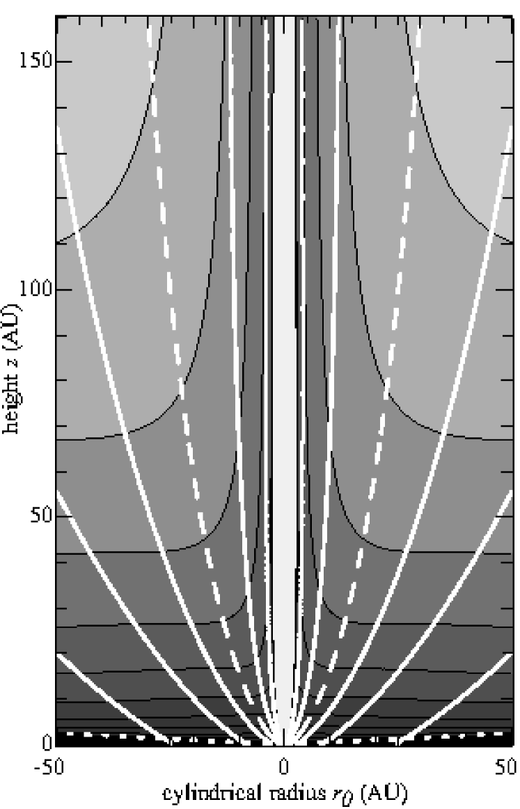
Figure 1: Overall geometry of the ”slow” MHD disk wind solution of (Casse & Ferreira, 2000) used in this article. Solid white curves show various magnetic flow surfaces, with that anchored at 1 AU shown in dashed. The density for $\dot{M}_{\mathrm{acc}}=10^{-6}M_{\odot}/{\rm yr}$ and $M_{\star}=0.5M_{\odot}$, is coded in the contour plot starting at $8\times 10^{4}\leavevmode\nobreak\ \mathrm{cm}^{-3}$ and increasing by factors of 2. The bottom dotted line traces the slow magnetosonic surface (at 1.7 disk scale heights) where our chemical integration starts. A color version of this figure is available in the online edition of this journal.

”Slow” MHD solutions ($\lambda<20$) that become super Alfvénic may be obtained by including a small entropy deposition at the disk upper layers $z\simeq h$ (Casse & Ferreira, 2000). The warm mass-loading region is denser and the ejection efficiency $\xi$ is substantially enhanced, lowering the $\lambda$ value (see eq. 1). Such additional heating was assumed to be powered by dissipation of MHD disk turbulence and parametrized as a tiny fraction $f$ of the disk accretion power, with $f=8\times 10^{-4}$ in the solution chosen here (see Casse & Ferreira 2000 for a discussion of the effect of $f$ on the wind dynamics). This new class of solutions, referred to as ”warm” in Pesenti et al. (2004), is still ”cold” in a dynamical sense as the initial thermal energy remains negligible compared to gravity, and the wind acceleration is still mostly magnetic. Therefore, the wind temperature beyond the slow point does not affect the dynamics and we may recompute it a posteriori from the actual heating/cooling terms, without loss of self-consistency (see discussions in Section 4 and Appendix A).

Other input properties of the adopted solution are: a thermal (uncompressed) aspect ratio $\varepsilon=h/r=C_{s}/V_{K}=0.03$ (with $C_{s}$ the sound speed and $V_{K}$ the kepler speed), a turbulent resistivity in the disk midplane $\nu_{\rm m}=\alpha_{\rm m}V_{\rm A,0}h$, with $V_{\rm A,0}$ the Alfvén velocity and $\alpha_{\rm m}=2$ (in order to ensure stationarity), and a turbulent viscosity $\nu_{v}=\nu_{m}$. Crossing of the slow magnetosonic point is obtained for a ratio of magnetic to thermal pressure in the disk midplane $\mu\simeq 0.33$ (leading to quasi-keplerian rotation; Shu et al. 2008). The computed second Blandford & Payne jet parameter is $\kappa\simeq 0.1$, and the field inclination at the disc surface is $\theta_{0}\simeq 57.3^{\circ}$, with similar surface values of $B_{z}$, $B_{\phi}$ and $B_{r}$.

For a given self-similar MHD solution, all physical quantities at a given polar angle obey specific scalings with the stellar mass $M_{\star}$, the disk accretion rate $\dot{M}_{\mathrm{acc}}$, and the anchoring radius $r_{0}$ of the magnetic surface in the midplane, as given in eq. (9) of Garcia et al. (2001a). In particular, the midplane field in the adopted MHD solution is,

$$B_{z}\simeq 0.7G\left(\frac{r_{0}}{1\,{\rm AU}}\right)^{-5/4}\left(\frac{\dot{M}_{\mathrm{acc}}}{10^{-6}M_{\odot}{\rm yr}^{-1}}\right)^{1/2}\left(\frac{M_{\star}}{0.5M_{\odot}}\right)^{1/4},$$ (3)

which follows the same scaling as the available magnetic field measurements in protostellar disks (Shu et al., 2007). The required field strengths thus appear plausible. In the following, we will vary $M_{\star}$, $\dot{M}_{\mathrm{acc}}$, and $r_{0}$ in order to explore their effect on the molecular content and thermal state of the disk wind.

2.2 Thermo-chemical evolution

The thermo-chemical evolution along wind streamlines was implemented by adapting the last version (Flower & Pineau des Forêts, 2003) of a code constructed to calculate the steady-state structure of planar molecular MHD multi-fluid shocks in interstellar clouds (Flower et al., 1985). The ion-neutral drift, FUV field, and dust-attenuation were calculated following the methods developed by Garcia et al. (2001a) in the atomic disk wind case. Irradiation by stellar X-rays was also added, following the approach of Shang et al. (2002).

Given the high densities and low ion-neutral drift speeds in the wind (see Section 3) the same temperature and velocity is adopted here for all particles. The latter is prescribed by the underlying single-fluid MHD wind solution. We thus integrate numerically the following differential equations on mass density $\rho$, species number density $n(a)$, and temperature $T$ along the streamline, as a function of altitude $z$ above the disk midplane:

$$\frac{\mathrm{d}\rho_{f}}{\mathrm{d}z} = \frac{S_{f}-\rho_{f}\nabla\cdot\mathbf{v}}{v_{z}},$$ (4)

$$\frac{\mathrm{d}n(a)}{\mathrm{d}z} = \frac{R_{a}-n(a)\nabla\cdot\mathbf{v}}{v_{z}},$$ (5)

$$\frac{\mathrm{d}T}{\mathrm{d}z} = \frac{\Gamma-\Lambda-n_{\rm tot}k_{B}T\nabla\cdot\mathbf{v}-\frac{3}{2}k_{B}TR}{\frac{3}{2}k_{B}n_{\rm tot}v_{z}}.$$ (6)

Here, $v_{z}$ and ($\nabla\cdot\mathbf{v}$) are the bulk vertical flow speed and the (3D) flow divergence interpolated from the MHD wind solution, $n_{\rm tot}$ is the total number density of particles, $T$ is the temperature, $k_{B}$ is the Boltzmann constant, $S$ and $R$ are the rates of change in mass and number of particles, respectively, per unit volume, and $\Gamma$ and $\Lambda$ are the heating and cooling rates per unit volume. The equations on $n(a)$ apply to each species $a$ as well as to the individual populations of the first 49 levels of H₂ (up to an energy of $20\,000$ K) which are integrated in parallel with the other variables. The equations on $\rho_{f}$ apply to each ”fluid” $f$ (neutral, positive, negative) and are used mainly for internal checking purposes, as the total mass density $\rho(z)$ is prescribed by the MHD solution.

Cooling and heating mechanisms include

• Radiative cooling by H₂ lines excited by collisions with H, H₂, He, and electrons (Le Bourlot et al., 1999).

• Radiative cooling by CO, H₂O, and ¹³CO in the Large Velocity Gradient approximation (Neufeld & Kaufman, 1993), and by OH and NH₃ in the low-density limit (Flower et al., 1985).

• Atomic cooling by fine-structure and metastable lines of C, N, O, S, Si, C⁺, N⁺, O⁺, S⁺, Si⁺ (Flower et al., 2003) and Fe⁺ (Giannini et al., 2004).

• Inelastic scattering of electrons on H and H₂ (Aggarwal et al., 1991; Hummer, 1963; Rapp & Englander-Golden, 1965).

• Energy released by collisional ionisation and dissociation and exo/endo-thermicity of chemical reactions (Flower et al., 1985).

• Energy heat/loss through thermalization with grains (Tielens & Hollenbach, 1985).

• Ambipolar-diffusion heating by elastic scattering between the neutral fluid and charged ions and grains (Garcia et al. 2001a, see Section 2.3).

• Ohmic heating arising from the drift between electrons and other fluids (Garcia et al. 2001a, see Section 2.3).

• Photoelectric effect on grains (Bakes & Tielens, 1994, eq. 42) irradiated by the (attenuated) FUV field of hot accretion spots (see Section 2.4).

• Heating through cosmic-rays and (attenuated) coronal stellar X-rays (Dalgarno et al. 1999; see Section 2.5).

The reader is referred to the corresponding references for a discussion of the physical context and hypotheses involved in modelling each of the above processes.

2.2.1 Chemical network

The chemical network consists of 134 species, including atoms and molecules (either neutral or singly ionized) as well as their correspondents inside grain refractory cores, and on grain icy mantles. A representative polycyclic aromatic hydrocarbon (PAH) with 54 carbon atoms is also included, with a fractional abundance of $10^{-6}$ per H nucleus. The total elemental abundances and their initial distribution among gas, grain cores, and icy mantles are taken from Tables 1 and 4 of Flower & Pineau des Forêts (2003).

The charge balance of grains and PAHs is treated as in Flower & Pineau des Forêts (2003). The number of grains per H nucleus and the mean grain cross section are determined from the abundance of depleted elements in grain cores, and the adopted grain size distribution (see Section 2.4.2). Most of the grains are charged, and assumed well-coupled to the charged fluid.

We consider 1143 reactions including neutral-neutral and ion-neutral reactions, recombination with electrons, charge exchange, cosmic ray induced desorption from grains, sputtering of grain icy mantles, and erosion of charged grain cores by impact of drifting heavy neutral species. Reaction rates between charged and neutral species are enhanced by ion-neutral drift, following the effective temperature prescription of Flower et al. (1985), with the drift speed $\mathbf{v}_{in}$ computed as described in Section 2.3.

H₂ collisional dissociation is treated level by level following Le Bourlot et al. (2002). Reformation on grains is computed with the sticking coefficient of Hollenbach & McKee (1979). Three-body reactions in the gas phase are not included, therefore we will limit ourselves to densities $\leq 10^{12}$ cm^-3.

Ionisation and dissociation reactions by far-ultraviolet (FUV) photons from accretion hot spots, and by stellar coronal X-rays, are included as described in Sections 2.4 and 2.5, respectively.

2.2.2 Initial conditions and integration

The integration of the set of equations for temperature, mass and number of particles along the flow is an initial value problem. Thus initialization of temperature and initial populations have to be devised. As in Garcia et al. (2001a), we start all calculations from the wind slow magnetosonic point (located at $1.66h(r)$ for our adopted MHD solution), and assume that the temperature and species abundances there are at equilibrium with the local radiation field. These equilibrium values are obtained by performing a ”steady-state” run over $10^{5}$ yrs where thermo-chemical equations are solved with the density held fixed. We then integrate the thermo-chemical equations along the flow using the DVODE integrator (Brown et al., 1989), until the recollimation point where the streamline reaches its maximum radial extension (radius of $40r_{0}$ at $z=900r_{0}$ for our chosen wind solution). We checked that the final temperature and H₂ abundance along the streamline do not depend sensitively on the initial equilibrium conditions, as long as the gas is fully molecular initially. This occurs because the ionisation (which controls the ion-neutral drift heating) adjusts rapidly at the dense wind base to the local radiation field, even though it becomes frozen-in at large distances.

2.3 Ambipolar diffusion coefficients

The ambipolar diffusion and Ohmic heating terms require a detailed calculation of elastic momentum exchange rates and drift speeds. The ion-neutral drift speed is calculated from the MHD solution using the analytical formula derived in Appendix A of Garcia et al. (2001a), valid for $||\mathbf{v}_{in}||\ll||\mathbf{v}||$:

$$\mathbf{v}_{in} = \frac{1}{1+p}\left(\frac{\mathbf{J}\times\mathbf{B}}{c(1+X)\overline{\mu_{in}n_{i}\nu_{in}}}+p\frac{\mathbf{J}}{q_{e}n_{e}}\right)$$ (7)

$$p = \frac{\overline{\mu_{en}n_{e}\nu_{en}}}{\overline{\mu_{in}n_{i}\nu_{in}}}$$ (8)

where $\mathbf{J}$ is the electric current density, $\mathbf{B}$ is the magnetic field, $c$ is the speed of light, $q_{e}$ is the electron charge, $n_{e}$ and $n_{i}$ are the number densities of electrons and ions, $X=\rho_{i}/\rho_{n}$, and $\overline{\mu_{in}n_{i}\nu_{in}}$ and $\overline{\mu_{en}n_{e}\nu_{en}}$ are the total momentum transfer rate coefficients for ion-neutral and electron-neutral collisions, respectively.

The total ion-neutral momentum transfer rate coefficient is obtained by summing over the main neutrals (H, H₂, He) and over all ions, charged PAHs and charged grains:

$$\overline{\mu_{in}n_{i}\nu_{in}}=\sum_{\begin{array}[]{c}a=\mathrm{ions},\\ \mathrm{PAH}^{\pm},g^{\pm}\end{array}}\sum_{\begin{array}[]{c}b=\\ \mathrm{H},\mathrm{H}_{2},\mathrm{He}\end{array}}\mu_{ab}n(a)n(b)\left<\sigma v\right>_{ab},$$ (9)

where $n(a)$ is the number density of species $a$, $\mu_{ab}$ is the reduced mass of particles $a$ and $b$, and $\left<\sigma v\right>_{ab}$ is their elastic collision rate coefficient; the latter is evaluated via the recent analytical fits to quantum-mechanical calculations provided in Table 2 of Pinto & Galli (2008a), when available, given as a function of the effective relative speed $\bar{v}$:

$$\bar{v} = \sqrt{\frac{8k_{B}T_{r}}{\pi\mu_{ab}}+||\mathbf{v}_{in}||^{2}}$$ (10)

$${\rm with}\quad T_{r} = \frac{m_{a}T_{n}+m_{b}T_{i}}{m_{a}+m_{b}}.$$ (11)

For the H₂-H⁺ pair we use the updated fit in Pinto & Galli (2008b). For the rest of the pairs $\left<\sigma v\right>_{ab}$ is taken as the maximum of the polarizability and hard sphere rate coefficients (Garcia et al., 2001a):

$$\left<\sigma v\right>_{ab}=\max\left\{2.41\pi q_{e}\sqrt{\frac{\alpha_{b}}{\mu_{ab}}},\sigma_{s}\bar{v}\right\},$$ (12)

where $\alpha_{b}$ is the polarizability of H, He, or H₂ and the hard sphere cross section is taken as

$$\sigma_{s}=\left\{\begin{array}[]{lll}10^{-14}\leavevmode\nobreak\ \mathrm{cm}^{2}&,&\mathrm{PAH}^{\pm}\\ \pi\left<R_{d}^{2}\right>&,&\mathrm{grains}\ (g^{\pm})\\ 10^{-15}\leavevmode\nobreak\ \mathrm{cm}^{2}&,&\mathrm{else}\end{array}\right.$$ (13)

Here $\pi\left<R_{d}^{2}\right>$ denotes the average grain cross section over our size distribution. The total momentum transfer rate coefficient for collisions between electrons and neutrals is given by:

$$\overline{\mu_{en}n_{e}\nu_{en}}=m_{e}n_{e}\sum_{a=\mathrm{H},\mathrm{H}_{2},\mathrm{He}}n(a)\left<\sigma v\right>_{ea}$$ (14)

with the $\left<\sigma v\right>_{ea}$ also evaluated from the recent analytical fits of Pinto & Galli (2008a). The ion-electron momentum transfer rate entering Ohmic heating is calculated with the classical formula of Schunk (1975) (see eq. A.13 of Garcia et al. 2001a).

Fig. 2 plots the momentum transfer rate coefficients (normalized by $n_{\mathrm{H}}^{2}$) for collisions between the neutral fluid and the different charged fluids as a function of vertical distance above the disk midplane for a representative streamline. It may be seen that collisions with positive ions dominate the coupling, with an extra contribution from charged PAHs near the flow base.

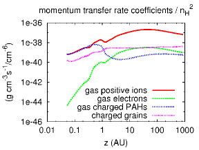
Figure 2: Momentum transfer rate coefficients (normalized by $n_{\mathrm{H}}^{2}$) in collisions of the neutral fluid with the different charged fluids as a function of altitude along a flow line launched at 1 AU, for $\dot{M}_{\mathrm{acc}}=10^{-6}M_{\odot}$ yr^-1, $M_{\star}=0.5M_{\odot}$ (our Class I model). A color version of this figure is available in the online edition of this journal.

The ambipolar drag heating and Ohmic heating are given by (Garcia et al., 2001a):

$$\Gamma_{\mathrm{drag}}=\left(\frac{{\rho_{n}}}{\rho}\right)^{2}\frac{\frac{1}{c^{2}}\|\@vec{J}\times\@vec{B}\|^{2}}{\overline{\mu_{in}n_{i}\nu_{in}}},\quad\Gamma_{\mathrm{ohm}}={\eta}\|\@vec{J}\|^{2},$$ (15)

with $\eta=(\overline{\mu_{ie}n_{i}\nu_{ie}}+\overline{\mu_{en}n_{n}\nu_{ne}})/(q_{e}n_{e})^{2}$. Note that $\Gamma_{\mathrm{drag}}$ is proportional to the square of the Lorentz force per particle, and inversely proportional to the ionisation fraction in the wind.

2.4 FUV field

The FUV radiation will control the ion abundance (and therefore the ion-neutral drift) in the upper wind regions. It will also photodissociate molecules, and provide extra heating by collisions with warm dust and photoelectric effect on grains. Our treatment essentially follows the approach of Garcia et al. (2001a) with several updates, including an accretion spot geometry and a photochemical network.

2.4.1 Unattenuated radiation field

Instead of the optically thick equatorial boundary layer model adopted in Safier (1993) and Garcia et al. (2001a), we adopt here the paradigm of magnetospheric accretion, recently favored in T Tauri stars, where the inner disk is truncated at several stellar radii and accreting material flows along field lines in quasi free-fall, giving rise to shocked ”hot spots” on the stellar surface (Bouvier et al., 2007). The accretion geometry in younger protostars is not yet constrained observationally, but their similar X-ray flare properties to T Tauri stars indicate an already well-developed stellar magnetosphere (Imanishi et al., 2003), hence we will adopt the same paradigm for simplicity.

The FUV radiation field thus comes from the central low-mass star of effective temperature $T_{\star}=4\,000$ K, and from hot accretion spots of fixed temperature $T_{\mathrm{hs}}=10\,000$ K, chosen to match the mean observed colour temperature of the FUV excess in T Tauri stars (Johns-Krull et al., 2000). Both radiation sources are treated as black bodies.

As in Garcia et al. (2001a), we neglect the scattering contribution to the FUV field. The (unattenuated) direct stellar flux at distance $R$ from the star (with dimensions erg cm^-2 s^-1 Hz^-1) is calculated through the relation

$$F_{\nu}(R)=\left(B_{\nu}(T_{\star})+B_{\nu}(T_{\mathrm{hs}})\delta_{\mathrm{hs}}\right)\frac{\pi R_{\star}^{2}}{R^{2}}$$ (16)

where $B_{\nu}(T)$ denotes the specific intensity at frequency $\nu$ of a black body of temperature $T$, $R_{\star}$ is the stellar radius, and $\delta_{\mathrm{hs}}$ is the fraction of the total stellar surface $4\pi R_{\star}^{2}$ covered by hot spots (assumed uniformly distributed). The main difference with the boundary-layer model of Garcia et al. (2001a) is thus a fixed $T_{\mathrm{hs}}$ independent of $\dot{M}_{\mathrm{acc}}$, and a more isotropic radiation flux (due to the lack of projection effects or disk occultation).

In each model, $\delta_{\mathrm{hs}}$ is determined by requiring that the hot spots radiate half of the accretion luminosity, i.e. $4\pi R_{\star}^{2}\delta_{\mathrm{hs}}\sigma_{B}T_{\mathrm{hs}}^{4}=G\dot{M}_{\mathrm{acc}}M_{\star}/(2R_{\star})$. The value of one half is meant to be illustrative only: the actual fraction of accretion luminosity radiated in the accretion shock could exceed 80% for a large disk truncation radius $>5R_{\star}$, or decrease if a sizeable fraction of accretion energy is tapped to drive a stellar wind. None of these effects being well quantified, especially in Class 0 and Class I sources, we adopt 50% here for illustration and consistency with the boundary-layer model of Garcia et al. (2001a). We set $R_{\star}=3R_{\odot}$, the radius of a young accreting $0.5M_{\odot}$ star near the ”birthline” with $T_{\star}=4\,000$ K according to the models of Stahler (1988), noting that it remains a good approximation for a very young Class 0 ($R_{\star}\simeq 2R_{\odot}$ for a $0.1M_{\odot}$ protostar accreting at $5\times 10^{-6}M_{\odot}\mathrm{yr}^{-1}$; cf. Stahler 1988). With the above assumptions, the modelled FUV hot spot continuum in the domain $1\,400-2\,000$ Å is a factor $1.5-2.5$ stronger than the accretion shock models of Gullbring et al. (2000) for DR Tau and DG Tau, using the same accretion rates ($\dot{M}_{\mathrm{acc}}=3-5\times 10^{-7}M_{\odot}$ yr^-1). On the other hand, if the FUV spectrum below $1\,400$ Å were as flat as in the lower accretion stars BP Tau and TW Hya (Bergin et al., 2003), our blackbody model would underestimate the flux at $1\,000$ Å by a factor $4-2$. This remains sufficiently accurate for the present exploratory study.

Since we do not solve for radiative transfer, we neglect the extra FUV flux in the stellar Ly$\alpha$ line. Ly$\alpha$ pumping of highly excited levels of H₂ is occuring close to the star (Herczeg et al., 2002, 2006; Nomura & Millar, 2005) but will be less important on the larger jet scales of interest here, especially since we focus on dense molecular jets where H₂ is well shielded.

2.4.2 Attenuation by dust

The stellar FUV field is attenuated mainly by dust in the disk wind along the line of sight to the star. The sublimation radius $R_{\mathrm{sub}}$ is calculated via eq. (B.5) of Garcia et al. (2001a), considering a unique sublimation temperature $T_{\rm sub}=1\,500$ K. We used the dust optical properties tabulated by Draine & Lee (1984); Draine & Malhotra (1993); Laor & Draine (1993), assuming the standard ”MRN” mixture of astronomical silicates and graphite and the grain radius distribution $n(a)\propto a^{-3.5}$ proposed by Mathis et al. (1977), with grain radii in the interval [0.005,0.25] $\mu$m. The sublimation surface for the Class 0/I/II models in Section 3 is plotted in Fig. 3 on top of inner disk wind streamlines.

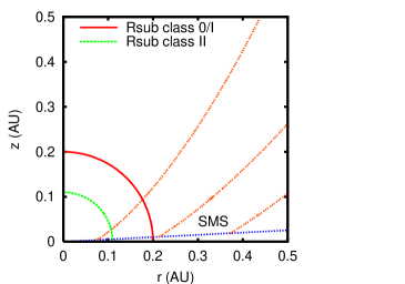
Figure 3: The dust sublimation surface in our Class 0/I models (outer red circle) and our Class II model (inner green circle), for the grain size distribution and mixture of silicates and graphite proposed by Mathis et al. (1977). The wind slow magnetosonic surface (denoted SMS) is superimposed as well as three flow lines (orange dotted lines), including the innermost one launched from 0.07 AU. The stellar parameters are $T_{\star}=4\,000$ K and $R_{\star}=3R_{\odot}$, while the hot spot temperature and coverage fraction are $T_{\mathrm{hs}}=10\,000$ K, and $\delta_{\mathrm{hs}}=0.032$ (Class 0/I) and 0.0032 (Class II). A color version of this figure is available in the on-line edition of this journal.

The dust optical depth to the star at point of spherical coordinates $(R,\theta)$ is $\tau_{\nu}(R,\theta)=\overline{\sigma_{d}(\nu)}N_{\mathrm{H}}^{d}(R,\theta)$ where $\overline{\sigma_{d}(\nu)}$ is the dust extinction cross section per H nucleus (integrated over the grain size distribution), and $N_{\mathrm{H}}^{d}(R,\theta)$ is the column density of hydrogen nuclei on dusty wind streamlines along the line of sight to the star. In our self-similar wind model, the wind density varies as $R^{-1.5}f(\theta)$, and $N_{\mathrm{H}}^{d}(R,\theta)$ may then be integrated analytically as:

$$N_{\mathrm{H}}^{d}(R,\theta)=2n_{\mathrm{H}}(R,\theta)R\left(\sqrt{\frac{R}{R_{\rm min}(\theta)}}-1\right).$$ (17)

Here, $n_{\mathrm{H}}$ is the number density of H nuclei in all forms, $n_{\mathrm{H}}\simeq n(\mathrm{H})+2n(\mathrm{H}_{2})+n(\mathrm{H}^{+})$, and $R_{\rm min}(\theta)$ is the spherical radius inside which there is no dust, i.e. either the sublimation radius, $R_{\mathrm{sub}}$, or the radius of the innermost flow line at angle $\theta$, $R_{\rm in}(\theta)$, whichever is larger (see Fig. 3). The innermost wind streamline is assumed launched from $r_{\rm in}=0.07$ AU, a typical corotation radius in young low-mass stars.

The total dust geometrical cross section per H nucleus, calculated from our grain size distribution and the abundance of depleted elements in grain cores, is $\pi\left<R_{d}^{2}\right>n_{d}/n_{\mathrm{H}}=1.36\times 10^{-21}\leavevmode\nobreak\ \mathrm{cm}^{2}$, where $\left<R_{d}^{2}\right>$ is the mean square grain radius; the ratio of $A_{V}$ to $N_{\mathrm{H}}$ is then $\overline{\sigma_{d}(5500\leavevmode\nobreak\ \AA)}=2.72\times 10^{-22}\leavevmode\nobreak\ \mathrm{cm}^{2}$.

2.4.3 Dust temperature

Collisions with dust grains heated by the UV field can be an important gas heating/cooling term at the wind base (though unimportant further out). We assume that above the wind slow point ($z\geq 1.7h$), dust is optically thin to its own radiation. The dust temperature is then calculated at every step from the grain radiation equilibrium against incident (wind-attenuated) stellar photons:

$$4\pi\sigma_{B}T_{d}^{4}\left<R_{d}^{2}\right>\cdot\overline{\left<Q_{\mathrm{em}}(T_{d})\right>}=\int_{0}^{\infty}\overline{\sigma_{d}(\nu)}F_{\nu}(R)\mathrm{e}^{-\overline{\sigma_{d}(\nu)}N_{\mathrm{H}}^{d}(R,\theta)}\mathrm{d}\nu$$ (18)

where $\sigma_{B}$ is the Stefan-Boltzmann constant, $\left<R_{d}^{2}\right>$ is the mean square grain radius, $\overline{\left<Q_{\mathrm{em}}(T_{d})\right>}$ is the Planck-averaged grain emission efficiency (weighted by $n(a)a^{2}$), and $\overline{\sigma_{d}(\nu)}$ is the dust absorption cross section per H nucleus defined earlier. Collisions with the gas are neglected in the grain thermal balance, as they compete with radiation only at densities $>10^{13}\leavevmode\nobreak\ \mathrm{cm}^{-3}$ (Glassgold et al., 2004). We verified that when the FUV excess and the wind attenuation are negligible, our $T_{d}$ values agree with detailed calculations at the top of the disk atmosphere by D’Alessio et al. (1999) for MRN dust and a $4\,000$ K star (taking into account differences in $R_{\star}$).

2.4.4 Photochemical network

A network of photoionisation and photodissociation reactions is implemented with rates in the form $k_{p}=\chi\,\gamma\mathsf{e}^{-\beta A_{V}}$, where $A_{V}$ is the visual extinction calculated above (Section 2.4.2), $\beta,\gamma$ are constants depending on the reaction, taken from van Dishoeck (1988) and Roberge et al. (1991), and $\chi$ is the ratio at $1\,000$ Å of the unattenuated FUV flux to the mean interstellar radiation field of Draine (1978), integrated over $4\pi(\mathrm{2\times 10^{-6}\,erg\leavevmode\nobreak\ s^{-1}\leavevmode\nobreak\ cm^{-2}}$ Å${}^{-1})$. Such a ”monochromatic” flux normalization at $1\,000$ Å was chosen rather than the average ratio to the interstellar field over the interval $910-2\,066$ Å, denoted $G_{0}$ in the literature (see e.g. Tielens & Hollenbach 1985), as photoreactions contributing to the main ionisation and dissociation reactions in our models (C, S, CH⁺, H₂, CO) occur in the narrow range $910-1\,200$ Å.

Special cases of photodissociation reactions are the dissociation of H₂ and CO, which occur through line absorption. We thus need to consider not only the shielding caused by the dust particles, but also the additional self and cross shielding due to those species themselves. They were implemented in the model in an approximate way as described below.

2.4.5 H₂ photodissociation.

We adopted an H₂ photodissociation rate coefficient per molecule of the form proposed by Draine & Bertoldi (1996):

$$k_{p,\mathrm{H}_{2}}=\chi\,p_{0}({\mathrm{H}_{2}})\,\times f_{\mathrm{H}_{2},d}(A_{V})f_{\mathrm{H}_{2},\mathrm{H}_{2}}(N_{\mathrm{H}_{2}},b)$$ (19)

where $p_{0}({\mathrm{H}_{2}})=4.2\times 10^{-11}$ s^-1 is the unshielded rate in the Draine field, $f_{\mathrm{H}_{2},d}(A_{V})=\mathrm{e}^{-\beta_{d}A_{V}}$ is the shielding factor by dust, with $\beta_{d}=\sigma_{d}({1000\leavevmode\nobreak\ \AA})/\sigma_{d}({5500\leavevmode\nobreak\ \AA})=6.3$ for our dust mixture, and $f_{\mathrm{H}_{2},\mathrm{H}_{2}}(N_{\mathrm{H}_{2}},b)$ is the H₂ self-shielding factor given by eq. (37) in Draine & Bertoldi (1996), with the line width parameter $b$ set here to the local sound speed $C_{s}$. The shielding column of H₂ molecules on the line of sight to the star, $N_{\mathrm{H}_{2}}$, depends on the H₂ abundance on all inner wind streamlines. In order to allow a local calculation in the present exploratory study, we assume a mean H₂ abundance on the line of sight to the star equal to half the local H₂ abundance at the current point of the streamline. This ”local” assumption tends to overestimate self-shielding, but will not affect our results when photodissociation is not the dominant destruction mechanism. A conservative check of this hypothesis is made a posteriori (see Section 3).

2.4.6 CO photodissociation.

For CO, one needs to consider not only the self-shielding and the shielding by dust, but also the shielding by H₂ (through line overlap with CO). We have fitted the data of Table 11 from Lee et al. (1996) as a function of $A_{V}$ and of the shielding columns $N_{\mathrm{CO}}$ and $N_{\mathrm{H_{2}}}$, and obtained the following analytical formulae for the shielding factors by dust, CO, and H₂ respectively:

$$f_{\mathrm{CO,d}}(A_{V}) = \max\left\{0.5\mathrm{e}^{-3.5A_{V}},0.1\mathrm{e}^{-3A_{V}}\right\},$$ (20)

$$f_{\mathrm{CO,CO}}(N_{\mathrm{CO}}) = \min\left\{1,\left(\frac{N_{\mathrm{CO}}}{10^{15}\leavevmode\nobreak\ \mathrm{cm}^{-2}}\right)^{-0.75}\right\},$$ (21)

$$f_{\mathrm{CO,H_{2}}}(N_{\mathrm{H_{2}}}) = 0.8\mathrm{e}^{-N_{\mathrm{H}_{2}}/1.7\times 10^{21}\leavevmode\nobreak\ \mathrm{cm}^{-2}}.$$ (22)

These analytical formulas are valid to within a factor of 2 up to $N_{\mathrm{CO}}\simeq 2\times 10^{19}\leavevmode\nobreak\ \mathrm{cm}^{-3}$, and over the whole range in $N_{\mathrm{H}_{2}}$ and $A_{V}$, as shown in Figure 4.

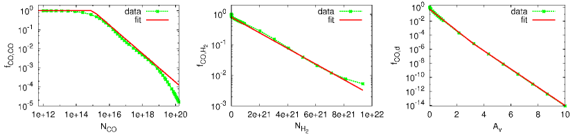
Figure 4: Adopted analytical fits (red curves, from eq. 22) to the CO photodissociation shielding factors of Lee et al. (1996) (connected green symbols) caused by CO line overlap (left), H₂ line overlap (middle) and dust extinction (right).

The photodissociation rate coefficient per molecule is then

$$k_{p,{\rm CO}}=\chi p_{0}({\rm CO})\times f_{\mathrm{CO},d}(A_{V})f_{\mathrm{CO,CO}}(N_{\mathrm{CO}})f_{\mathrm{CO},\mathrm{H}_{2}}(N_{\mathrm{H}_{2}}),$$ (23)

where $p_{0}({\rm CO})=2\times 10^{-10}$s^-1 is the unshielded rate for an isotropic Draine field (twice the value from Lee et al. (1996), who assume a one-sided cloud illumination). As done for H₂, the shielding column of CO molecules on the line of sight to the star, $N_{\mathrm{CO}}$, is calculated assuming a mean CO abundance on inner disk streamlines of half the local value of the CO abundance at the current point.

2.5 X-rays

Hard coronal X-rays will be the dominant ionization process at the base of the dusty disk wind, where the stellar FUV flux is strongly extinguished by dense inner streamlines. Energetic secondary electrons generated by X-ray ionisation will also dissociate and heat the gas. Our adopted X-ray treatment and chemical network are described in the following.

2.5.1 X-ray spectrum and attenuation

The X-ray flux is modelled as a thermal spectrum with characteristic energy $kT_{X}$,

$$F_{X}(E)\equiv\mathrm{d}L_{X}(E)/dE=(L_{X}/kT_{X})\times\exp(-E/kT_{X})$$

The attenuated rate of X-ray energy deposition per H nucleus in the wind writes

$$H_{X}(R,\theta)=\int^{\infty}_{E_{0}}\frac{F_{X}(E)}{4\pi R^{2}}\sigma_{\mathrm{pe}}(E)\exp^{-\sigma_{\mathrm{pe}}(E)N_{\mathrm{H}}(R,\theta)}\mathrm{d}E,$$ (24)

where $E_{0}$ is the low energy cutoff of the incoming X-ray spectrum, $\sigma_{\mathrm{pe}}(E)$ is the photoelectric cross section per H nucleus, and $N_{\mathrm{H}}(R,\theta)$ is the total column of H nuclei to the star through inner wind streamlines (given by eq. 17 with $R_{\rm min}(\theta)=R_{\rm in}(\theta)$). We calculate $H_{X}$ analytically following Glassgold et al. (1997) and Shang et al. (2002), who adopted a low-energy cutoff $E_{0}=0.1$ keV and a power-law approximation to the cross section, $\sigma_{\mathrm{pe}}(E)=2.27\times 10^{-22}\leavevmode\nobreak\ \mathrm{cm}^{-2}\leavevmode\nobreak\ (\mathrm{KeV}/E)^{p}$ with $p=2.485$. $H_{X}$ then writes

$${H_{X}}(R,\theta)=H_{0}(R)I_{p}(\xi_{0},\tau_{X})$$ (25)

where

$$H_{0}(R) = \frac{L_{X}}{4\pi R^{2}}{\sigma_{\mathrm{pe}}(kT_{X})},$$ (26)

$$I_{p}(\xi_{0},\tau_{X}) = \int_{\xi_{0}}^{\infty}\mathrm{e}^{-(\xi+\tau_{X}\xi^{-p})}\xi^{-p}\mathrm{d}\xi\simeq J_{p}(\tau_{X}),$$ (27)

$\xi_{0}=E_{0}/kT_{X}$, $\tau_{X}\equiv\sigma_{\mathrm{pe}}(kT_{X})N_{\mathrm{H}}(R,\theta)$ is the X-ray optical depth at $kT_{X}$, and $J_{p}(\tau_{X})$ is an analytical fit given in eq. (C3) of Shang et al. 2002, and plotted in Fig. 5. The fit is valid for $\tau_{X}>\tau_{0}=1/p\xi_{0}^{p}(p+\xi_{0})=10^{-4}$, a condition verified in our models.

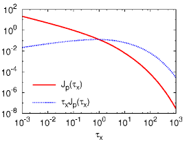
Figure 5: The function $J_{p}(\tau_{X})$ describing the attenuation of the energy deposition rate by a thermal X-ray spectrum versus $\tau_{X}$, the X-ray optical depth at the characteristic energy, $kT_{X}$. Also plotted is the function $\tau_{X}J_{p}(\tau_{X})$ describing the effect of changing $kT_{X}$ (i.e. $\tau_{X}$) for a fixed attenuating gas column density (see eq. 28).

The effect of changing $kT_{X}$ for a fixed $L_{X}$ and fixed position $(R,\theta)$ (and therefore a fixed attenuating column $N_{\mathrm{H}}$) may be visualised by rewriting $H_{X}$ as

$${H_{X}}(R,\theta)=H_{0}(R)J_{p}(\tau_{X})=\tau_{X}J_{p}(\tau_{X})\times L_{X}/(4\pi R^{2}N_{\mathrm{H}}).$$ (28)

The function $\tau_{X}J_{p}(\tau_{X})$, also plotted in Fig. 5, is almost flat over a broad range of $\tau_{X}$ (0.001 to 100). The regions where X-ray ionisation dominates in our models have values of $\tau_{X}\simeq 0.3-30$ within this range for $kT_{X}=4$ keV. Furthermore, the ionization fraction varies only with the square root of ${H_{X}}$. Varying $kT_{X}$ in the range $2.5-15$ keV (i.e. $\tau_{X}$ in the range $0.01-100$) would thus not strongly modify our results.

2.5.2 X-ray ionization rates

X-ray ionization rates are calculated with the same simplifying assumptions as in Glassgold et al. (1997) and Shang et al. (2002): The mean energy to form an $A^{+}$ ion is approximated by its constant high-energy limit $W(A^{+})$, valid for primary photoelectrons with $E>E_{0}=0.1$ keV. Neglecting the small difference in energy between the absorbed X-ray photon and the primary photoelectron, and recalling that the absorbed energy $H_{X}$ is per H nucleus, the X-ray ionization rate of species $A$ per atom is then given by

$$\zeta(A^{+})=\frac{H_{X}n_{\mathrm{H}}}{W(A^{+})}\frac{1}{n(A)}$$ (29)

The limiting mean energies $W(A^{+})$ for X-ray ionization of H₂, H, and He in neutral gas mixtures with 10% of Helium have been calculated by Dalgarno et al. (1999) who fitted them as linear functions of $n(\mathrm{H})/n(\mathrm{H}_{2})$ (middle terms of eq. 30-32 below). We further simplify their expressions by taking $0.53\simeq 0.5$, $1.89\simeq 2$, and recalling that the number density of H nuclei $n_{\rm H}\simeq n(\mathrm{H})+2n(\mathrm{H}_{2})$ at low ionization, and $n(\mathrm{He})=0.1n_{H}$, which yields the right-hand side terms:

$$W(\mathrm{H}_{2}^{+}) = 41.9{\rm eV}\left[1+0.53\frac{n(\mathrm{H})}{n(\mathrm{H}_{2})}\right]\simeq 20{\rm eV}\frac{n_{\mathrm{H}}}{n(\mathrm{H}_{2})},$$ (30)

$$W(\mathrm{H}^{+}) = 39.5{\rm eV}\left[1+1.89\frac{n(\mathrm{H}_{2})}{n(\mathrm{H})}\right]\simeq 40{\rm eV}\frac{n_{\mathrm{H}}}{n(\mathrm{H})},$$ (31)

$$W(\mathrm{He}^{+}) = 470{\rm eV}\simeq 47.0{\rm eV}\frac{n_{\mathrm{H}}}{n(\mathrm{He})}.$$ (32)

Inserting the right-hand side expressions for $W(A^{+})$ in eq. (29), the X-ray ionization rates per specie $A$ become independent of $n_{\rm H}$ and $n(A)$ and may be written solely in terms of the parameter $\zeta(\mathrm{H}_{2}^{+})$ that enters our chemical network:

$$\zeta(\mathrm{H}_{2}^{+}) \equiv H_{X}/20{\rm eV},$$ (33)

$$\zeta(\mathrm{H}^{+}) \simeq 0.5\zeta(\mathrm{H}_{2}^{+}),$$ (34)

$$\zeta(\mathrm{He}^{+}) \simeq 0.4\zeta(\mathrm{H}_{2}^{+}).$$ (35)

The total ionization rate per H nucleus, often denoted $\zeta_{X}$ in the literature, is related to $\zeta(\mathrm{H}_{2}^{+})$ by

$$\zeta_{X} = \zeta(\mathrm{H}_{2}^{+})\frac{0.5n(\mathrm{H})+n(\mathrm{H}_{2})+0.4n(\mathrm{He})}{n_{H}}$$ (36)

$$= 0.54\zeta(\mathrm{H}_{2}^{+}),$$ (37)

regardless of the ratio H/H₂. The formation of H⁺ through dissociative ionization of H₂ is also included with a rate of $\zeta(\mathrm{H}_{2}^{+})/22$ per molecule (Dalgarno et al., 1999). A constant cosmic ray ionization rate $\zeta_{\rm CR}(\mathrm{H}_{2}^{+})=5\times 10^{-17}$ s^-1 is added to the rate produced by stellar X-rays, but it plays a negligible role in our models.

2.5.3 X-ray induced dissociation

The rate of H₂ dissociation by X-ray induced electrons is taken as $0.5\zeta(\mathrm{H}_{2}^{+})$, following the results of Dalgarno et al. (1999) for primary electron energies $>0.1$ keV. The energetic electrons also collisionally excite H₂ to higher electronic levels, which then radiatively decay by emitting a flux of ultraviolet ”secondary photons” able to dissociate other molecular species. We adopt the dissociation factors $p_{M}$ calculated by Gredel et al. (1989) for various species, leading to a rate per unit volume of $\zeta(\mathrm{H}_{2}^{+})[n(\mathrm{H}_{2})/n_{\mathrm{H}}]n(M)p_{M}/(1-\omega)$ (Flower et al., 2007), where we adopt a grain albedo $\omega=0.5$. For CO, we adopt the high-abundance, high-temperature limit of $p_{\rm CO}=28$ for $\omega=0.5$ (Gredel et al., 1987). Photodetachment of electrons from PAHs by secondary photons is also included (Flower & Pineau des Forêts, 2003).

2.5.4 X-ray heating

The heating efficiency of the X-rays and cosmic rays is treated collectively. We use the results of Dalgarno et al. (1999), who studied the heating produced by high energy electrons interacting with a partly ionized gas mixture of H, H₂ and 10% of He. The heating efficiency $\eta_{h}$ is calculated for ionization fractions $<0.1$ and includes the fraction of initial primary electron energy lost by elastic scattering with neutrals and electrons and by rotational excitation of H₂ (rapidly thermalized at our densities). The total heating rate per unit volume by X-rays and cosmic rays is given by:

$$\Gamma_{\mathrm{X+CR}}(z)=\eta_{h}H_{X}n_{\mathrm{H}}=\frac{10r\eta_{\mathrm{H}_{2}}+\eta_{\mathrm{H}}}{10r+1}\zeta(\mathrm{H}_{2}^{+})\epsilon_{\mathrm{H}_{2}}n_{\mathrm{H}}$$ (38)

where $\epsilon_{\mathrm{H}_{2}}=20$ eV follows from the definition of $\zeta(\mathrm{H}_{2}^{+})$ in eq. (33), $r=n(\mathrm{H}_{2})/n(\mathrm{H})$, and $\eta_{\mathrm{H}_{2}},\eta_{\mathrm{H}}$ are respectively the heating efficiencies for the H₂-He and the H-He ionized mixtures, fitted as a function of the electron fraction $x_{\rm e}=n_{\rm e}/n_{\mathrm{H}}$ in the form

$$\eta=1+\frac{\eta_{0}-1}{1+cx_{\rm e}^{a}}$$ (39)

with $\eta_{0}=0.055$, $c=2.170$, $a=0.366$ for H₂-He, and $\eta_{0}=0.117$, $c=7.950$, $a=0.678$ for H-He (Dalgarno et al., 1999, Table 7).

3 Results

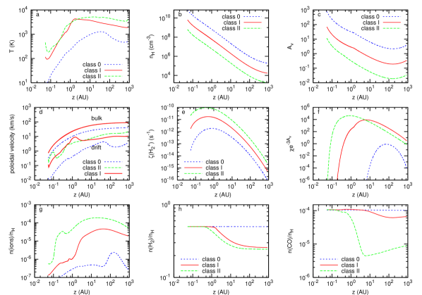
Figure 6: Various variables along a flow line anchored at 1 AU, for the dense MHD disk wind solution and three typical classes of stars: class 0 ($M_{\star}=0.1M_{\odot}$, $\dot{M}_{\mathrm{acc}}=5\times 10^{-6}M_{\odot}$ yr^-1; dotted blue curves), class I ($M_{\star}=0.5M_{\odot}$, $\dot{M}_{\mathrm{acc}}=10^{-6}M_{\odot}$ yr^-1; solid red curves) and active class II ($M_{\star}=0.5M_{\odot}$, $\dot{M}_{\mathrm{acc}}=10^{-7}M_{\odot}$ yr^-1; dashed green curves). (a) The gas temperature $T$; (b) the number density of hydrogen nuclei $n_{\mathrm{H}}$; (c) the visual extinction $A_{V}$ to the star, in magnitudes; (d) the poloidal components of the bulk flow speed $v$ (smooth top curves) and calculated drift speed $v_{in}$ (lower 3 curves); Note that the Class II and Class I have the same $M_{\star}$, hence the same bulk flow speed for $r_{0}=1$ AU; (e) the X-ray H₂ ionization rate per molecule $\zeta(\mathrm{H}_{2}^{+})$; (f) the effective radiation field in Draine units $\chi\exp^{-3A_{V}}$ (attenuation factor appropriate for carbon photoionisation); (g) the fractional abundance of ions; (h) the fractional abundance of $\mathrm{H}_{2}$ (upper limit in the Class II model, see Section 3.1.3); (i) the fractional abundance of CO (upper limits in the Class I/II models, see Section 3.1.4). A color version of this figure is available in the on-line edition of this journal.

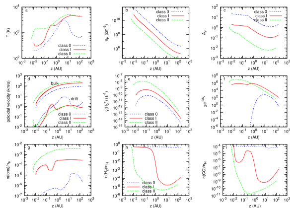
Figure 7: Same as Figure 6 for streamlines anchored just beyond the sublimation radius: $r_{0}=R_{\mathrm{sub}}=0.2$ AU in the Class 0 and Class I, and 0.11 AU in the Class II. These calculations assume no self-shielding of H₂ or CO (i.e. no molecules surviving on streamlines launched inside $R_{\mathrm{sub}}$). The resulting abundances set a minimum photodissociation timescale on outer streamlines, to be compared with the flow timescale (see Figure 10). A color version of this figure is available in the on-line edition of this journal.

To investigate how the chemical content of protostellar disk winds evolves in time with the decline of accretion rate, we considered three sets of parameters representative of the main evolutionary stages of young low-mass stars with bright jets:

• a very young Class 0 protostar ($\dot{M}_{\mathrm{acc}}=5\times 10^{-6}M_{\odot}$ yr^-1, $M_{\star}=0.1M_{\odot}$), where accretion is high and the star has not yet reached its final mass; the chosen parameter values describe e.g. the heavily embedded sub-millimeter exciting source of the HH 212 jet (Lee et al., 2006).

• a Class I source ($\dot{M}_{\mathrm{acc}}=10^{-6}M_{\odot}$ yr^-1, $M_{\star}=0.5M_{\odot}$), where the star has accumulated most of its final mass, but residual infall and accretion still proceed at a fast pace; the chosen parameters describe e.g. the infrared exciting source of HH26 (Antoniucci et al., 2008).

• an active Class II star ($\dot{M}_{\mathrm{acc}}=10^{-7}M_{\odot}$ yr^-1, $M_{\star}=0.5M_{\odot}$), representative of optically visible T Tauri stars with bright optical microjets, e.g. DG Tau or RW Aur (Gullbring et al., 2000).

With our choice of parameters, and the self-similar scalings of the MHD solution, the wind density $n_{H}\propto\dot{M}_{\mathrm{acc}}M_{\star}^{-1/2}r_{0}^{-1.5}$ drops by a factor 10 from one Class to the next. Our adopted stellar radius of $3R_{\odot}$ gives the same accretion luminosity of $5L_{\odot}$ in the Class 0 and Class I models, and 10 times smaller in the Class II, leading to a hot spot coverage fraction $\delta_{\mathrm{hs}}$ of 3.2% and 0.32% respectively (cf. Section 2.4.1).

We adopt a thermal X-ray spectrum of characteristic energy $kT_{X}=4$ keV and luminosity $L_{X}=10^{30}$ erg/s, typical of the ”hard” time-variable component in solar-mass young stars and jet-driving protostars (Imanishi et al., 2003; Güdel et al., 2007). $L_{X}$ is a time-averaged value of 30% of the median flare luminosity in solar-mass YSOs, based on a typical flare interval of 4-6 days (Wolk et al., 2005). The exact value of $kT_{X}$ has no major effect on our results (see Section 2.5.1).

Note that the flow crossing timescale out to the recollimation point is very short, only 50 yrs for a streamline launched at 1 AU in the Class I model. The chemical composition of the disk wind will thus deviate substantially from published ”static” disk atmosphere models such as, e.g. Glassgold et al. (2004); Nomura & Millar (2005). The presence of adiabatic cooling and drag heating also introduce major differences in the thermal structure. These effects are discussed in Section 4.

We first analyse in detail the results obtained for the 3 evolutionary classes, for a representative anchor radius $r_{0}=1$ AU, and for a streamline launched just outside sublimation, $r_{0}\simeq R_{\mathrm{sub}}$. The effect of increasing $r_{0}$ is discussed later on, in Section 3.2.

3.1 Results for $r_{0}=1$ AU and $r_{0}=R_{\mathrm{sub}}$ for the 3 classes

Figure 6 shows the main physical parameters integrated as a function of $z$ along the 1 AU streamline for the Class 0/I/II models: temperature, ion-neutral drift speed, ionisation fraction, H₂ and CO abundance. Also plotted are the (prescribed) flow density and bulk speed, and the calculated $A_{V}$ to the central star, attenuated X-ray ionisation rate of H₂, and ”effective” FUV field at $1\,000$ Å in Draine units (e${}^{-3A_{V}}$ being the attenuation factor for Carbon photoionisation in our chemical network). In Figure 7, we show for comparison the results obtained for streamlines with an anchor radius just beyond the sublimation radius, computed assuming no H₂ or CO self-shielding (i.e. assuming no molecules on streamlines launched inside $R_{\mathrm{sub}}$).

3.1.1 Radiation field and ionization structure

The ionization fraction is a key parameter governing the temperature profile, through the drag heating term. It is controlled by attenuation of the radiation field through inner wind streamlines. The behavior is qualitatively similar along the streamlines launched from 1 AU and from $R_{\mathrm{sub}}$.

The A_V towards the star is highest at the wind base, where the line of sight crosses the densest wind layers (see Fig. 1) and drops steadily as material climbs along the streamline (Figure 6-7c). This causes a steep rise in the effective attenuated radiation field, until the $1/R^{2}$ dilution factor takes over (Fig. 6-7e,f). Combined with the wind density fall-off (Fig. 6-7b), this generates a global increase in ionisation fraction along the streamlines out to $30-100$ AU, until recombination sets in (Fig. 6-7g). In our models, ionization is dominated by stellar X-rays for $A_{V}>3$ mag, and by FUV photons further out.

As the wind density drops by a factor 10 from Class 0 to Class I to Class II (Fig. 6-7b), the ionisation fraction, $X({\rm i}^{+})\equiv n({\rm ions})/n_{\mathrm{H}}$, increases by a factor 3 to 10. Indeed, the smaller attenuating column through the inner wind (Fig. 6-7c) leads to higher X-ray and FUV ionization rates. At the same time, the lower wind density reduces recombination. Both effects work in the same direction.

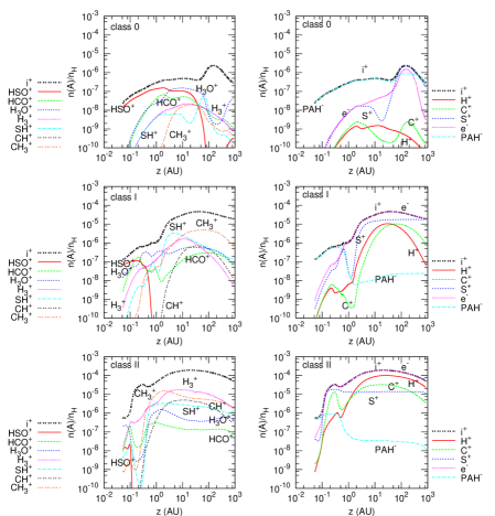
Figure 8: The main ionization contributors along a disk wind streamline launched from 1 AU, for our Class 0, Class I, and Class II models (top to bottom). The left panels plot the fractional abundances relative to H nuclei of molecular ions; the right-hand panels plot abundances of atomic ions and negative species (electrons and PAH^-). The total ionisation fraction, $X({\rm i}^{+})\equiv n({\rm ions})/n_{\mathrm{H}}$, is also plotted as a thick black curve. A color version of this figure is available in the on-line edition of this journal.

Figure 9: The main cooling (left panels) and heating (right panels) processes along a disk wind streamline launched from 1 AU, for our Class 0, Class I, and Class II models (top to bottom). The heat transfer from grain to gas, $\Gamma_{g,n}$, appears in the cooling curves when negative, and in the heating curves when positive. Other plotted cooling/heating terms are: $\Lambda_{\rm adia}$: adiabatic cooling; $\Lambda_{\rm H_{2},H_{2}O,CO}$: line cooling from H₂, H₂O, CO; $\Gamma_{\rm drag}$: ambipolar diffusion heating; $\Gamma_{\rm ohm}$: ohmic heating; $\Gamma_{\rm g,photo}$: photoelectric effect on grains; $\Gamma_{\rm X,cr}$: X-ray and cosmic ray heating. OH line cooling never dominates and is not plotted for clarity. A color version of this figure is available in the on-line edition of this journal.

Fig. 8 shows the main ionization contributors along the 1 AU streamline for the Class 0, Class I, and Class II models. From these results, it can be seen that the main contributors depend on the overall ionization degree, $X({\rm i}^{+})$:

when $X({\rm i}^{+})\leq 10^{-6}$:

The main contributors to the negative charge are the PAHs. The main positive carriers are molecular ions, with the most abundant being HSO⁺ and H₃O⁺; and H${}_{3}^{+}$ (a direct product of X-ray ionization) also contributing in the Class II.

when $X({\rm i}^{+})>10^{-6}$:

The main contributors to the negative charge are the electrons. The main positive carriers are the atomic ions S⁺, C⁺, and H⁺, which recombine more slowly with electrons than molecular ions do.

An interesting result of our calculations is the relatively high abundances of CH⁺, SH⁺, and H⁺ of $10^{-6}-10^{-4}$ reached along the Class I and Class II streamlines (Fig. 8). CH⁺ and SH⁺ are formed by endothermic reaction of C⁺ and S⁺ with H₂, when the wind temperature exceeds about $3\,000$ K. H⁺ forms by X-ray ionisation and charge exchange, but also by photodissociation of CH⁺, with carbon playing the role of a catalyst through the reaction chain:

$$\mathrm{C}+{h\nu} \rightarrow \mathrm{C}^{+},$$ (40)

$$\mathrm{C}^{+}+\mathrm{H}_{2} \rightarrow \mathrm{C}\mathrm{H}^{+}+\mathrm{H}-4640\ \mathrm{K},$$ (41)

$$\mathrm{C}\mathrm{H}^{+}+{h\nu} \rightarrow \mathrm{C}+\mathrm{H}^{+}.$$ (42)

Through this repeated formation cycle, H₂ is partly converted into H⁺, helping to offset H⁺ destruction by charge exchange. The flow crossing timescale is also too short for significant H⁺ radiative recombination. This example clearly illustrates the out-of-equilibrium and hybrid nature of the chemistry in MHD disk winds, combining elements from both C-shocks (strong heating by ion-neutral drift) and photo-dissociation regions (abundant C⁺ and S⁺).

3.1.2 Drift speed, heating/cooling processes, and temperature behavior

Thanks to X-ray and UV ionization, we find that the drift speed remains relatively low along the streamlines, at 10% of the bulk poloidal speed or less, as seen in Fig. 6-7d. This validates a posteriori the single fluid approximation made in computing the MHD dynamical solution. It also keeps the drag heating and gas temperature to a moderate value. Note that the ratio of drift speed to poloidal speed scales as $v_{in}/V_{\rm p}\propto M_{\star}\dot{M}_{\mathrm{acc}}^{-1}X({\rm i}^{+})^{-1}<\sigma v>_{in}^{-1}$, so that the single fluid approximation remains fulfilled in the Class 0 jet (small $M_{\star}$, large $\dot{M}_{\mathrm{acc}}$) despite its low ionisation.

The main heating and cooling terms for $r_{0}=1$ AU are plotted in Fig. 9. Collisions with warm dust can be important near the wind base when densities exceed a few $10^{9}$ cm^-3, but ambipolar ”drag” heating by ion-neutral collisions, $\Gamma_{\rm drag}$, quickly prevails as density drops. The predominance of ambipolar diffusion over other sources of heating (shocks excepted) is a widespread characteristic of steady MHD-driven protostellar winds from low-mass sources, and results from the strong accelerating $\mathbf{J}\times\mathbf{B}$ force combined with a low wind ionisation (see Ruden et al., 1990; Safier, 1993; Garcia et al., 2001a). Cooling is dominated by adiabatic expansion out to $z\simeq 1$ AU, and by radiative cooling further out, due to the high molecular abundances. The main coolant is H₂ in the Class I and Class II models, and H₂O in the Class 0 model.

The resulting behavior of temperature along the 1 AU streamlines is qualitatively similar regardless of the accretion rate (Fig. 6a): After initial cooling due to adiabatic expansion, drag heating takes over and heats up the gas to $1\,000-5\,000$ K. This leads to a sharp increase in molecular cooling (denoted $\Lambda_{\rm rad}$ thereafter) which (assisted by collisional dissociation cooling in the Class I/II models) eventually overcomes $\Gamma_{\rm drag}$, leading to a temperature turnover followed by a slow decline where both terms remain in close balance.

The balance between $\Gamma_{\rm drag}$ and $\Lambda_{\rm rad}$ on the 1 AU wind streamline is maintained thanks to the powerful thermostatic behavior of molecular cooling, which is highly sensitive to temperature. Any slight excess/deficit of drag heating leads to an increase/decrease in radiative cooling until the two terms match again. In the outer wind, radiative cooling approaches the low-density limit (i.e. $\Lambda_{\rm rad}\simeq n_{\mathrm{H}}^{2}f_{\rm rad}(T)$), therefore the asymptotic jet temperature profile is determined by the condition $f_{\rm rad}(T)\simeq\Gamma_{\rm drag}/n_{\mathrm{H}}^{2}$. The latter term slowly declines with distance in our models, leading to the slowly declining temperature. Furthermore, the self-similar scalings for $\@vec{J},\@vec{B},n_{\mathrm{H}}$ in eq. (9) of Garcia et al. (2001a) yield a scaling for $\Gamma_{\rm drag}/n_{\mathrm{H}}^{2}\propto M_{\star}^{3}\dot{M}_{\mathrm{acc}}^{-2}r_{0}^{-1}X({\rm i}^{+})^{-1}$, explaining why we find much cooler jets in the Class 0 case. Final temperatures are only $\sim 500-700$ K, compared to $2\,000$ K in the Class I, and $3\,000$ K in the Class II models.

The streamlines from $r_{0}=R_{\mathrm{sub}}$ in the Class I and II cases show a slightly different asymptotic temperature behavior, with a flatter isothermal ”plateau” at large distances (Fig. 7a). Molecules are heavily photodissociated on these two streamlines, so that ambipolar diffusion heating is balanced by adiabatic cooling alone. The flat temperature ”plateau” resulting from this balance between $\Gamma_{\rm drag}$ and $\Lambda_{\rm adia}$ is a well known typical property of atomic self-similar MHD disk winds (Safier, 1993; Garcia et al., 2001a). The lower atomic plateau temperature $\simeq 4\,000$ K found here, compared to $\simeq 10^{4}$ K in Garcia et al. (2001a), results from our different adopted MHD wind solution, which is typically 2 times slower and 5 times denser (see Section 2.1).

It is also noteworthy that, for both values of $r_{0}$, the initial temperature rise is much slower in the Class 0 jet; as shown in Garcia et al. (2001a) (equations 24 and 26), the slope of the initial temperature rise, where $\Lambda_{\rm adia}$ dominates the cooling, is determined by the ratio of $\Gamma_{\rm drag}$ to $\Lambda_{\rm adia}$, which scales as $M_{\star}^{2}/(\dot{M}_{\mathrm{acc}}r_{0})$ in self-similar disk winds for a fixed ionisation fraction. This scaling is smaller in our Class 0 than in our Class I case by a factor $5^{3}=125$, explaining the delay to heat the gas in the Class 0 jet despite a 10 times lower ionisation fraction than in the Class I jet.

3.1.3 H₂ survival

The calculated H₂ abundances along streamlines launched from 1 AU and from $R_{\mathrm{sub}}$ are plotted in Fig. 6-7h, for the 3 classes of sources. Below, we first analyse the results in detail for the Class I case, and then discuss the Class II and Class 0 cases.

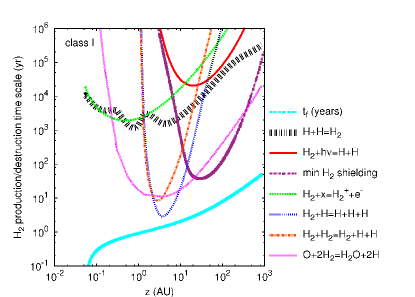
Figure 10: The net timescales (after subtraction of any reverse reaction rate) of the principle reactions that form or destruct H₂ are plotted versus altitude along a streamline launched at 1 AU for our Class I model. The flow crossing timescale $t_{\rm f}$ is also plotted at the bottom for comparison. Thin curves denote reactions whose net effect leads to destruction, and thick curves those that lead to net creation. The reactions are $\mathrm{H+H=H_{2}}$: catalytic formation of H₂ on grains; $\mathrm{H_{2}+h\nu=H+H}$: photodissociation (with the minimum self-shielded rate shown on a separate curve); $\mathrm{H_{2}+x=H_{2}^{+}+e^{-}}$: X-ray ionisation; $\mathrm{O+2H_{2}=H_{2}O+2H}$: combined oxydation reactions with O and OH; $\mathrm{H_{2}+H}$ and $\mathrm{H_{2}+H_{2}}$: collisional dissociation. The latter becomes very efficient near $z\simeq 2$ AU, where the wind temperature reaches $4\,000$ K. A color version of this figure is available in the on-line edition of this journal.

Class I case:

The streamline launched just outside $R_{\mathrm{sub}}=0.2$ AU suffers heavy H₂ destruction (see Fig. 7h). Self-shielding is not operative (we assumed no molecules on inner, dust-free streamlines) and the FUV field is very strong. Hence most H₂ molecules are quickly photodissociated at $z\simeq 1$ AU. Balance with reformation on dust yields a final H₂ abundance $\simeq 10^{-4}$.

In contrast, half of the H₂ molecules are found to survive along the 1 AU streamline (see Fig. 6h). This may be understood by examining the timescales of the main formation/destruction processes of H₂ along this streamline, plotted in Fig. 10. The flow timescale up to the current point, $t_{\rm f}$, is also plotted for comparison and is seen to be very short (50 yrs out to $1\,000$ AU). With our assumption of a mean H₂ abundance of half the local value, the self-shielded H₂ photodissociation timescale (red curve in Fig. 10) is now much longer than the flow timescale. As a conservative check of this conclusion, we also plot in Fig. 10 (thick pink curve with symbols) the minimum H₂ photodissociation timescale, where $N(\mathrm{H}_{2})$ and the corresponding self-shielding factor are calculated assuming an H₂ abundance on inner streamlines equal to its minimum value, as obtained on the streamline $r_{0}=R_{\mathrm{sub}}$. Even in this overly pessimistic case, the minimum H₂ photodissociation timescale remains an order of magnitude longer than the flow time at all $z$ (Fig. 10), confirming that H₂ will escape photodissociation on the 1 AU streamline in the Class I model.

Only two processes are found to be fast enough to affect the H₂ abundance on the 1 AU streamline: The first to occur is endothermic neutral-neutral reactions with O and OH to form H₂O and H atoms (denoted collectively as $\mathrm{O+2H_{2}=H_{2}O+2H}$ in Fig. 10):

$$\mathrm{O}+\mathrm{H}_{2} \rightarrow \mathrm{O}\mathrm{H}+\mathrm{H}-2980\ \mathrm{K}$$ (43)

$$\mathrm{O}\mathrm{H}+\mathrm{H}_{2} \rightarrow \mathrm{H}_{2}\mathrm{O}+\mathrm{H}-1490\ \mathrm{K}.$$ (44)

The second process is collisional dissociation by H and H₂. The timescale shortens by 6 orders of magnitude as temperature increases from $2\,000$ K to $4\,000$ K, and approaches the flow time around $z\simeq 2$ AU, so that half of H₂ is destroyed by 10 AU. Further out, collisional dissociation shuts off due to both the temperature decline and the density fall-off; the H₂ abundance thus remains ”frozen-in” at half its initial value (Fig. 6h). We conclude that streamlines will turn from mostly atomic to mostly molecular around $r_{0}\simeq 1$ AU for our Class I model.

Active Class II case:

The H₂ abundance shows a similar behavior to the Class I case. The streamline from $R_{\mathrm{sub}}$ suffers heavy photodissociation, with a final abundance of $\simeq 2\times 10^{-5}$ (Fig. 7h), while half of the molecules survive on the 1 AU streamline (Fig. 6h). However, the minimum photodissociation timescale on the 1 AU streamline, computed with the same method as above, is now shorter than the flow time around $z\simeq 30$ AU; therefore, our local approximation to self-shielding might significantly underestimate H₂ photodestruction on the Class II streamline launched at 1 AU. Our H₂ abundance in this particular case should thus be viewed conservatively as an upper limit, pending more detailed non-local calculations.

Class 0 case:

Here, wind densities are so high that dust screening against photodissociation is very effective, even on the streamline just outside $R_{\mathrm{sub}}$. In addition, temperature is so low that oxydation reactions and collisional dissociation are slower than the flow crossing time, except briefly on the $R_{\mathrm{sub}}$ streamline. Therefore, the Class 0 disk wind retains $90\%-100\%$ of its full initial H₂ content on dusty streamlines launched from $r_{0}\geq R_{\mathrm{sub}}=0.2$ AU.

3.1.4 Main O, C, and S-bearing species along the 1 AU streamline

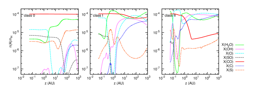
Figure 11: Abundances relative to H nuclei of important O, C, and S-bearing species along a flow line launched at 1 AU, for our Class 0 (left), Class I (middle) and Class II models (right). A color version of this figure is available in the on-line edition of this journal.

The fractional abundances of the main O- and C-bearing neutral species with respect to H nuclei are plotted in Fig. 11 along the 1 AU streamline for the 3 classes of sources. S and SO are also plotted, as they were identified recently as tracers of molecular jets in Class 0 sources (Dionatos et al., 2009, 2010; Tafalla et al., 2010).

CO:

We find that no CO destruction occurs on the Class 0 streamline from 1 AU, thanks to the very efficient dust shielding provided by dense inner wind layers. In contrast, CO is partly destroyed by FUV photodissociation along the Class I/II streamlines. Once the FUV field drops down, CO reforms mainly through the reaction $\mathrm{HCO^{+}+e^{-}}\rightarrow\mathrm{CO+H}$ but the timescale is longer than the flow time and the final abundance per H nucleus is only $5\times 10^{-5}$ in the Class I jet, and $10^{-5}$ in the Class II jet. These latter values should be considered conservatively as upper limits, as CO self-shielding could be significantly overestimated by our approximate ”local” treatment (see Section 3.2 below). We thus predict an abundance ratio of H₂/CO $\geq 0.5\times 10^{4}$ in all cases.

H₂O:

When the wind temperature exceeds $\simeq 400$ K, oxygen not locked in CO is converted to H₂O through the endothermic reactions of O and OH with H₂ in eq. (43)-(44). Together with H₃O⁺ recombination, this reaction is efficient enough to balance the water destruction processes active in Class I/II jets (FUV photodissociation, photoionisation, reaction with H${}_{3}^{+}$). The asymptotic abundance of water is thus similar and quite high on the 1 AU streamline for all 3 classes, at $\simeq 5-10\times 10^{-5}$.

C, O, S atoms, OH and SO:

OH and atomic C and O have low abundances along the Class 0 streamline, where CO and H₂O are well shielded. In contrast, high abundances of these species $\simeq 0.5-1\times 10^{-4}$ are predicted in the outer regions of the Class I and Class II streamlines, following CO and H₂O partial photodissociation (see Fig. 11). Concerning sulfur, it is mainly in the form of atomic S beyond 100 AU along the Class 0 streamline, and is mainly photoionized into S⁺ in the Class I/II cases, where the FUV field is more intense (see Fig. 8). The asymptotic abundance of SO is substantial in the Class 0 only, at a level of $3\times 10^{-7}$. These predicted characteristics for Class 0 jets are in line with the relative abundance of SO to CO $\simeq 2\times 10^{-3}$ reported by Tafalla et al. (2010), and with the mass-flux traced by atomic sulfur lines being possibly as large as that inferred from CO (Dionatos et al., 2010).

3.2 Effect of increasing launch radius in the Class I model

In Fig. 12 we illustrate in the Class I case the effect of the launch radius on the wind chemistry and temperature. We plot a range of $r_{0}$ of $1-9$ AU corresponding to a range in final flow speed of $90\leavevmode\nobreak\ \mathrm{km\leavevmode\nobreak\ s}^{-1}$ to $30\leavevmode\nobreak\ \mathrm{km\leavevmode\nobreak\ s}^{-1}$. The streamline from $R_{\mathrm{sub}}=0.2$ AU is also shown for comparison. The main effect is that the flow has an ”onion-like” thermal-chemical structure, with streamlines launched from larger radii having higher H₂ abundance and lower temperature and ionization. The behavior with $r_{0}$ is discussed in more detail below.

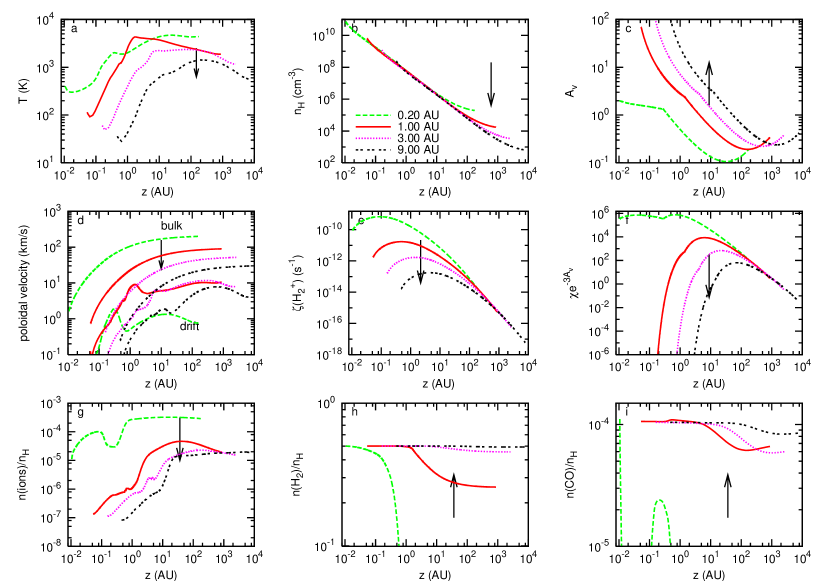
Figure 12: Thermo-chemical structure for a range of streamlines in our Class I jet: $R_{\mathrm{sub}}\simeq 0.2$ AU(green dashed, taken from Fig. 7), Class I jet: 0.34 AU (blue dotted), 0.58 AU (green solid), 1 AU (red solid), 3 AU (pink dotted), and 9 AU (black dashed). The arrow shows the effect of increasing launch radius on the plotted quantities, which are the same as in Fig. 6. CO abundances are upper limits, except on the $r_{0}=R_{\mathrm{sub}}$ streamline (calculated with no self-shielding). A color version of this figure is available in the on-line edition of this journal.

We do not present results for the interval $0.2<r_{0}<1$ AU in the Class I jet, as the minimum H₂ photodissociation timescale there becomes similar to or less than the flow time (see discussion in Section 3.1.3). Accurate H₂ abundances on these inner streamlines await a detailed non-local treatment of H₂ shielding, not taken into account in the present preliminary approach. For the same reason, we do not present results at $r_{0}>1$ AU for the Class II jet, but we note that the effect of increasing $r_{0}$ will be qualitatively the same as in the Class I case (i.e. higher H₂ abundance and lower temperature). We also do not present results at $r_{0}>1$ AU in the Class 0 case, since most H₂ and CO molecules survive already at a launch radius just beyond the sublimation radius $R_{\mathrm{sub}}=0.2$ AU (see Section 3.1.3).

3.2.1 Ionisation and drift speed at various $r_{0}$

Wind streamlines are initially less ionised at larger $r_{0}$ (Fig. 12f,g), due to the larger attenuation of X-rays and FUV photons by intervening streamlines (Fig. 12c). At large distances, they recombine to an asymptotic fractional ionisation of a few $10^{-5}$, dominated by S⁺.

The drift speed does not exceed about $10\leavevmode\nobreak\ \mathrm{km\leavevmode\nobreak\ s}^{-1}$ and remains less than 30% of the bulk flow speed out to $r_{0}=9$ AU (Fig. 12d). Therefore, magnetocentrifugal forces appear able to lift molecules out to disk radii of 9 AU for the typical parameters of Class I sources, in the MHD solution investigated here.

3.2.2 Temperature and molecule survival at various $r_{0}$

The gas temperature at larger launch radii follows a similar behavior to that found at $r_{0}=1$ AU (i.e. a gradual rise on a scale $z\simeq r_{0}$, followed by a shallow decrease), but the temperature peak is shifted to larger $z$ (i.e. lower $n_{\mathrm{H}}$) and reaches a smaller peak value (see Fig. 12a). Therefore, H₂ chemical oxydation and collisional dissociation are less efficient than for $r_{0}=1$ AU. As a result, the H₂ abundance increases with $r_{0}$ and more than 90% of the molecules survive for launch radii $\geq 3$ AU (Fig. 12h). Photodissociation of H₂, which was already too slow for $r_{0}=1$ AU, is further reduced by the additional screening from intervening wind streamlines and plays no role.

In contrast, we find that photodissociation remains the major destruction process for CO out to $r_{0}=9$ AU. The drop in CO abundance towards the inner $r_{0}=R_{\mathrm{sub}}$ streamline largely exceeds the factor 2 assumed in our ”local” computation of the CO self-screening column (see Fig. 12i). The plotted CO abundances for $r_{0}>R_{\mathrm{sub}}$ should thus be considered as upper limits only, and a detailed non-local treatment of self-shielding will be needed to obtain more accurate values.

4 Discussion

4.1 Comparison with static disk atmosphere models

It is instructive to compare our results with thermo-chemical calculations of irradiated static molecular disks at a radius of 1 AU. Glassgold et al. (2004) focussed on X-ray disk irradiation, with a similar X-ray flux to ours ($L_{X}=2\times 10^{30}$ erg s^-1, $kT_{X}=1$ keV). Nomura & Millar (2005) studied FUV irradiation by the star with standard ISM dust properties as adopted here, and a mean unshielded flux at a distance of 140 AU of $G_{0}\simeq 1\,000$ times the mean interstellar flux, averaged over the interval $910-2\,000$ Å (see their Fig. 4), similar to our Class I case (see Fig. 6f).

We find that the thermo-chemical structure of MHD disk winds launched from 1 AU in Class I sources markedly differs from irradiated static disks at the same radius: H₂ survives to much greater altitudes and the gas temperature rises more gradually. We briefly discuss and explain these differences below.

4.1.1 H₂ survival and wind shielding

In static disk models at 1 AU, H₂ is destroyed by X-rays or FUV photons above $z\simeq 0.1$ AU (Glassgold et al., 2004; Nomura & Millar, 2005). In contrast, on the 1 AU streamline of the Class I disk wind, half of the gas remains molecular beyond $z\simeq 10$ AU and until the end of the streamline (Fig. 6h). The survival of H₂ against photodissociation arises from several effects:

1. The first key effect is the enhanced screening provided by dense inner wind streamlines compared to a hydrostatic flared disk geometry. As shown in Fig. 1, the self-similar MHD disk wind solution chosen here produces density contours that are horizontal just above the disk surface. In contrast, density contours in a hydrostatic disk are strongly flared out, allowing a more direct illumination of the disk surface by the central star (see Fig. 1 of Nomura & Millar 2005). This difference is illustrated by the large $A_{V}$ values towards the central star in Fig. 6c; in the Class I streamline at 1 AU, the ”effective” dust-attenuated FUV field at $z\simeq 0.3$ AU is $\chi\exp^{-3A_{V}}\simeq 2$ compared to $G_{0}\simeq 10^{7}$ in the static disk of Nomura & Millar (2005) at the same $(r,z)$. The peak X-ray ionisation rate is $\zeta(\mathrm{H}_{2}^{+})\simeq 2\times 10^{-11}$ s^-1, instead of $6\times 10^{-9}$ s^-1 at the top of the disk atmosphere in Glassgold et al. (2004).

2. The second key factor is the very short flow timescale; only 50 years from the slow point out to $1\,000$ AU for the 1 AU streamline. Static disk models assume chemical equilibrium, so that H₂ disappears wherever destruction reactions are faster than reformation. In disk winds, H₂ can still survive this situation as long as the destruction time is longer than the flow time (see Fig. 10).

4.1.2 Gas temperature profile

In static disk models at 1 AU, FUV photoelectric heating or X-ray heating induce a sharp increase in gas temperature up to $1\,500-5\,000$ K within a few scale heights, at $z/r_{0}\simeq 0.15-0.2$ (Nomura & Millar, 2005; Glassgold et al., 2004). In our disk wind model, the rise in temperature is much more gradual, with temperatures of a few thousand K reached only around $z/r_{0}\simeq 1$. This difference stems both from the greater attenuation of X-rays and FUV photons by inner wind streamlines, and from the powerful adiabatic expansion cooling experienced by the wind after launching. The latter term largely exceeds FUV and X-ray heating and is only slightly offset by drag heating (see Fig. 9), yielding a slow net heating rate. A related consequence is that temperatures above $2\,000$ K are reached only in wind regions of low density so that H₂ collisional dissociation and chemical oxydation is limited.

4.2 Limitations of the model and planned improvements

The results presented here are only a preliminary attempt at addressing the highly complex problem of the coupled ionisation, chemical, thermal, and dynamical structure of MHD disk winds from young stars. Several limitations have been introduced that we discuss below with our planned improvements:

1. We ignored feed-back of the thermal structure on the dynamics. This is in fact well justified because thermal pressure gradients are already negligible above the slow point where our integration starts, and are only dynamically important in the mass-loading region located deeper in the disk, around $z\simeq h$ (see Casse & Ferreira 2000). Therefore, any deviations between our computed wind temperature and the prescription adopted by Casse & Ferreira (2000) to compute the dynamical solution do not alter the self-consistency of the model. Nevertheless, we show in Appendix A that the two temperatures fall close to each other near the wind base. The existence of such ”slow” warm MHD solutions might then be a natural outcome of the heating mechanisms present near the surface of an irradiated molecular disk. Thermal calculations extending into the optically thick and resistive mass-loading region are under way to test this conjecture (Garcia et al., in preparation).

2. We also ignored feed-back of the ion-neutral drift on the flow dynamics; we showed that this single fluid approximation is well fulfilled at launch radii $\leq 9$ AU but tends to degrade at larger $r_{0}$ or small $\dot{M}_{\mathrm{acc}}$, due to the scaling of $v_{\rm in}/V_{\rm p}\propto X({\rm i}^{+})^{-1}\dot{M}_{\mathrm{acc}}^{-1}$. Therefore, ion-neutral drift may be one of the factors (together with the available magnetic flux) limiting the outer radial extension of molecular MHD disk winds in young stars. The drift will also decrease rotation signatures in neutral jet tracers at large $r_{0}$ compared to the single fluid prediction. Multi-fluid MHD calculations would be useful to further quantify this effect.

3. We adopted a simplified treatment of shielding against photodissociation. An upcoming improvement of our model will be the inclusion of a non-local treatment of the self-screening, in order to obtain more accurate predictions of CO and/or H₂ abundances in the Class I and Class II jets.

   Shielding against photodissociation also depends on the assumed composition of inner wind streamlines launched between $r_{\rm in}=0.07$ AU and $R_{\mathrm{sub}}$. As done in Ruden et al. (1990) and Garcia et al. (2001a), we assumed that all wind material with $R(\theta)>R_{\mathrm{sub}}$ contributes to the $A_{V}$, i.e. that dust reforms efficiently on these dense streamlines after they exit the sublimation surface. This may be too optimistic. On the other hand, when computing the minimum H₂ abundance at $r_{0}=R_{\mathrm{sub}}$, we assumed that no molecules are present on more inner streamlines to provide self-shielding, which is pessimistic. Indeed, CO overtone infrared line profiles in Class II disks indicate the presence of rotating CO down to $r_{\rm in}\simeq 0.04$ AU (Najita et al., 2003). Another planned improvement in our model will thus be to perform thermal-chemical modelling of dust-free streamlines launched inside $R_{\mathrm{sub}}$, including H₂ gas phase formation processes through ion chemistry and three-body reactions, and advection from outer radii.

4. The dust size distribution and dust to gas ratio were assumed to be the same as in the ISM. This is probably adequate for the young Class 0 and Class I, where the disk is young and still being fed by an infalling envelope, but there is evidence for both dust growth and dust settling starting to occur during the Class II phase, where the envelope has dissipated. This will decrease the efficiency of dust screening against photodissociation. On the other hand, grain growth may lead to a smaller dust sublimation radius, so that more molecular streamlines can contribute to self-shielding. Knowledge of the dust size stratification in turbulent magnetized disks will be needed to assess the net effect on H₂ survival in MHD disk winds from evolved Class II stars.

5. The present exploratory work considered only one particular steady MHD disk wind solution, with a magnetic lever arm parameter $\lambda\simeq 14$ best reproducing current tentative rotation signatures in atomic jets from Class II (see Section 2.1). If jet rotation has been overestimated, slower models with smaller values of $\lambda$ would have to be considered. These denser winds (higher ejection efficiency $\xi$) would be better self-screened, and thus less subject to photodissociation. On the other hand, the effect on H₂ collisional dissociation is difficult to predict without detailed temperature calculations: the smaller accelerating Lorentz force per particle will tend to decrease ambipolar heating, while the lower ionisation (due to enhanced screening) will tend to increase it (eq. 15). Such solutions are being developed and will be explored in forthcoming papers.

4.3 Predicted observational trends and future tests

Our preliminary results on the thermo-chemistry of a dusty centrifugal MHD disk wind exhibit general properties that seem promising to explain several observed trends in the molecular counterparts of stellar jets. They are summarized below, and future observational tests are outlined.

Concerning low-mass Class 0 sources, the model predicts that dusty flow streamlines will keep most of their H₂ and CO content at least down to the sublimation radius of $\simeq 0.2$ AU, i.e. up to flow speeds of $\simeq 100\leavevmode\nobreak\ \mathrm{km\leavevmode\nobreak\ s}^{-1}$ for $M_{\star}=0.1M_{\odot}$. This seems promising to explain the frequent detection of collimated fast H₂ and CO in Class 0 jets, as well as the high ratio of H₂ to CO $\simeq 10^{4}$ recently estimated in one of them, HH211 (Dionatos et al., 2010). Furthermore, tentative rotation signatures reported so far in Class 0 jets (Lee et al., 2007, 2008) seem consistent with steady MHD centrifugal launching from the expected range of disk radii $r_{0}\simeq 0.15-0.6$ AU, when the most likely poloidal speeds are adopted. Finally, if the MHD disk wind operates over a radial extent from $r_{\rm in}=0.2$ AU to $r_{\rm out}$ of $1-9$ AU, the ratio of molecular mass-flux to accretion rate would be $\xi\log(r_{\rm out}/r_{\rm in})\simeq 0.06-0.15$, in the same range as observations (Lee et al., 2007).

As the accretion rate drops and the stellar mass increases, our modelling indicates that the MHD disk wind is more irradiated (less screening against FUV radiation) and hotter (self-similar scaling of $\Gamma_{\rm drag}$ with $M_{\star}$ and $\dot{M}_{\mathrm{acc}}$). Therefore, the molecular H₂ zone moves to larger launch radii, around $r_{0}\geq 1$ AU in our Class I source, with a typical terminal speed of $\simeq 100\leavevmode\nobreak\ \mathrm{km\leavevmode\nobreak\ s}^{-1}$ (cf. eq. 2). The molecular region will move even further out in Class II sources. This predicted trend is in line with possible rotation signatures reported so far in molecular Class I/II jets (HH26 and CB26), which do appear to suggest larger magneto-centrifugal launch radii $\simeq 3-10$ AU than in Class 0 jets, although statistics are admittedly still limited (Chrysostomou et al., 2008; Launhardt et al., 2009; Cabrit, 2009). This prediction also seems promising to explain the trend towards slow, wide molecular counterparts in older Class II jet sources. The striking example of the broad slow H₂ wind encompassing the HL Tau and DG Tau atomic jets, and the slow CO conical flow surrounding the atomic jet in HH 30, both suggest a ”hollow” molecular wind structure consistent with this idea (Takami et al., 2007; Beck et al., 2008; Pety et al., 2006).

A third promising trend is that gas temperature on molecular streamlines is predicted to increase from $T\simeq 700$ K in Class 0 jets to $T\simeq 2\,000-3\,000$ K in Class I/II jets. This is in good agreement with temperatures $\simeq 300-1\,000$ K recently inferred in Class 0 jets from H₂ pure rotational lines studied with Spitzer (Dionatos et al., 2009, 2010), and $\simeq 2\,500$ K in Class I/II jets from H₂ ro-vibrational lines (Takami et al., 2006; Beck et al., 2008). As rovibrational lines might have a greater contribution from shock-heated gas, H₂ temperature estimates in Class II jets from pure rotational lines would be useful to confirm this result.

While these trends are encouraging, more specific tests need to be carried out to validate the applicability of centrifugal MHD disk winds to molecular protostellar jets. Closer comparison to observations await more detailed calculations of self-shielding for the Class I/II, and computations of synthetic maps and spectra in various tracers, taking into account beam smearing and NLTE effects (Yvart et al., in preparation). Several aspects promise to be particularly discriminant:

A first important test would be a confirmation of rotation in molecular jets, with a resolved spatial pattern consistent with centrifugal acceleration from the disk. Current measurements are affected by beam smearing, which can significantly lower the observed rotation signature compared to the actual underlying rotation curve (Pesenti et al., 2004). This effect could be important in the HH212 and HH211 Class 0 jets in Orion-Perseus, whose widths $\leq 0.2\leavevmode\nobreak\ \arcsec$ are smaller than the best resolution of current submm interferometers (Cabrit et al., 2007; Lee et al., 2007). The lack of resolution also makes it more difficult to recognize possible contamination of rotation signatures by jet precession, orbital motions, or shock asymmetries (see e.g. Cerqueira et al. 2006; Correia et al. 2009 for discussions of possible artefacts). The ALMA interferometer will be essential to progress on this issue.

A second prediction of the MHD disk wind model considered here is that, beyond the dust sublimation radius, the wind base is substantially shielded from stellar photons and the gas heats up only gradually through ambipolar diffusion (see Section 3.1.2). CO rovibrational lines, excited around $1\,000$ K, would thus be formed higher up in the atmosphere (at $z\simeq 1$ AU) than in static disks heated mostly by irradiation. Comparison of predicted CO rovibrational line profiles with observed ones in Class I/II sources in the near-infrared (Najita et al., 2003; Bast et al., 2011) may thus provide an interesting test. The high predicted abundance of $\mathrm{H_{2}O}>10^{-5}$ in warm MHD disk winds ejected from $\simeq 1$ AU, at all evolutionary stages (see Fig. 11) is also an important characteristic that may be testable with Herschel or infrared observations (e.g., Kristensen et al., 2010; Pontoppidan et al., 2010).

Finally, we note that the wind thermo-chemical properties may be locally modified by internal shock waves forming in the jet due to time-variability or instabilities; which molecules are destroyed or reformed will depend on whether the shock is of C (”continuous”) or J (”jump”) type, which in turn depends crucially on the ionization fraction, magnetic field intensity, and H₂ fraction in the preshock gas (Le Bourlot et al., 2002; Flower & Pineau des Forêts, 2003). The present calculations provide for the first time the appropriate shock ”initial conditions” in an MHD disk wind, setting the stage to calculate the predicted thermo-chemistry in internal shocks, and to compare it with shock observations. Although such developments are beyond the scope of the present paper, we note that SiO and CH₃OH, observed to be enhanced by 2 to 4 orders of magnitude in Class 0 jet knots (Bachiller et al., 1991; Cabrit et al., 2007; Tafalla et al., 2010), could in principle be released in a dusty disk wind following shock erosion or vaporization of grains (Gusdorf et al., 2008; Guillet et al., 2009, 2011).

5 Conclusions

We have investigated the non-equilibrium thermal-chemical structure of dusty streamlines in a ”slow” self-similar MHD disk wind compatible with current observational constraints in atomic T Tauri microjets. We considered a range of accretion rates and stellar masses representative of the Class 0, Class I, and early Class II stages of low-mass star formation, and probing a decrease of 2 orders of magnitude in wind density. A detailed chemical network, a complete set of heating/cooling terms, and the effect of irradiation by stellar X-rays and FUV photons, were considered. Our main conclusions are the following:

• The MHD disk wind has an ”onion-like” thermal-chemical structure, with temperature, ionization, and radiation field all decreasing as the launch radius of the streamline increases. The wind is sufficiently ionized to accelerate neutrals out to disk radii of $\simeq 9$ AU, but is sufficiently self-screened and cool to remain molecular on streamlines launched beyond some minimum radius $r_{0}$. For the MHD solution explored here, this radius is $r_{0}\simeq 0.2$ AU (sublimation radius) for Class 0 parameters, $r_{0}\simeq 1$ AU for the Class I, and $r_{0}>1$ AU for the Class II.

• Key elements for the survival of H₂ in MHD disk winds, as opposed to static irradiated disk atmospheres, are: the short flow crossing timescales ($50-100$ yrs on the 1 AU streamline), the efficient shielding provided by inner wind streamlines against stellar FUV and X-ray photons, and the strong adiabatic cooling which delays gas heating and limits collisional and chemical destruction.

• Balance between ion-neutral drag and molecular line cooling establishes asymptotic temperatures $\simeq 700/2\,000/3\,000$ K on the 1 AU streamline, increasing with protostellar stage. Temperatures at the wind slow magnetosonic point are within a factor 2 of the surface heating prescribed in the MHD solution, suggesting that the assumed high wind mass-loading might be naturally achievable (although thermal calculations deeper into the disk are needed to test this conjecture).

• The chemistry of dusty irradiated MHD disk winds is of a complex and hybrid nature, combining the out-of-equilibrium ”warm” chemistry of C-shocks heated by ambipolar diffusion, and the photoprocesses present in PDRs and XDRs. Illustrations are the efficient gas-phase synthesis of H₂O at all stages, and the substantial abundances reached by SH⁺, CH⁺, and $\mathrm{H}^{+}$ in the hotter and more ionized Class I/II. In these latter cases, OH, O, and C also reach levels similar to H₂O while CO is strongly photodissociated.

• The model predictions appear promising to explain several observational trends in molecular wind counterparts, namely: the presence in low-mass Class 0 sources of highly collimated molecular jets with typical speed up to $100\leavevmode\nobreak\ \mathrm{km\leavevmode\nobreak\ s}^{-1}$, low temperature $\simeq 700$ K, and estimated magneto-centrifugal launch radii $\simeq 0.2-0.6$ AU; as well as the trends for higher H₂ temperatures $\simeq 2\,500$ K, larger magneto-centrifugal launch radii, and lower collimation and speed as the source evolves from Class 0 to Class I to Class II.

• More discriminant tests of the applicability of MHD disk winds to molecular jets/winds in young stars require synthetic maps and line profiles in H₂, CO, and H₂O, including a non-local treatment of self-shielding and proper account for beam dilution and NLTE excitation. Such calculations will be presented in following papers in this series, and compared with infrared and submm observations. The effect of internal shocks, in particular the enhancement of species believed to be released from grains, such as SiO and CH₃OH, will also be explored.

Appendix A Comparison with the assumed heating in the dynamical solution

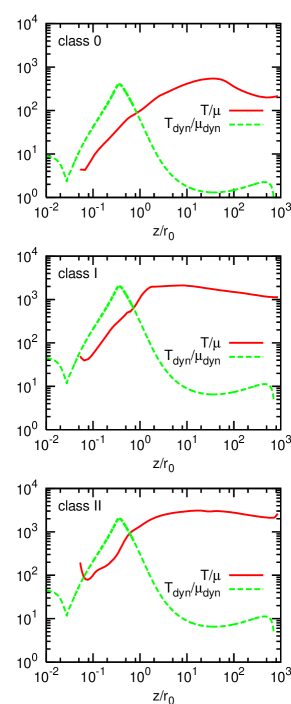
Figure 13: Comparison of $T/\mu$ (in K) as calculated from the heating/cooling terms in our thermal-chemical models (red solid curves) with the same ratio as assumed in the dynamical MHD solutions of Casse & Ferreira (2000), in dashed green, for the 1 AU streamline and 3 stars of differing accretion properties. Note that in the dynamical solution, $T_{\rm dyn}$ is calculated assuming a fully ionised gas, with $\mu_{\rm dyn}=0.5$. A color version of this figure is available in the on-line edition of this journal.

The MHD solution adopted in the present work has been obtained with a prescribed self-similar enthalpy injection function peaking near the disk surface, representing a tiny fraction $f=8\times 10^{-4}$ of the accretion power (Casse & Ferreira 2000). This small surface heating is sufficient to obtain denser, slower disk winds with mass fluxes and poloidal and rotation speeds consistent with observations (see Section 2.1), but the nature of the heating process is not yet identified.

In this context, it is interesting to compare the thermal pressure assumed in the underlying MHD accretion-ejection solution with that obtained from our thermal-chemical calculations where the various known heating, cooling and chemical processes are taken into account. Since the gas density $\rho$ is prescribed by the solution, the relevant quantity to compare thermal pressures is just the ratio $T/\mu$ (with $\mu$ being the mean molecular weight). This comparison is shown in Figure 13 along a 1 AU streamline for our Class 0, Class I, and Class II models.

The value of $T_{\rm dyn}/\mu_{\rm dyn}$ in the dynamical solution first undergoes an increase from the disc surface at $z=h=0.03r_{0}$ to about $z_{t}=10h$ and then an adiabatic decrease. Although the initial rise is not exactly followed by our calculations, it is interesting that the difference between the two curves is less than a factor 2 near the slow magnetosonic point (our starting integration point for the thermo-chemistry). This suggests that the warm gas surface temperatures required to load dense, slow MHD disk winds compatible with observational constraints might be naturally achievable under a wide range of accretion rates, especially as MHD ”turbulent/wave” heating will take place in the deeper resistive disk layers, and wind mass-loading could be further enhanced via upward motions induced by MRI turbulence (Suzuki & Inutsuka 2009).

The discrepancy between computed and assumed $T/\mu$ can exceed a factor 10 at $z_{t}=10h$, and a factor 100 beyond. This discrepancy has however no relevant impact on the dynamical behavior of the solution. Indeed, at $z_{t}$, the ratio of plasma pressure to magnetic pressure in the dynamical solution is already down to only a few $10^{-3}$, so even a large discrepancy in thermal pressure will not affect the wind dynamics. Although the thermal pressure gradient did play an important role in the mass loading (done within the resistive MHD disk layers), it plays no role in the jet acceleration and collimation itself which is mainly due to magnetic forces. Thermal pressure gradients will eventually start affecting the jet dynamics after the jet refocusses towards the axis. For this reason we have not extended our thermal-chemical calculations beyond the recollimation point of the MHD solution.