Abstract

With its three independent parameters, the $ABCD$ matrix serves as the beam transfer matrix in optics. If it is transformed to an equi-diagonal form, the matrix has only two independent parameters determined by optical devices. It is shown that this two-parameter mathematical device contains enough information to describe the basic space-time symmetry of elementary particles. If its trace is smaller than two, this matrix can represent the internal space-time symmetry of massive particles. If equal to two, the matrix is of massless particles. If the trace is greater than two, this matrix describes imaginary-mass particles. This matrix speaks Einstein’s language for space-time structure of elementary particles. As for the optical devices, the laser cavity and the multilayer system are discussed as illustrative physical examples.

1 Introduction

The $ABCD$ matrix is a two-by-two matrix with real elements, and its determinant is one. There are therefore three independent parameters. These elements are determined by optical materials and how they are arranged. The purpose of this note is to explore its mathematical properties which can address more fundamental issues in physics.

First of all, the trace of this matrix could be less than two, equal to two, or greater than two. We are interested in what physical conclusions we can derive from these numbers.

In order to bring the $ABCD$ matrix to the form which will address some fundamental issues in physics, we should first transform it into the equi-diagonal form where the two-diagonal elements are equal to each other [1, 2]. We can achieve this goal by a similarity transformation with a one-parameter matrix. This transformation does not change the trace, and the resulting equi-diagonal matrix has two independent parameters.

We shall call this equi-diagonal matrix the core of the $ABCD$ matrix, and use the notation $[ABCD]$. This matrix cannot always be diagonalized. This creates a non-trivial problem. We shall examine how optical devices, especially periodic systems, can lead us to a better understanding of the problem. For this purpose, we discuss laser cavities and multilayer systems in detail.

If the trace is less than two, the core can be written as

$$[ABCD]=\pmatrix{\cos(\gamma/2)&-e^{\eta}\sin(\gamma/2)\cr e^{-\eta}\sin(\gamma/2)&\cos(\gamma/2)}.$$ (1)

The diagonal elements are equal and smaller than one.

If the trace is greater than two, the $[ABCD]$ matrix takes the form

$$[ABCD]=\pmatrix{\cosh(\gamma/2)&e^{\eta}\sinh(\gamma/2)\cr e^{-\eta}\sinh(\gamma/2)&\cosh(\gamma/2)}.$$ (2)

Here again the diagonal elements are equal, but they are greater than one.

If the trace is equal to two, the core matrix becomes

$$[ABCD]=\pmatrix{1&-\gamma\cr 0&1}.$$ (3)

This matrix also has the same diagonal element, and they are equal to one.

This triangular matrix of Eq.(3) cannot be diagonalized. The core matrices of Eq.(1) and Eq.(2) can be diagonalized, but not by rotation alone. These mathematical subtleties are not well known. The purpose of this report is to show how much physics we can extract from these mathematical details.

The mathematics of group theory allows us to write down a four-by-four Lorentz-transformation matrix for every two-by-two matrix discussed in this paper. In this way, the three matrices given in Eq.(1), and Eq.(2), and Eq.(3) lead to the internal space-time symmetries of elementary particles. They respectively correspond to the symmetries of massive, imaginary-mass, and massless particles respectively [3].

In Sec. 2, we write the $[ABCD]$ matrix in terms of the its generators, and decompose it to three matrices in the form of similarity transformation. It is noted that there is another mathematical device known as the Bargmann decomposition [4]. This decomposition is not a similarity transformation, but it can play other important roles in understanding the $ABCD$ matrix.

In Sec. 3, we discuss a laser cavity as a physical example of the mathematical details of the $[ABCD]$ matrix. In Sec. 4, a multilayer system is discussed as a physical example leading to the desired similarity transformation. The Bargmann decomposition plays the key role in this problem. In Sec. 5, we shall discuss the space-time symmetries implied by the properties of the $[ABCD]$ matrix. The Bargmann decomposition, as well the similarity decompositions, is explained in terms of the Lorentz transformations which leave the momentum of a given particle invariant. Thus, these transformations are applicable to internal space-time symmetries.

2 Decomposition of the ABCD Matrix

We are interested in writing the three different forms of the core matrix in one expression.

$$[ABCD]=\exp{\left\{\frac{1}{2}\pmatrix{0&-x-y\cr x-y&0}\right\}},$$ (4)

where the parameters $x$ and $y$ are determined by the optical materials and how they are arranged. The exponent of this matrix becomes

$$\frac{1}{2}\pmatrix{0&-x-y\cr x-y&0}.$$ (5)

If $x>y$, the matrix becomes

$$\frac{\gamma}{2}\pmatrix{0&-\exp{(\eta/2)}\cr\exp{(-\eta/2)}&0},$$ (6)

which leads to the core matrix of Eq.(1) with

$$\gamma=\sqrt{x^{2}-y^{2}},$$

$$e^{\eta}=\sqrt{\frac{x+y}{x-y}}.$$ (7)

The core matrix $[ABCD]$ can be written as a similarity transformation

$$[ABCD]=B(\eta)R(\theta)B(-\eta)$$ (8)

with

$$B(\eta)=\pmatrix{e^{\eta/2}&0\cr 0&e^{-\eta/2}}$$

$$R(\theta)=\pmatrix{\cos(\theta/2)&-\sin(\theta/2)\cr\sin(\theta/2)&\cos(\theta/2)},$$ (9)

where $\gamma$ is now replaced by the rotation angle $\theta$. $R(\theta)$ is a rotation matrix, and $B(\eta)$ is a squeeze matrix.

If $x<y$, the exponent becomes

$$\frac{\gamma}{2}\pmatrix{0&\exp{(\eta/2)}\cr\exp{(-\eta/2)}&0},$$ (10)

leading to the core matrix of Eq.(2), with

$$\gamma=\sqrt{y^{2}-x^{2}},$$

$$e^{\eta}=\sqrt{\frac{x+y}{y-x}}.$$ (11)

The $[ABCD]$ matrix can now be decomposed into a similarity transformation

$$[ABCD]=B(\eta)S(-\lambda)B(-\eta),$$ (12)

with

$$S(\lambda)=\pmatrix{\cosh(\lambda/2)&\sinh(\lambda/2)\cr\sin(\lambda/2)&\cosh(\lambda/2)},$$ (13)

where $\gamma$ is replaced by the boost parameter $\lambda$. The matrix $B(\eta)$ takes the diagonal form given in Eq.(8) with $\eta$ defined in Eq.(2). $S(\lambda)$ is a squeeze matrix.

If $x=y$, the exponent becomes

$$\pmatrix{1&-x\cr 0&1},$$ (14)

with $x=y=\gamma$.

We now have combined three different expressions for the core of the $ABCD$ matrix into one exponential form of Eq.(4). This form can be decomposed into three matrices constituting a similarity transformation. We shall call this the “Wigner decomposition” for the reasons given in Sec. 5.

There is another form of decomposition known as the Bargmann decomposition [4], which states that the core of the $ABCD$ matrix can be written as

$$[ABCD]=R(\alpha)S(-2\chi)R(\alpha),$$ (15)

where the forms of the rotation matrix $R$ and the squeeze matrix $S$ are given in Eq.(8) and Eq.(2) respectively. If we carry out the matrix multiplication, the $[ABCD]$ matrix becomes

$$\pmatrix{(\cosh\chi)\cos\alpha&-\sinh\chi-(\cosh\chi)\sin\alpha\cr-\sinh\chi+(\cosh\chi)\sin\alpha&(\cosh\chi)\cos\alpha}.$$ (16)

This matrix also has two independent parameters $\alpha$ and $\chi$. We can write these parameters in terms of $\gamma$ and $\eta$ by comparing the matrix elements. For instance, if $x>y$, the diagonal elements lead to

$$\cos(\theta/2)=(\cosh\chi)\cos\alpha.$$ (17)

The off-diagonal elements lead to

$$e^{2\eta}=\frac{(cosh\chi)\sin\alpha+\sinh\chi}{(cosh\chi)\sin\alpha-\sinh\chi}$$ (18)

As for physical applications, let us consider periodic systems, such as laser cavities and multilayer systems. The exponential form given in Eq.(4) tells us that it is a matter of replacing the $\gamma$ parameter by $N\gamma$ for N repeated applications [2]. Let us see some examples.

3 Laser Cavities

As the first example, let us consider the laser cavity consisting of two identical concave mirrors separated by a distance $d$. Then the $ABCD$ matrix for a round trip of one beam is

$$\pmatrix{1&0\cr-2/R&1}\pmatrix{1&d\cr 0&1}\pmatrix{1&0\cr-2/R&1}\pmatrix{1&d\cr 0&1},$$ (19)

where the matrices

$$\pmatrix{1&0\cr-2/R&1},\quad\pmatrix{1&d\cr 0&1}$$ (20)

are the mirror and translation matrices respectively. The parameters $R$ and $d$ are the radius of the mirror and the mirror separation respectively. This form is quite familiar to us from the laser literature [5, 6, 7, 8].

However, the crucial question is what happens when this process is repeated. We are thus led to the question of whether the chain of matrices in Eq.(19) can be brought to an equi-diagonal form and eventually to a form of the Wigner decomposition. We are interested in finding the core of Eq.(19). For his purpose, we rewrite the matrix of Eq.(19) as

$$\pmatrix{1&-d/2\cr 0&1}\pmatrix{1&d/2\cr 0&1}\pmatrix{1&0\cr-2/R&1}\pmatrix{1&d/2\cr 0&1}^{2}$$

$$\times\pmatrix{1&0\cr-2/R&1}\pmatrix{1&d/2\cr 0&1}\pmatrix{1&d/2\cr 0&1}.$$ (21)

In this way, we translate the system by $-d/2$ using a translation matrix given in Eq.(20), and write the $ABCD$ matrix of Eq.(19) as

$$\pmatrix{1&-d/2\cr 0&1}\left[\pmatrix{1-d/R&d-d^{2}/2R\cr-2/R&1-d/R}\right]^{2}\pmatrix{1&d/2\cr 0&1}.$$ (22)

We are thus led to concentrate on the matrix in the middle

$$\pmatrix{1-d/R&d-d^{2}/2R\cr-2/R&1-d/R},$$ (23)

which can be written as

$$\pmatrix{\sqrt{d}&0\cr 0&1/\sqrt{d}}\pmatrix{1-d/R&1-d/2R\cr-2d/R&1-d/R}\pmatrix{1/\sqrt{d}&0\cr 0&\sqrt{d}}.$$ (24)

It is then possible to decompose the $ABCD$ matrix into

$$E~{}C^{2}~{}E^{-1},$$ (25)

with

$$C=\pmatrix{1-d/R&1-d/2R\cr-2d/R&1-d/R},$$

$$E=\pmatrix{1&-d/2\cr 0&1}\pmatrix{\sqrt{d}&0\cr 0&1/\sqrt{d}}.$$ (26)

The $C$ matrix now contains only dimensionless numbers, and it can be written as

$$C=\pmatrix{\cos(\gamma/2)&e^{\eta}\sin(\gamma/2)\cr-e^{-\eta}\sin(\gamma/2)&\cos(\gamma/2)},$$ (27)

with

$$\cos(\gamma/2)=1-\frac{d}{R},$$

$$e^{\eta}=\sqrt{\frac{2R-d}{4d}}$$ (28)

Here both $d$ and $R$ are positive, and the restriction on them is that $d$ be smaller than $2R$. This is the stability condition frequently mentioned in the literature [6, 7].

Thus, the $[ABCD]$ core matrix is $C^{2}$, and takes the form

$$[ABCD]=\pmatrix{\cos(\gamma)&e^{\eta}\sin(\gamma)\cr-e^{-\eta}\sin(\gamma)&\cos(\gamma)},$$ (29)

and the similarity transformation which connects this core matrix with the original $ABCD$ matrix of Eq.(19) is the matrix $E$ given in Eq.(3).

4 Multilayer Optics

We consider an optical beam going through a periodic medium with two different refractive indexes. If the beam traveling in the first medium hits the second medium, it is partially transmitted and partially reflected. In order to maintain the continuity in the pointing picture, we normalize the electric field as

$$E_{1}^{(\pm)}=\frac{1}{\sqrt{n_{1}}}\exp{\left({\pm}ik_{1}z-\omega t\right)}$$

$$E_{2}^{(+)}=\frac{1}{\sqrt{n_{2}}}\exp{\left({\pm}ik_{2}z-\omega t\right)}$$ (30)

for the optical beams in the first and second media respectively. The superscript $(+)$ and $(-)$ are for the incoming and reflected rays respectively.

These two optical rays are related by the two-by-two $ABCD$ matrix, according to

$$\pmatrix{E_{2}^{(+)}\cr E_{2}^{(-)}}=\pmatrix{A&B\cr C&D}\pmatrix{E_{1}^{(+)}\cr E_{1}^{(-)}}.$$ (31)

Of course the elements of this matrix are determined by transmission coefficients as well as the phase shifts the beams experience while going through the media [9].

When the beam goes through the first medium to the second, we may use the boundary matrix[11]

$$Q(\sigma)=\pmatrix{\cosh(\sigma/2)&\sinh(\sigma/2)\cr\sinh(\sigma/2)&\cosh(\sigma/2)},$$ (32)

where the parameter $\sigma$ is determined by the reflection and the transmission coefficients [8, 9, 11]. Then the boundary matrix for the beam going from the second medium should be $Q(-\sigma)$.

In addition, we have to consider the phase shifts the beams have to go through. When the beam goes trough the first media, we can use the phase-shift matrix

$$P\left(\delta_{1}\right)=\pmatrix{e^{-i\delta_{1}/2}&0\cr 0&e^{i\delta_{1}/2}},$$ (33)

and a similar expression for $P\left(\delta_{2}\right)$ for the second medium.

We are thus led to consider one complete cycle starting from the midpoint of the second medium, and write

$$P\left(\delta_{2}/2\right)Q(\sigma)P\left(\delta_{1}\right)Q(-\sigma)P\left(\delta_{2}/2\right).$$ (34)

If multiplied into one matrix, is this matrix equi-diagonal to accept the Wigner and Bargmann decompositions? Another question is whether the matrices in the above expression can be converted into matrices with real element.

In order to answer the second question, let us consider the similarity transformation

$$C_{1}~{}P(\delta)Q(\sigma)~{}C_{1}^{-1},$$ (35)

with

$$C_{1}={1\over\sqrt{2}}\pmatrix{1&i\cr i&1}.$$ (36)

This transformation leads to

$$R(\delta)Q(\sigma),$$ (37)

where

$$R(\delta)=\pmatrix{\cos(\delta/2)&-\sin(\delta/2)\cr\sin(\delta/2)&\cos(\delta/2)}.$$ (38)

This notation is consistent with the rotation matrices used in Sec. 2.

Let us make another similarity transformation with

$$C_{2}={1\over\sqrt{2}}\pmatrix{1&1\cr-1&1}.$$ (39)

This changes $Q(\sigma)$ into $B(\sigma)$ without changing $R(\delta)$, where

$$B(\sigma)=\pmatrix{e^{\sigma/2}&0\cr 0&e^{-\sigma/2}},$$ (40)

again consistent with the $B(\eta)$ matrix used in Sec. 2.

Thus the net similarity transformation matrix is [10]

$$C=C_{2}C_{1}={1\over\sqrt{2}}\pmatrix{e^{i\pi/4}&e^{i\pi/4}\cr-e^{-i\pi/4}&e^{-i\pi/4}},$$ (41)

with

$$C^{-1}={1\over\sqrt{2}}\pmatrix{e^{-i\pi/4}&-e^{i\pi/4}\cr e^{-i\pi/4}&e^{i\pi/4}}.$$ (42)

If we apply this similarity transformation to the long matrix chain of Eq.(34), it becomes another chain

$$M=R\left(\delta_{2}/2\right)B(\sigma)R\left(\delta_{1}\right)B(-\sigma)R\left(\delta_{2}/2\right),$$ (43)

where all the matrices are real.

Let us now address the main question of whether this matrix chain can be brought to one equi-diagonal matrix. We note first that the three middle matrices can be written in a familiar form

$$M=B(\sigma)R\left(\delta_{1}\right)B(-\sigma)$$

$$=\pmatrix{\cos(\delta_{1}/2)&-e^{\sigma}\sin(\delta_{1}/2)\cr e^{-\sigma}\sin(\delta_{1}/2)&\cos(\delta_{1}/2)}.$$ (44)

However, due to the rotation matrix $R\left(\delta_{2}/2\right)$ at the beginning and at the end of Eq.(43), it is not clear whether the entire chain can be written as a similarity transformation.

In order to resolve this issue, let us write Eq.(4) as a Bargmann decomposition

$$R(\alpha)S(-2\chi)R(\alpha),$$ (45)

with its explicit expression given in Eq.(16). The parameters $\alpha$ and $\chi$ are related to $\sigma$ and $\delta_{1}$ by

$$\cos(\delta_{1}/2)=(\cosh\chi)\cos\alpha,$$

$$e^{2\sigma}=\frac{(cosh\chi)\sin\alpha+\sinh\chi}{(cosh\chi)\sin\alpha-\sinh\chi}.$$ (46)

It is now clear that the entire chain of Eq.(34) can be written as another Bargmann decomposition

$$M=R(\alpha+\delta_{2}/2)S(-2\chi)R(\alpha+\delta_{2}/2).$$ (47)

Finally, if the trace of this matrix is less than two, it can be converted to a Wigner decomposition

$$M=B(\eta)R(\theta)B(-\eta)$$ (48)

with

$$\cos(\theta/2)=(\cosh\chi)\cos(\alpha+\delta_{2}/2),$$

$$e^{2\eta}=\frac{(\cosh\chi)\sin(\alpha+\delta_{2}/2)+\sinh\chi}{(\cosh\chi)\sin(\alpha+\delta_{2}/2)-\sinh\chi}.$$ (49)

Similar expressions can be derived for other values of the trace [12].

It is interesting to note that the Bargmann decomposition plays an essential role in bringing the chain of five matrices given in Eq.(43) to the Wigner decomposition of Eq.(48) consisting three matrices. We shall see what other function the Bargmann decomposition can perform in Sec. 5.

5 Space-time Symmetries

These properties are applicable to many other branches of physics. For instance, one of the persisting problems is the internal space-time symmetry of elementary particles in Einstein’s Lorentz-covariant world.

The mathematics of group theory allows us to translate the rotation and squeeze matrices of Eq.(8) and Eq.(2) into the following four-by-four matrices respectively.

$$R(\theta)=\pmatrix{\cos\theta&0&\sin\theta&0\cr 0&1&0&0\cr-\sin\theta&0&\cos\theta&0\cr 0&0&0&1},$$

$$S(\lambda)=\pmatrix{\cosh\lambda&0&0&\sinh\lambda\cr 0&1&0&0\cr 0&0&1&0\cr\sinh\lambda&0&0&\cosh\lambda},$$

$$B(\eta)=\pmatrix{1&0&0&0\cr 0&1&0&0\cr 0&0&\cosh\eta&\sinh\eta\cr 0&0&\sinh\eta&\cosh\eta},$$ (50)

They are applicable to the Minkowskian four-vector $(x,y,z,t)$. The $R(\theta)$ matrix performs a rotation around the $y$ axis, and $S(\lambda)$ is for Lorentz boosts along the $x$ axis. The $B(\eta)$ matrix boosts the system along the $z$ direction.

Together with a rotation matrix around $z$ axis

$$\ Z(\phi)=\pmatrix{\cos\phi&-\sin\phi&0&0\cr\sin\phi&\cos\phi&0&0\cr 0&0&1&0\cr 0&0&0&1},$$ (51)

they constitute Wigner’s little groups dictating internal space-time symmetries of massive and imaginary-mass particles [3]. The triangular matrix of Eq.(3) leads to the little group for massless particles. The little groups are the subgroups of the Lorentz group whose transformations leave the four-momentum of a given particle invariant.

Let us go back to Eq.(1) which, according to Eq.(8), can be decomposed to a similarity transformation

$$W(\eta,\theta)=B(\eta)R(\theta)B(-\eta).$$ (52)

We can write this decomposition with the four-by four matrices given in in Eq.(5).

Let us then consider a massive particle moving along the $z$ direction with the velocity parameter $v/c=\tanh\eta$, and its four-momentum

$$(0,0,m\sinh\eta,m\cosh\eta),$$ (53)

where $m$ is the mass of the particle.

We can boost this particle using the boost matrix $B(-\eta)$, which is the inverse of the four-by-four matrix given in Eq.(5). The particle becomes at rest, with its four-momentum

$$(0,0,0,m),$$ (54)

and with zero velocity. The rotation matrix $R(\theta)$ rotates this particle without changing its momentum. During this process, the particle changes the direction of its spin. Finally, $B(\eta)$ boosts the particle and restores its momentum, as is illustrated in Fig. 1. Thus, it is appropriate to call the form of Eq.(52) the Wigner decomposition. In this way, the four-by-four expression for Eq.(8) changes the internal space-time structure of the particle.

The essential function of the Wigner decomposition is to provide the subgroup of the Lorentz group which will leave the given four-momentum of a particle invariant [3].

The Bargmann decomposition also provides momentum-preserving transformations. The decomposition consists of a rotation, a boost, and another rotation as illustrated in Fig. 1. It is interesting to note that the Wigner decomposition and the Bargmann decomposition can serve the same purpose of providing a Lorentz transformation which leaves the momentum invariant.

One key question from this table is what happens to the $O(3)$-like little group when the particle momentum becomes infinity or its mass becomes zero. The question is whether the little group for a massive particles becomes that for a massless particle. The answer to this question is Yes, but this issue had a stormy history before this definitive answer [13]. Indeed, when $\eta$ becomes infinity, the four-by-four form of Eq(52) becomes

$$\pmatrix{1&0&-\gamma&\gamma\cr 0&1&0&0\cr\gamma&0&1-\gamma^{2}/2&\gamma^{2}/2\cr\gamma&0&-\gamma^{2}/2&1+\gamma^{2}/2}.$$ (55)

When applied to the momentum of a massless particle moving in the negative $z$ direction with

$$(0,0,p,p),$$ (56)

This matrix leaves the above four-momentum invariant, but it performs a gauge transformation [13]. This aspect of Wigner’s little group is illustrated in Table 1.

         

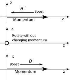
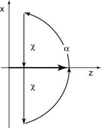
Figure 1: Wigner decomposition (left) and Bargmann decomposition (right). These figures illustrate momentum preserving transformations. In the Wigner transformation, a massive particle is brought to its rest frame. It can be rotated while the momentum remains the same. This particle is then boosted back to the frame with its original momentum. In the Bargmann decomposition, the momentum is rotated, boosted, and rotated to its original position.

Table 1: Massive and massless particles in one package. Einstein unified the energy-momentum relation for slow (massive) and fast (massless) particles with one Lorentz-covariant formula. Likewise, Wigner’s little group unifies the internal space-time symmetries of particles. When boosted, the spin along the direction remains invariant. This is called the Lorentz-invariant helicity. The spins along the transverse directions collapse into a gauge degree of freedom in the infinite-momentum or zero-mass limit [13, 14].

	Massive	Lorentz	Massless
	Slow	Covariance	Fast
Energy-	$E=$	Einstein’s
Momentum	$p^{2}/2m$	$E=[p^{2}+m^{2}]^{1/2}$	$E=p$
Internal	$S_{3}$	Wigner’s	$S_{3}$
Symmetries	$S_{1},S_{2}$	Little Group	Gauge Trans.

Concluding Remarks

In this report, we have discussed some properties of the $ABCD$ matrix which serves as the standard research tool in ray optics. This two-by-two matrix four real elements, but only three independent parameters if the determinant of the matrix is constrained to be one.

If the determinant is restricted to be one, the $ABCD$ matrix has three independent parameters. It was noted that this matrix can be written as a similarity transformation of a core matrix with two independent parameters. Two physical examples are given to illustrate how these parameters are determined from optical devices.

It is remarkable that this two-parameter matrix contains enough information to describe the internal space-time structure of elementary particles.

References

- [1] S. Baskal and Y. S. Kim, J. Opt. Soc. Am. A 26, 3049 (2009).
- [2] S. Baskal and Y. S. Kim, J. Mod. Opt. [57], 1251 (2010).
- [3] E. Wigner, Ann. Math. 40, 149 (1939); Y. S. Kim and M. E. Noz, Theory and Applications of the Poincaré Group (Reidel, Dordrecht, 1986).
- [4] V. Bargmann, Ann. Math. 48, 568 (1947).
- [5] A. Yariv, Quantum Electronics (Wiley, New York, 1975).
- [6] H. A. Haus, Waves and Fields in Optoelectronics (Prentice-Hall, Englewood Cliffs, New Jersey, 1984).
- [7] J. Hawkes and I. Latimer, Lasers: Theory and Practice (Prentice-Hall, New York, 1995).
- [8] B. E. A. Saleh and M. C. Teich, Fundamentals of Photonics, Second Edition (Wiley, Hoboken, New Jesey, 2007).
- [9] R. A. M. Azzam and I. Bashara, Ellipsometry and Polarized Light (North-Holland, Amsterdam, 1977).
- [10] E. Georgieva and Y. S. Kim, Phys. Rev. E 64, 026602 (2001).
- [11] J. J. Monzón and L. L. Sánchez-Soto, J. Opt. Soc. Am. A 17, 1475 (2000).
- [12] E. Georgieva and Y. S. Kim, Phys. Rev. E 68, 026606 (2003).
- [13] Y. S. Kim and E. P. Wigner, J. Math. Phys. 31, 55 (1990).
- [14] D. Han, Y. S. Kim, and D. Son, J. Math. Phys. 27, 2228 (1986).