Spatially explicit models for inference about density in unmarked or partially marked populations

Abstract

Recently developed spatial capture–recapture (SCR) models represent a major advance over traditional capture–recapture (CR) models because they yield explicit estimates of animal density instead of population size within an unknown area. Furthermore, unlike nonspatial CR methods, SCR models account for heterogeneity in capture probability arising from the juxtaposition of animal activity centers and sample locations. Although the utility of SCR methods is gaining recognition, the requirement that all individuals can be uniquely identified excludes their use in many contexts. In this paper, we develop models for situations in which individual recognition is not possible, thereby allowing SCR concepts to be applied in studies of unmarked or partially marked populations. The data required for our model are spatially referenced counts made on one or more sample occasions at a collection of closely spaced sample units such that individuals can be encountered at multiple locations. Our approach includes a spatial point process for the animal activity centers and uses the spatial correlation in counts as information about the number and location of the activity centers. Camera-traps, hair snares, track plates, sound recordings, and even point counts can yield spatially correlated count data, and thus our model is widely applicable. A simulation study demonstrated that while the posterior mean exhibits frequentist bias on the order of 5–10% in small samples, the posterior mode is an accurate point estimator as long as adequate spatial correlation is present. Marking a subset of the population substantially increases posterior precision and is recommended whenever possible. We applied our model to avian point count data collected on an unmarked population of the northern parula (Parula americana) and obtained a density estimate (posterior mode) of 0.38 (95% CI: 0.19–1.64) birds/ha. Our paper challenges sampling and analytical conventions in ecology by demonstrating that neither spatial independence nor individual recognition is needed to estimate population density—rather, spatial dependence can be informative about individual distribution and density.

copyrightownerIn the Public Domain

and

t1Supported by the North American Breeding Bird Survey Program.

1 Introduction

Estimates of population density are required in basic and applied ecological research, but are difficult to obtain for many species, including some of the most critically endangered. A primary obstacle faced when estimating population density is that the number of individuals captured or detected is an unknown fraction of the actual number present, $N$. Traditional capture–recapture (CR) methods [Seber (1973)] yield estimates of $N$; however, the effective area sampled is typically unknown, and thus density cannot be explicitly estimated [Dice (1938), Wilson and Anderson (1985)]. This is a well-known deficiency of traditional CR methods that makes it difficult to interpret differences in abundance among sampling locations and hence test hypotheses regarding spatial variation in abundance.

An additional limitation of nonspatial CR methods is that, even if effective sample area is known, estimators of $N$ can be biased by unmodeled heterogeneity in capture probability resulting from the distance between animal “activity centers” and survey locations. The definition of an activity center will depend upon the biology of the species, but often it can be regarded as the centroid of an animal’s home range or, more generally, the first spatial moment of an animal’s locations during some time interval. Intuitively, individuals with activity centers close to a trap are more likely to be captured than individuals whose activity centers are further away. Spatial capture–recapture (SCR) models [Efford (2004), Borchers and Efford (2008), Royle and Young (2008), Royle et al. (2009)] produce direct estimates of density or population size for explicit spatial regions by asserting a spatial point process model for the activity centers, and modeling capture probability as a function of the distance between the survey locations and the activity centers. Although the activity centers cannot be directly observed, information about their locations comes from the spatial coordinates of the traps where individuals are captured—data which have always been available but were rarely utilized until recently.

Because SCR models overcome the limitations of CR methods without requiring additional data, they represent a major advance in efforts to estimate population density, and their use is becoming widespread [Dawson and Efford (2009), Efford, Dawson and Borchers (2009), Gardner, Royle and Wegan (2009), Sollmann et al. (2011), Gopalaswamy et al. (2012)]. However, use of such methods requires that all individuals are uniquely identifiable, which can be difficult to achieve in practice. In some cases, it is not even possible to identify individuals, such as in avian point count surveys, which involve counting unmarked individuals from multiple points within a study area. In other cases, even when resources are available to obtain individual recognition, the identity of many individuals often remains unknown. For example, in camera trapping studies [O’Connell, Nichols and Karanth (2011)], the resulting photographs are not always sufficient for identification due to similar markings among animals. For some species, no natural markings are present to aid recognition (e.g., fisher Martes pennanti, coyote Canis latrans), and physically capturing individuals may be too difficult or intrusive.

In this paper, we present a model allowing for inference about density and population size when individuals cannot be uniquely identified nor detected with certainty. Our model requires spatially correlated count data from sample locations in close proximity to one another such that individuals can be detected at multiple locations. Rather than viewing the spatial correlation as an inferential obstacle, we utilize the correlation as information about distribution and population size. We develop our model by regarding the encounter frequencies for each individual, or for a subset of individuals, as latent or missing data, and we provide a Bayesian analysis of the model based on Markov chain Monte Carlo (MCMC). We demonstrate efficacy of the approach using a simulation study, and we present an application in which bird density is estimated from standard point count data.

Our paper challenges two common assertions in statistical ecology: first is that sample units should be structured so as to ensure independence of the observable random variable and second is that individual information is needed to obtain estimates of population size and density. Our proposed model directly refutes both claims and suggests new classes of sampling designs and statistical models for making inferences about animal demographic parameters.

2 Sampling design and data

We consider a sampling design in which animals are counted at $J$ traps on $K$ occasions. Although we use the term “trap,” anything capable of recording counts of unmarked individuals could be used, such as a camera or a human observer conducting a point count survey. The sample occasion can be an arbitrary time period, such as a single day in a camera trap study, or a 10 min survey interval. Trap locations are characterized by the coordinates, $\mathbf{X}=\{\mathbf{x}_{j}\}\in\mathbb{R}^{2}$ for $j=1,2,\ldots,J$. The data resulting from this design are the $J\times K$ matrix of counts, $\mathbf{n}=\{n_{jk}\};k=1,2,\ldots,K$.

Unlike similar count-based sampling protocols, this design aims to induce correlation in the neighboring counts by organizing the traps sufficiently close together so that individual animals might be encountered at multiple locations. Thus, we do not make the customary assumptions that counts can be viewed as i.i.d. outcomes and that no movement occurs between sampling occasions. In the following sections we develop a hierarchical model that describes the process by which such correlation is induced and, by fitting this model to data, we obtain estimates of density and related parameters.

3 The hierarchical model

3.1 Data model

The data consist of the trap-specific counts ${\mathbf{n}}$ and the trap coordinates $\mathbf{X}$. The count data can be viewed as reduced information summaries of the data that would be observed if all individuals in the population were marked or otherwise distinguishable. Let $z_{ijk}$ represent the encounter data for individual $i=1,\ldots,N$ at trap $j$ on occasion $k$. If an individual can be detected at most once during a sampling occasion, $z_{ijk}$ will be binary, or if individuals can be detected multiple times during a single occasion, $z_{ijk}\geq 0$ is an integer. In standard capture–recapture studies, $z_{ijk}$ is observed directly for captured individuals, and the collection of observations for an individual is referred to as its “encounter history.” The encounter data are deterministically related to the trap-level count data according to

$$n_{jk}=\sum_{i=1}^{N}z_{ijk}.$$

However, we do not know $N$, and we cannot observe $z_{ijk}$ when individuals are unmarked. Nonetheless, by developing our model in terms of these missing data, a simplified analysis of the posterior is possible using classical data augmentation methods. In particular, sampling the latent data $\mathbf{z}_{jk}=\{z_{1jk},z_{2jk},\ldots,z_{Njk}\}$, conditional on $n_{jk}$, uses an application of data augmentation [Tanner and Wong (1987)] similar to that employed by Wolpert and Ickstadt (1998). We will temporarily proceed by assuming that $N$ is known so that we can focus on the detection process.

For the latent encounter data we assume

$$z_{ijk}\sim\operatorname{Poisson}(\lambda_{ij}),$$ (1)

where $\mathbb{E}(z_{ijk})=\lambda_{ij}$ is the expected number of captures or detections of individual $i$ at trap $j$. We model this encounter rate as a function of the Euclidean distance between the individual’s activity center $\mathbf{s}_{i}$ (also a latent variable) and the trap location, $d_{ij}=\|\mathbf{s}_{i}-\mathbf{x}_{j}\|$. A model for the activity centers is presented in the next section; here we continue by assuming that the expected encounter frequency of an individual is related to $d_{ij}$ as follows:

$$\lambda_{ij}=\lambda_{0}g(d_{ij}),$$

where $\lambda_{0}$ is the encounter rate at $d=0$ and $g(d)$ is a positive-valued, typically monotonically decreasing, function of distance. We make use of the standard half-normal detection function used in distance sampling [Buckland et al. (2001)]:

$$g(d)=\exp\bigl{(}-d^{2}/2\sigma^{2}\bigr{)},$$

where $\sigma$ is a scale parameter determining the rate of decay in encounter probability. This parameter also determines the degree of correlation among counts since animals with large home ranges are more likely to be detected at multiple traps relative to animals with small home ranges. This is analogous to correlation induced by averaging spatial noise, in which case there is a well-defined relationship between the smoothing kernel and the induced covariance function [Higdon (2002)]. Finally, we note that although our focus here is on distance-related heterogeneity in encounter rate, other sources of variation could be modeled by considering trap- or occasion-specific covariates of $\lambda_{0}$ and $\sigma$ as is customary in traditional SCR applications.

Under this formulation of the model based on data augmentation—that is, including the latent encounter data in the model—the full conditional of the latent encounter data is multinomial

$$\{z_{1jk},z_{2jk},\ldots,z_{Njk}\}\sim\operatorname{MN}\bigl{(}n_{jk},\{\pi_{1j},\pi_{2j},\ldots,\pi_{Nj}\}\bigr{)},$$

where $\pi_{ij}=\lambda_{ij}/\sum_{i}\lambda_{ij}$. A complete description of all the full conditionals is provided in the supplementary material [Chandler and Royle (2013)].

We note that the latent data model implies that the trap counts are also Poisson:

$$n_{jk}\sim\operatorname{Poisson}(\Lambda_{j}),$$ (2)

where

$$\Lambda_{j}=\lambda_{0}\sum_{i=1}^{N}g(d_{ij}),$$

and the analysis can proceed from this model specification without contemplating the latent data. Further, because $\Lambda_{j}$ does not depend on $k$, we can aggregate the replicated counts, by a sufficiency argument, defining $n_{j\cdot}=\sum_{k}n_{jk}$ and then

$$n_{j\cdot}\sim\operatorname{Poisson}(K\Lambda_{j}).$$

As such, $K$ and $\lambda_{0}$ serve equivalent roles as affecting baseline encounter rate. This formulation of the model in terms of the aggregate counts simplifies computations, as the unobserved encounter histories do not need to be updated in the MCMC estimation scheme. However, retaining the latent encounter data in the formulation of the model is important if some individuals are uniquely marked. In this case, modifying the MCMC algorithm to include both types of data is trivial.

3.2 Process model

The models for the data and the latent data are conditional on the underlying ecological process of interest, which is the number and locations of the unobserved activity centers $\{\mathbf{s}_{i}\}$; $i=1,2,\ldots,N$. We view the activity centers as outcomes of a spatial point process within a state-space, or observation window, $\mathcal{S}$, which for simplicity we treat as planar $\cal{S}\subset\mathbb{R}\mathrm{{}^{2}}$. Although any polygon containing $\mathbf{X}$ could be considered, in practice $\mathcal{S}$ should be chosen large enough so that an individual’s encounter rate is negligible if its activity center occurs on the edge of the polygon. This will typically be a function of the species’ home range size. Alternatively, $\mathcal{S}$ may be defined by geographic boundaries, such as when a species occurs on an island; or it may be defined based upon biological considerations such as suitable habitat [Royle et al. (2009)].

In principle, general point process models could be considered [Borchers and Efford (2008), Illian et al. (2008)], but for simplicity we adopt the homogeneous model

$${\mathbf{s}}_{i}\sim\operatorname{Uniform}({\cal S}),$$

which is to say that the point process intensity is constant $\mu(x)_{x\in\mathcal{S}}=N/\nu(\mathcal{S})$ where $\nu(\mathcal{S})$ is the area of the state-space. Under this model, animals can move about their activity centers, but the activity centers themselves do not move. Furthermore, the activity centers are assumed to exhibit no attraction or repulsion—assumptions that might not strictly hold when animals exhibit behaviors such as territoriality. However, the uniform model allows for any realized configuration of activity centers, and, hence, the estimated locations of activity centers may reflect departure from this assumption, albeit implicitly rather than explicitly.

Thus far we have treated $N$ as known, which implies that the model for the activity centers is a binomial point process. Although the model is naturally described conditional on $N$, that is, in terms of $N$ latent encounter histories, in all practical applications $N$ is unknown and, in fact, is the object of inference.

3.3 $N$ unknown

The fact that $N$ is unknown presents a technical challenge when implementing MCMC because the dimension of the parameter space can change with each Monte Carlo iteration, as the number of latent activity centers changes. To resolve this, we expand our data augmentation scheme following Royle, Dorazio and Link (2007) and Royle and Dorazio (2012) who proposed fixing the dimensions of parameter space by contemplating the existence of $M$, rather than $N$ individuals in the population, where $M$ is some integer $\gg N$. This strategy, known as parameter-expanded data augmentation [Liu and Wu (1999)], not only fixes the dimensions of the problem, but it also allows for the specification of a discrete uniform prior $N\sim\operatorname{DUnif}(0,M)$. We construct this prior by assuming $N|M,\psi\sim\operatorname{Bin}(M,\phi)$ and $\phi\sim\operatorname{Unif}(0,1)$ which implies, marginally, that $N$ has the discrete uniform prior. However, the hierarchical formulation of the prior suggests an implementation in which we introduce a set of latent indicator variables $w_{i}\sim\operatorname{Bern}(\psi);i=1,2,\ldots,M$ and, furthermore, the model implies that $z_{ijk}$ is obtained from the specified distribution (1) if $w_{i}=1$. Alternatively, if $w_{i}=0$, then $z_{ijk}=0$ with probability 1. In effect, extending the model in this way induces a reparameterization for the latent counts that is a zero-inflated version of the original conditional-on-$N$ model. Specifically, the model under parameter-expanded data augmentation becomes

$$z_{ijk}|w_{i} \sim \operatorname{Poisson}(\lambda_{ij}w_{i}),$$

$$w_{i} \sim \operatorname{Bern}(\psi)$$

and, hence, $N=\sum_{i=1}^{M}w_{i}$ and population density is simply $D=N/\nu(\mathcal{S})$. In general, $M$ should be large enough such that the posterior of $N$ is unaffected by its choice, that is, $\operatorname{Pr}(N=M)\approx 0$; however, setting $M$ too high will increase computation time unnecessarily.

3.4 The joint posterior distribution

Assuming mutual independence of the hyperpriors, that is, $[\psi,\lambda_{0},\sigma]\propto[\psi][\lambda_{0}][\sigma]$, the joint posterior distribution of the parameters is

$$[\mathbf{z},\mathbf{w},\mathbf{s},\psi,\lambda_{0},\sigma,|\mathbf{n},\mathbf{X}]$$

$$\qquad\propto\Biggl{\{}\prod_{i=1}^{M}\Biggl{\{}\prod_{j=1}^{J}\prod_{k=1}^{K}[n_{jk}|z_{ijk}][z_{ijk}|w_{i},\mathbf{s}_{i},\sigma,\lambda_{0}]\Biggr{\}}[w_{i}|\psi][\mathbf{s}_{i}]\Biggr{\}}[\psi][\lambda_{0}][\sigma].$$

The only distributions not specified thus far are $[\lambda_{0}]$ and $[\sigma]$, which should be chosen to reflect prior knowledge or lack thereof. Examples are presented in Section 4.

We developed two distinct Metropolis-within-Gibbs MCMC algorithms for this model [Chandler and Royle (2013)]. In the first, the missing encounter data are sampled from their full conditionals, which is useful when one or more individual identities are available, in which case the encounter frequencies $\mathbf{z}_{i}$ are observable for those individuals. The second formulation of the algorithm is unconditional on the latent encounter frequencies. In that case, the marginal distribution for $n_{jk}$ is precisely equation (2). This algorithm is more computationally efficient because it avoids having to update the missing $z_{ijk}$ of which there are many. A description of the two algorithms and the full conditionals, along with R code to implement the models, is presented in the supplementary material [Chandler and Royle (2013)].

4 Applications

4.1 Simulation studies

We carried out two simulation studies to evaluate the basic efficacy of the estimator. In the first study, all individuals were unmarked and we assessed posterior properties by simulating replicate data sets under varying degrees of correlation in the counts. In the second study, we measured the improvements in posterior precision obtained by marking a subset of the population.

To investigate the effects of correlation, we used a $15\times 15$ trap grid with unit spacing and simulated scenarios with $\sigma\in\{0.5,0.75,1.0\}$. We selected these values because $\sigma$ should not be too small relative to the grid spacing or the counts are independent, that is, the trap totals are then i.i.d. Poisson random variables. Similarly, $\sigma$ should not be too large relative to trap spacing or else again the counts become i.i.d. Poisson random variables. We note that trap spacing is widely recognized as being relevant in the application of spatial capture–recapture models, where models require observations of individuals at multiple traps, although to this point in time little formal analysis of the design problem has been done. For the other parameters in the model we considered $T\lambda_{0}\in\{2.5,5.0\}$ and $N\in\{27$, $45$, $75$} individuals distributed on a $20\times 20$ unit state-space centered over the $15\times 15$ array of trap locations. This configuration implies a buffer of 3 units around the traps, which was sufficiently large to ensure that encounter rate was negligible for the values of $\sigma$ considered. We fit the model to 200 data sets for each of the 18 scenarios. For each simulation, we drew 32,000 posterior samples and discarded the initial 2000. We then computed root-mean-squared-error (RMSE) for the posterior mean and mode as well as coverage rates for the 95% highest posterior density (HPD) intervals. Because our interest was in the performance of the estimator in specific regions of the parameter space, we emphasize that our evaluation of the estimators is based on a frequentist evaluation of specific posterior features (mean or mode). That is, we fixed the parameters and generated replicate data sets under the specified model and then calculated RMSE by averaging over the data-generating distribution $(\mathrm{data}|\mathrm{parameters})$. Classical notions of Bayesian optimality based on averaging over the posterior distribution therefore do not apply.

Results of our first simulation study indicate that for the small level of $\sigma$, the posterior mode, if regarded as a point estimator of $N$, is approximately frequentist unbiased (Table 1). However, the posterior distributions are skewed, which results in posterior means exhibiting frequentist bias on the order of 5–10%. Substantial reductions in RMSE are realized as effective encounter rate doubles from 2.5 to 5.0 ($T=5$ to $T=10$). Coverage of 95% HPD intervals is close to nominal for this case. Performance of the estimator deteriorates as the ratio of $\sigma$ to trap spacing increases. For $\sigma=0.75$ the posterior distributions are centered approximately over the data generating value (having nearly frequentist unbiased modes), but the coverage is slightly lower than nominal as the posterior becomes more strongly skewed. The general pattern holds for the highest level of $\sigma=1.0$.

=290pt $\bolds{\sigma}$ $\bolds{N}$ $\bolds{T}$ Mean RMSE Mode RMSE Coverage 0.50 27 $5$ $30.0$ $8.12$ $26.9$ $6.77$ 0.965 $10$ $28.9$ $5.39$ $27.3$ $5.14$ 0.970 45 $5$ $50.4$ $13.48$ $45.5$ $11.37$ 0.965 $10$ $47.6$ $8.90$ $45.2$ $8.50$ 0.945 75 $5$ $83.2$ $19.94$ $75.3$ $16.92$ 0.945 $10$ $78.7$ $13.54$ $74.6$ $12.77$ 0.945 0.75 27 $5$ $30.5$ $8.83$ $27.3$ $7.69$ 0.945 $10$ $28.6$ $5.76$ $26.9$ $5.42$ 0.935 45 $5$ $52.6$ $15.63$ $46.6$ $13.95$ 0.950 $10$ $49.5$ $11.38$ $45.9$ $10.91$ 0.925 75 $5$ $84.6$ $27.82$ $75.0$ $24.53$ 0.935 $10$ $81.6$ $18.79$ $75.2$ $16.49$ 0.950 1.00 27 $5$ $32.7$ $12.90$ $28.0$ $11.06$ 0.920 $10$ $30.0$ $7.72$ $27.4$ $6.87$ 0.925 45 $5$ $57.3$ $23.33$ $48.1$ $20.39$ 0.945 $10$ $52.6$ $14.56$ $46.4$ $13.56$ 0.940 75 $5$ $90.3$ $36.55$ $76.0$ $38.10$ 0.930 $10$ $87.1$ $26.62$ $75.9$ $25.83$ 0.975

Table 1: Simulation results showing the bias and precision of the posterior mean and mode for the population size parameter, $N$. Proportion of 95% highest posterior density intervals covering the data generating value is also reported. $\lambda_{0}=0.5$ for all cases

To assess the influence of marking a subset of individuals, we used the same number and configuration of traps as described above, and we set $\sigma=0.5$, $\lambda_{0}=0.5$, $N=75$, and $T=5$. Then we generated 200 data sets for $m\in\{5,15,25,35\}$, where $m$ is the number of marked individuals randomly sampled from the population.

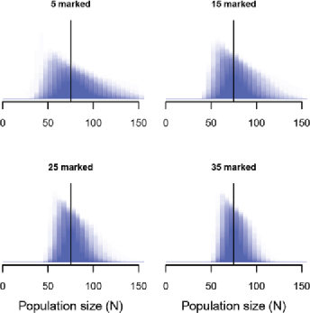
Figure 1: Simulation results demonstrating the effect of marking 5, 15, 25, and 35 individuals on the posterior distributions for population size. Each panel shows 200 overlaid posterior distributions, represented as histograms with transparent fill. The vertical line is the data generating value $N=75$.

Posterior distributions of $N$ for different numbers of marked individuals are shown in Figure 1. As anticipated, posterior precision increases substantially with the proportion of marked individuals. The posterior mode was approximately unbiased as a point estimator, and RMSE decreased 61% from 17.31 when all 75 individuals were unmarked to 6.82 when 35 individuals were marked (Tables 1 and 2). Coverage was close to nominal for all values of $m$ and posterior skew diminished as $m$ increased (Table 2).

=270pt # Marked Mean RMSE Mode RMSE Coverage $m=5$ 80.1 $14.53$ 75.9 $13.88$ 0.955 $m=15$ 78.4 $11.59$ 75.9 $11.26$ 0.945 $m=25$ 77.6 $8.51$ 75.7 $8.40$ 0.960 $m=35$ 77.0 $6.92$ 75.3 $6.82$ 0.960

Table 2: Posterior mean, mode, and 95% HPD interval coverage for simulations in which $m$ of $N=75$ individuals were marked. Two hundred simulations of each case were conducted

4.2 Point count data

We applied our model to point count data collected on the northern parula (Parula americana), a migratory passerine. This species maintains well-defined home ranges during the breeding season [Moldenhauer and Regelski (1996)], and thus our modeling effort was focused on estimating the number and location of home range centers. Points were located on a 50 m grid, which ensured spatial correlation since home ranges typically have $>$50 m radii and because their song can be heard from distance $>$50 m [Moldenhauer and Regelski (1996)]. This small grid spacing contrasts with the conventional practice of spacing points by $>$200 m to obtain i.i.d. counts. Figure 2 depicts the spatially correlated counts ($n_{r\cdot}$) from the 105 point count locations surveyed three times each during June 2006 at the Patuxent Wildlife Research Center in Laurel Maryland, USA. A total of 226 detections were made with a maximum count of 4 during a single survey. At 38 points, no Parulas were detected. All but one of the detections were of singing males, and this one observation was not included in the analysis.

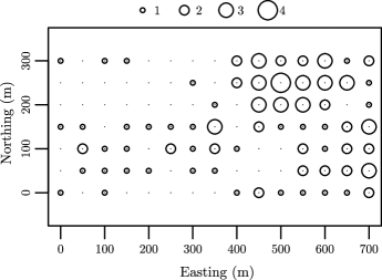
Figure 2: Spatially correlated counts of northern parula on a 50 m grid. The size of the circle represents the total number of detections at each point.

In our analysis of the Parula data, we defined the point process state-space by buffering the grid of point count locations by 250 m and used $M=300$ for data augmentation. We simulated posterior distributions using three Markov chains, each consisting of 300,000 iterations after discarding the initial 10,000 draws. Convergence was indicated by visual inspections of the Markov chain histories, and by $\hat{R}$ statistics [Gelman and Rubin (1992)] $<$1.1 for each of the monitored parameters: $\lambda_{0}$, $\sigma$, and $N$. The history plots are available in the supplementary material [Chandler and Royle (2013)].

Table 3: Posterior summary statistics for the spatial model applied to the northern parula data. Two sets of priors for the encounter rate parameter $\sigma$ were considered. $M=300$ was used in both cases. Parulas/ha, $D$, is a derived parameter

Par	Prior	Mean	SD	Mode	q0.025	q0.50	q0.975
$\sigma$	$U(0,\infty)$	$2.15$	$1.22$	$1.23$	$0.90$	$1.67$	$5.17$
$\lambda_{0}$	$U(0,\infty)$	$0.28$	$0.15$	$0.21$	$0.08$	$0.26$	$0.67$
$N$	$U(0,M)$	$40.95$	$38.07$	$4.00$	$3.00$	$31.00$	$143.00$
$D$	–	$0.43$	$0.40$	$0.04$	$0.031$	$0.32$	$1.49$
$\sigma$	$G(13,10)$	$1.30$	$0.26$	$1.23$	$0.90$	$1.27$	$1.91$
$\lambda_{0}$	$U(0,\infty)$	$0.30$	$0.13$	$0.24$	$0.10$	$0.28$	$0.60$
$N$	$U(0,M)$	$59.32$	$36.49$	$36.00$	$18.00$	$50.00$	$157.00$
$D$	–	$0.62$	$0.38$	$0.38$	$0.19$	$0.52$	$1.64$

One benefit of a Bayesian analysis is that it can accommodate prior information about home range size, which is readily available for many species and directly related to the encounter rate parameter $\sigma$ [Royle, Kéry and Guélat (2011)]. To illustrate, we analyzed the Parula data using two sets of priors. In the first set, all priors were improper, customary noninformative priors (see Table 3). Uniform priors were also used in the second set, with the exception of an informative prior for the scale parameter $\sigma\sim\operatorname{Gamma}(13,10)$. We arrived at this prior using the methods described by Royle, Kéry and Guélat (2011) and published information on home range size and detection probability [Moldenhauer and Regelski (1996), Simons et al. (2009)]. More details on this derivation are found in the supplementary material [Chandler and Royle (2013)]. We briefly note here that this prior includes the biologically plausible range of values for $\sigma$ suggested by the published literature.

The posterior distribution for $N$ was highly skewed with a long right tail resulting in a wide 95% credible interval (Table 3). Nonetheless, the interval for density, $D$, includes estimates reported from more intensive field studies [Moldenhauer and Regelski (1996)]. This was true when considering both sets of priors, although posterior precision was higher under the informative set of priors. Specifically, the use of prior information reduced posterior density at high, biologically implausible, values of $\sigma$, and hence decreased the posterior mass for low values of $N$ (Figure 3). For both sets of priors, $\operatorname{Pr}(N=M=300)\approx 0$, indicating that the amount of data augmentation was sufficient to avoid any effect on the posteriors.

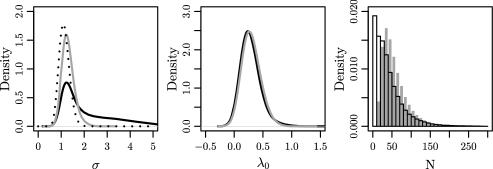
Figure 3: Effects of $\sigma\sim\operatorname{Gamma}(13,10)$ prior on the posterior distributions from the northern parula model. Posteriors from the model with uniform priors are shown in black, and posteriors from the informative prior model are shown in gray. The prior itself is shown as a dotted line in the leftmost panel.

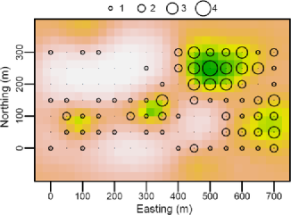
Figure 4: Estimated density surface of northern parula activity centers. The grid of point count locations with count totals is superimposed. See Figure 1 for additional details.

In addition to estimating density, our model can be used to produce density surface maps, which are often used in applied ecological research to direct management efforts and develop hypotheses regarding the factors influencing abundance. Density surface maps can be produced by discretizing the state-space and tallying the number of activity centers occurring in each pixel during each MCMC iteration. Parula density was highest near the northeastern corner of the study plot, which may correspond to important habitat features such as suitable nest site locations (Figure 4). We anticipate future model extensions to directly model the point process intensity using habitat covariates.

5 Discussion

In this paper we confronted one of the most difficult challenges faced in wildlife sampling—estimation of population density in the absence of data to distinguish among individuals. To do so, we developed a novel class of spatially explicit models that applies to spatially organized counts, where the count locations or traps are located sufficiently close together so that individuals are exposed to encounter at multiple traps. This design yields correlation in the observed counts, and this correlation proves to be informative about encounter rate parameters and density. We note that sample locations in count based studies are typically not organized close together in space because conventional wisdom and standard practice dictate that independence of sample units is necessary [Hurlbert (1984)]. Our model suggests that in some cases it might be advantageous to deviate from the conventional wisdom if one is interested in inference about density. Of course, this is also known in the application of standard spatial capture–recapture models [Borchers and Efford (2008)] where individual identity is preserved across trap encounters, but it is seldom, if ever, considered in the design of more traditional count surveys.

Our model has broad relevance to a vast number of animal sampling problems. The motivating problem involved bird point counts where individual identity is typically not available. The model also applies to other standard methods used to sample unmarked populations, such as camera traps or even methods that yield sign (e.g., scat, track) counts indexed by space. However, results of our simulation study reveal some important limitations of the basic estimator applied to situations in which none of the individuals can be uniquely identified. In particular, posterior distributions are highly skewed in typical small to moderate sample size situations and posterior precision is low, although for more expansive trapping grids, better performance can be expected.

Several modifications of the model can lead to improved performance of the estimator. Our simulation results demonstrate that marking a subset of individuals can yield substantial increases in posterior precision. Marking a subset of individuals is commonplace in animal studies such as when a small number of individuals are radio-collared in conjunction with a count based survey [Bartmann et al. (1987)]. In many other situations a subset of individuals can be identified by natural marks alone [Kelly et al. (2008)] and, thus, our model could be applied to data from camera trapping studies of species such as mountain lions, deer, or coyotes. The ability to study partially marked populations adds flexibility to existing SCR methods and also creates new opportunities for designing efficient SCR studies since the costs of marking all individuals in a population can be prohibitive.

When including data from marked individuals, it is important to note that we assume that the marks can be reliably read in the field, that is, there is no misidentification of marked animals. If some marked individuals cannot be reliably recognized, perhaps due to blurry photographs in camera trapping studies or DNA samples that do not amplify, then the questionable data records should be discarded so as not to bias estimators. Explicitly modeling misidentification of marked individuals deserves additional study.

When applied to data from marked and unmarked individuals, our model can be viewed as a spatial extension of traditional “mark-resight” estimators [Bartmann et al. (1987), Minta and Mangel (1989), McClintock and Hoeting (2010)]. In their simplest form, mark-resight methods involve fitting standard closed population capture–recapture models to the data on marked individuals, and the resultant estimate of detection probability ($\hat{p}$) is used to estimate population size as $\hat{N}=m+u/\hat{p}$, where $m$ and $u$ are the number of marked and unmarked individuals, respectively. In addition to the problem of converting $N$ to density, the unmarked individuals provide no information about the encounter rate parameters, and thus mark-resight methods cannot be used unless a large sample of marked individuals is available. This contrasts with our approach which can be used even when all individuals are unmarked.

In some cases, such as in point counts of birds, it may not be practical to mark individuals. An alternative to increasing posterior precision is to utilize prior information on home range size. Indeed, extensive information on home range size has been compiled for many species in diverse habitats [e.g., DeGraaf and Yamasaki (2001)]. It is easy to embody this information in a prior distribution as we demonstrated for the Parula data.

An additional design extension that could increase precision is to use multiple sampling methods [Gopalaswamy et al. (2012)], in which one method generates encounter frequencies and the other method generates individuality. For example, camera traps are now commonly used with surveys for sign (scat or tracks) or hair snares for sampling bear populations. These distinct methods would have different basal detection rates but share an underlying spatial model describing the organization of individuals in space. Our model shows promise for using these disparate data types efficiently for estimating density.

5.1 $N$-mixture models

Parallel developments which appear ostensibly unrelated to SCR models have addressed the problem of estimating population size when individuals are unmarked. $N$-mixture models [Royle (2004a, 2004b), Royle, Dawson and Bates (2004)] can be applied to a repeated measures type of data structure wherein data are collected at $J$ sites, with $K$ replicate surveys conducted at each. $N$-mixture models regard abundance at each site ($N_{j}$) as an i.i.d. realization from a discrete distribution, such as the Poisson or negative binomial with expectation $\theta$. In the standard binomial $N$-mixture model, the observed counts are treated as binomial outcomes with $N_{j}$ “trials” and detection probability $p$.

Although these models have proven useful for studies of factors that affect variation in abundance, interpretation of model parameters is strongly dependent on the assumption that populations are closed with respect to demographic processes and movement. The closure assumption can be an important practical limitation [but see Dail and Madsen (2011), Chandler, Royle and King (2011)]. Furthermore, the i.i.d. assumption is violated if spatial correlation exists among sites, such as if animals move among plots. Although we formulated the model developed in our paper as an extension of SCR models, it clearly can also be viewed as a spatially explicit extension of $N$-mixture models where the local population sizes $N_{j}$ are dependent owing to the nature of the sampling design.

Thus, two recently developed methodological frameworks, spatial capture–recapture and $N$-mixture models, address different problems that arise in sampling animal populations. SCR models address nonclosure by accommodating information on the juxtaposition of animal activity centers and traps, and $N$-mixture models address the inability to uniquely identify individuals. Our model unifies these two modeling frameworks by addressing both issues simultaneously.

5.2 Alternative observation models

Several aspects of our model can be modified to accommodate alternative sampling designs or parametric distributions. We considered situations in which an individual can be detected more than once at a trap during a single occasion, but under some designs this is not possible. When collecting DNA samples, for instance, an individual can often be detected at most once during an occasion, because multiple samples of biological material cannot be attributed to distinct episodes. Therefore, rather than $z_{ijk}\sim\operatorname{Pois}(\lambda_{ij})$, we have $z_{ijk}\sim\operatorname{Bern}(p_{ij})$ where, for example, $p_{ij}=p_{0}\exp(-d_{ij}^{2}/(2\sigma^{2}))$, and $p_{0}$ is the probability of detecting an individual whose home range is centered on trap $j$. This Bernoulli model is a focus of ongoing investigations.

Both the Poisson and the Bernoulli models produce count observations that when aggregated over individuals form trap-specific totals; however, ecologists often collect “detection/nondetection” data because it can be easier to determine if $\geq$1 individual was present rather than enumerating all individuals in a location. In this case, the underlying $z_{ijk}$ array is the same as the above cases, but we observe $n_{jk}=I(\sum_{i=1}^{N}z_{ijk}>0)$ where $I$ is the indicator function. This model is a spatially explicit extension of the model of Royle and Nichols (2003) in which the underlying abundance state is inferred from binary data. We have investigated this model to a limited extent but do not report on those results here.

5.3 Spatial point process models

Our model has some direct linkages to existing point process models. We note that the observation intensity function (i.e., corresponding to the observation locations) is a compound Gaussian kernel similar to that of the Thomas process [Møller and Waagepetersen (2003), pages 61 and 62, Thomas (1949)]. Also, the Poisson-Gamma convolution models [Wolpert and Ickstadt (1998)] are structurally similar [see also Higdon (1998) and Best, Ickstadt and Wolpert (2000)]. In particular, our model is such a model but with a constant basal encounter rate $\lambda_{0}$ and unknown number and location of “support points,” which in our case are the animal activity centers, $\{\mathbf{s}_{i}\}$. We can thus regard our model as an approach for estimating the location and local density of support points, which we believe could be useful in the application of convolution models. Best, Ickstadt and Wolpert (2000) devise an MCMC algorithm for the Poisson-Gamma model based on data augmentation, which is similar to the component of our algorithm for updating the missing data in the conditional-on-$\mathbf{z}$ formulation of the model. We emphasize that our model is distinct from these Poisson-Gamma models in that we estimate the number and location of such support points.

If individuals were perfectly observable, then the resulting point process of locations is clearly a standard Poisson or binomial (fixed $N$) cluster process or Neyman–Scott process. If detection is uniform over space but imperfect, then the basic process is unaffected by this random thinning. Our model can therefore be viewed formally as a Poisson (or binomial) cluster process model, but one in which the thinning is nonuniform, governed by the encounter model which dictates that the thinning rate increases with distance from the observation points. In addition, our inference objective is, essentially, to estimate the number of parents in the underlying Poisson cluster process, where the observations are biased by an incomplete sampling apparatus (points in space).

As a model of a thinned point process, our model has much in common with classical distance sampling models [Buckland et al. (2001), Johnson, Laake and Ver Hoef (2010)]. The main distinction is that our data structure does not include observed distances, although the underlying observation model is fundamentally the same as in distance sampling if there is only a single replicate sample and $\mathbf{s}_{i}$ is defined as an individual’s location at an instant in time. For replicate samples, our model preserves (latent) individuality across samples and traps which is not a feature of distance sampling. We note that error in measurement of distance is not a relevant consideration in our model, and we do not require the standard distance sampling assumption that the probability of detection is 1 if an individual occurs at the survey point. More importantly, distance sampling models cannot be applied to data from many of the sampling designs for which our model is relevant. For example, many rare and endangered species can only be effectively surveyed using noninvasive methods such as hair snares and camera traps that do not produce distance data [O’Connell, Nichols and Karanth (2011)].

6 Conclusion

Concerns about statistical independence have prompted ecologists to design count based studies such that the observed random variables can be regarded as i.i.d. outcomes [Hurlbert (1984)]. Interestingly, this often proves impossible in practice, and elaborate methods have been devised to model spatial dependence as a nuisance parameter. Conversely, our view is that spatial dependence is an important element of the underlying ecological process which is of direct interest in ecological investigations. Our paper presents a modeling framework that directly confronts the classical view of spatial dependence as a nuisance by demonstrating that spatial correlation carries information about the locations of individuals, which can be used to estimate density even when individuals are unmarked and distance-related heterogeneity exists in encounter probability.

References

- Bartmann et al. (1987) {barticle}[author] \bauthor\bsnmBartmann, \bfnmRichard M.\binitsR. M., \bauthor\bsnmWhite, \bfnmGary C.\binitsG. C., \bauthor\bsnmCarpenter, \bfnmLen H.\binitsL. H. and \bauthor\bsnmGarrott, \bfnmRobert A.\binitsR. A. (\byear1987). \btitleAerial mark-recapture estimates of confined mule deer in pinyon-juniper woodland. \bjournalThe Journal of Wildlife Management \bvolume51 \bpages41–46. \bptokimsref \endbibitem
- Best, Ickstadt and Wolpert (2000) {barticle}[mr] \bauthor\bsnmBest, \bfnmNicola G.\binitsN. G., \bauthor\bsnmIckstadt, \bfnmKatja\binitsK. and \bauthor\bsnmWolpert, \bfnmRobert L.\binitsR. L. (\byear2000). \btitleSpatial Poisson regression for health and exposure data measured at disparate resolutions. \bjournalJ. Amer. Statist. Assoc. \bvolume95 \bpages1076–1088. \biddoi=10.2307/2669744, issn=0162-1459, mr=1821716 \bptokimsref \endbibitem
- Borchers and Efford (2008) {barticle}[mr] \bauthor\bsnmBorchers, \bfnmD. L.\binitsD. L. and \bauthor\bsnmEfford, \bfnmM. G.\binitsM. G. (\byear2008). \btitleSpatially explicit maximum likelihood methods for capture–recapture studies. \bjournalBiometrics \bvolume64 \bpages377–385, 664. \biddoi=10.1111/j.1541-0420.2007.00927.x, issn=0006-341X, mr=2432407 \bptokimsref \endbibitem
- Buckland et al. (2001) {bbook}[author] \bauthor\bsnmBuckland, \bfnmS. T\binitsS. T., \bauthor\bsnmAnderson, \bfnmD. R.\binitsD. R., \bauthor\bsnmBurnham, \bfnmK. P.\binitsK. P., \bauthor\bsnmLaake, \bfnmJ. L.\binitsJ. L., \bauthor\bsnmBorchers, \bfnmD. L.\binitsD. L. and \bauthor\bsnmThomas, \bfnmL.\binitsL. (\byear2001). \btitleIntroduction to Distance Sampling: Estimating Abundance of Biological Populations. \bpublisherOxford Univ. Press, \blocationOxford. \bptokimsref \endbibitem
- Chandler, Royle and King (2011) {barticle}[pbm] \bauthor\bsnmChandler, \bfnmRichard B.\binitsR. B., \bauthor\bsnmRoyle, \bfnmJ. Andrew\binitsJ. A. and \bauthor\bsnmKing, \bfnmDavid I.\binitsD. I. (\byear2011). \btitleInference about density and temporary emigration in unmarked populations. \bjournalEcology \bvolume92 \bpages1429–1435. \bidissn=0012-9658, pmid=21870617 \bptokimsref \endbibitem
- Chandler and Royle (2013) {bmisc}[author] \bauthor\bsnmChandler, \bfnmRichard B.\binitsR. B. and \bauthor\bsnmRoyle, \bfnmJ. Andrew\binitsJ. A. (\byear2013). \bhowpublishedSupplement to “Spatially explicit models for inference about density in unmarked or partially marked populations.” DOI:\doiurl10.1214/12-AOAS610SUPP. \bptokimsref \endbibitem
- Dail and Madsen (2011) {barticle}[mr] \bauthor\bsnmDail, \bfnmD.\binitsD. and \bauthor\bsnmMadsen, \bfnmL.\binitsL. (\byear2011). \btitleModels for estimating abundance from repeated counts of an open metapopulation. \bjournalBiometrics \bvolume67 \bpages577–587. \biddoi=10.1111/j.1541-0420.2010.01465.x, issn=0006-341X, mr=2829026 \bptokimsref \endbibitem
- Dawson and Efford (2009) {barticle}[author] \bauthor\bsnmDawson, \bfnmD. K.\binitsD. K. and \bauthor\bsnmEfford, \bfnmM. G.\binitsM. G. (\byear2009). \btitleBird population density estimated from acoustic signals. \bjournalJournal of Applied Ecology \bvolume46 \bpages1201–1209. \bptokimsref \endbibitem
- DeGraaf and Yamasaki (2001) {bbook}[author] \bauthor\bsnmDeGraaf, \bfnmR. M\binitsR. M. and \bauthor\bsnmYamasaki, \bfnmM.\binitsM. (\byear2001). \btitleNew England Wildlife: Habitat, Natural History, and Distribution. \bpublisherUniv. Press of New England, \blocationHanover, NH. \bptokimsref \endbibitem
- Dice (1938) {barticle}[author] \bauthor\bsnmDice, \bfnmL. R.\binitsL. R. (\byear1938). \btitleSome census methods for mammals. \bjournalThe Journal of Wildlife Management \bvolume2 \bpages119–130. \bptokimsref \endbibitem
- Efford (2004) {barticle}[author] \bauthor\bsnmEfford, \bfnmMurray\binitsM. (\byear2004). \btitleDensity estimation in live-trapping studies. \bjournalOikos \bvolume106 \bpages598–610. \bptokimsref \endbibitem
- Efford, Dawson and Borchers (2009) {barticle}[pbm] \bauthor\bsnmEfford, \bfnmMurray G.\binitsM. G., \bauthor\bsnmDawson, \bfnmDeanna K.\binitsD. K. and \bauthor\bsnmBorchers, \bfnmDavid L.\binitsD. L. (\byear2009). \btitlePopulation density estimated from locations of individuals on a passive detector array. \bjournalEcology \bvolume90 \bpages2676–2682. \bidissn=0012-9658, pmid=19886477 \bptokimsref \endbibitem
- Gardner, Royle and Wegan (2009) {barticle}[pbm] \bauthor\bsnmGardner, \bfnmBeth\binitsB., \bauthor\bsnmRoyle, \bfnmJ. Andrew\binitsJ. A. and \bauthor\bsnmWegan, \bfnmMichael T.\binitsM. T. (\byear2009). \btitleHierarchical models for estimating density from DNA mark-recapture studies. \bjournalEcology \bvolume90 \bpages1106–1115. \bidissn=0012-9658, pmid=19449704 \bptokimsref \endbibitem
- Gelman and Rubin (1992) {barticle}[author] \bauthor\bsnmGelman, \bfnmA.\binitsA. and \bauthor\bsnmRubin, \bfnmD. B.\binitsD. B. (\byear1992). \btitleInference from iterative simulation using multiple sequences. \bjournalStatist. Sci. \bvolume7 \bpages457–511. \bptokimsref \endbibitem
- Gopalaswamy et al. (2012) {barticle}[pbm] \bauthor\bsnmGopalaswamy, \bfnmArjun M.\binitsA. M., \bauthor\bsnmRoyle, \bfnmJ. Andrew\binitsJ. A., \bauthor\bsnmDelampady, \bfnmMohan\binitsM., \bauthor\bsnmNichols, \bfnmJames D.\binitsJ. D., \bauthor\bsnmKaranth, \bfnmK. Ullas\binitsK. U. and \bauthor\bsnmMacdonald, \bfnmDavid W.\binitsD. W. (\byear2012). \btitleDensity estimation in tiger populations: Combining information for strong inference. \bjournalEcology \bvolume93 \bpages1741–1751. \bidissn=0012-9658, pmid=22919919 \bptokimsref \endbibitem
- Higdon (1998) {barticle}[author] \bauthor\bsnmHigdon, \bfnmD.\binitsD. (\byear1998). \btitleA process-convolution approach to modelling temperatures in the North Atlantic Ocean. \bjournalEnviron. Ecol. Stat. \bvolume5 \bpages173–190. \bptokimsref \endbibitem
- Higdon (2002) {bincollection}[mr] \bauthor\bsnmHigdon, \bfnmDave\binitsD. (\byear2002). \btitleSpace and space–time modeling using process convolutions. In \bbooktitleQuantitative Methods for Current Environmental Issues (\beditorC. W. Anderson, \beditorV. Barnett, \beditorP. C. Chatwin and \beditorA. H. El-Shaarawi, eds.) \bpages37–56. \bpublisherSpringer, \blocationLondon. \bidmr=2059819 \bptokimsref \endbibitem
- Hurlbert (1984) {barticle}[author] \bauthor\bsnmHurlbert, \bfnmS. H.\binitsS. H. (\byear1984). \btitlePseudoreplication and the design of ecological field experiments. \bjournalEcological Monographs \bvolume54 \bpages187–211. \bptokimsref \endbibitem
- Illian et al. (2008) {bbook}[mr] \bauthor\bsnmIllian, \bfnmJanine\binitsJ., \bauthor\bsnmPenttinen, \bfnmAntti\binitsA., \bauthor\bsnmStoyan, \bfnmHelga\binitsH. and \bauthor\bsnmStoyan, \bfnmDietrich\binitsD. (\byear2008). \btitleStatistical Analysis and Modelling of Spatial Point Patterns. \bpublisherWiley, \blocationChichester. \bidmr=2384630 \bptokimsref \endbibitem
- Johnson, Laake and Ver Hoef (2010) {barticle}[mr] \bauthor\bsnmJohnson, \bfnmDevin S.\binitsD. S., \bauthor\bsnmLaake, \bfnmJeffrey L.\binitsJ. L. and \bauthor\bsnmVer Hoef, \bfnmJay M.\binitsJ. M. (\byear2010). \btitleA model-based approach for making ecological inference from distance sampling data. \bjournalBiometrics \bvolume66 \bpages310–318. \biddoi=10.1111/j.1541-0420.2009.01265.x, issn=0006-341X, mr=2756719 \bptnotecheck year\bptokimsref \endbibitem
- Kelly et al. (2008) {barticle}[author] \bauthor\bsnmKelly, \bfnmM. J.\binitsM. J., \bauthor\bsnmNoss, \bfnmA. J.\binitsA. J., \bauthor\bsnmDi Bitetti, \bfnmM. S.\binitsM. S., \bauthor\bsnmMaffei, \bfnmL.\binitsL., \bauthor\bsnmArispe, \bfnmR. L.\binitsR. L., \bauthor\bsnmPaviolo, \bfnmA.\binitsA., \bauthor\bsnmDe Angelo, \bfnmC. D.\binitsC. D. and \bauthor\bsnmDi Blanco, \bfnmY. E.\binitsY. E. (\byear2008). \btitleEstimating puma densities from camera trapping across three study sites: Bolivia, Argentina, and Belize. \bjournalJournal of Mammalogy \bvolume89 \bpages408–418. \bptokimsref \endbibitem
- Liu and Wu (1999) {barticle}[mr] \bauthor\bsnmLiu, \bfnmJun S.\binitsJ. S. and \bauthor\bsnmWu, \bfnmYing Nian\binitsY. N. (\byear1999). \btitleParameter expansion for data augmentation. \bjournalJ. Amer. Statist. Assoc. \bvolume94 \bpages1264–1274. \bidissn=0162-1459, mr=1731488 \bptokimsref \endbibitem
- McClintock and Hoeting (2010) {barticle}[mr] \bauthor\bsnmMcClintock, \bfnmBrett T.\binitsB. T. and \bauthor\bsnmHoeting, \bfnmJennifer A.\binitsJ. A. (\byear2010). \btitleBayesian analysis of abundance for binomial sighting data with unknown number of marked individuals. \bjournalEnviron. Ecol. Stat. \bvolume17 \bpages317–332. \biddoi=10.1007/s10651-009-0109-0, issn=1352-8505, mr=2725770 \bptnotecheck year\bptokimsref \endbibitem
- Minta and Mangel (1989) {barticle}[author] \bauthor\bsnmMinta, \bfnmSteven\binitsS. and \bauthor\bsnmMangel, \bfnmMarc\binitsM. (\byear1989). \btitleA simple population estimate based on simulation for capture–recapture and capture-resight data. \bjournalEcology \bvolume70 \bpages1738–1751. \bptokimsref \endbibitem
- Moldenhauer and Regelski (1996) {bincollection}[author] \bauthor\bsnmMoldenhauer, \bfnmRalph R.\binitsR. R. and \bauthor\bsnmRegelski, \bfnmDaniel J.\binitsD. J. (\byear1996). \btitleNorthern Parula (Parula americana). In \bbooktitleThe Birds of North America Online (\beditor\bfnmA.\binitsA. \bsnmPoole, ed.). \bpublisherCornell Lab of Ornithology, \blocationIthaca, NY. \bptokimsref \endbibitem
- Møller and Waagepetersen (2003) {bbook}[author] \bauthor\bsnmMøller, \bfnmJ.\binitsJ. and \bauthor\bsnmWaagepetersen, \bfnmR. P.\binitsR. P. (\byear2003). \btitleStatistical Inference and Simulation for Spatial Point Processes. \bpublisherCRC Press, \blocationBoca Raton, FL. \bptokimsref \endbibitem
- O’Connell, Nichols and Karanth (2011) {bbook}[author] \bauthor\bsnmO’Connell, \bfnmA. F.\binitsA. F., \bauthor\bsnmNichols, \bfnmJ. D.\binitsJ. D. and \bauthor\bsnmKaranth, \bfnmU. K.\binitsU. K. (\byear2011). \btitleCamera Traps in Animal Ecology: Methods and Analyses. \bpublisherSpringer, \blocationNew York. \bptokimsref \endbibitem
- Royle (2004a) {barticle}[mr] \bauthor\bsnmRoyle, \bfnmJ. Andrew\binitsJ. A. (\byear2004a). \btitle-mixture models for estimating population size from spatially replicated counts. \bjournalBiometrics \bvolume60 \bpages108–115. \biddoi=10.1111/j.0006-341X.2004.00142.x, issn=0006-341X, mr=2043625 \bptokimsref \endbibitem
- Royle (2004b) {barticle}[author] \bauthor\bsnmRoyle, \bfnmJ. A.\binitsJ. A. (\byear2004b). \btitleGeneralized estimators of avian abundance from count survey data. \bjournalAnimal Biodiversity and Conservation \bvolume27 \bpages375–386. \bptokimsref \endbibitem
- Royle, Dawson and Bates (2004) {barticle}[author] \bauthor\bsnmRoyle, \bfnmJ. A.\binitsJ. A., \bauthor\bsnmDawson, \bfnmD. K.\binitsD. K. and \bauthor\bsnmBates, \bfnmS.\binitsS. (\byear2004). \btitleModeling abundance effects in distance sampling. \bjournalEcology \bvolume85 \bpages1591–1597. \bptokimsref \endbibitem
- Royle, Dorazio and Link (2007) {barticle}[mr] \bauthor\bsnmRoyle, \bfnmJ. Andrew\binitsJ. A., \bauthor\bsnmDorazio, \bfnmRobert M.\binitsR. M. and \bauthor\bsnmLink, \bfnmWilliam A.\binitsW. A. (\byear2007). \btitleAnalysis of multinomial models with unknown index using data augmentation. \bjournalJ. Comput. Graph. Statist. \bvolume16 \bpages67–85. \biddoi=10.1198/106186007X181425, issn=1061-8600, mr=2345748 \bptokimsref \endbibitem
- Royle and Dorazio (2012) {barticle}[author] \bauthor\bsnmRoyle, \bfnmJ. A.\binitsJ. A. and \bauthor\bsnmDorazio, \bfnmR. M.\binitsR. M. (\byear2012). \btitleParameter-expanded data augmentation for Bayesian analysis of capture–recapture models. \bjournalJournal of Ornithology \bvolume152 \bpagesS521–S537. \bptokimsref \endbibitem
- Royle, Kéry and Guélat (2011) {barticle}[author] \bauthor\bsnmRoyle, \bfnmJ. A.\binitsJ. A., \bauthor\bsnmKéry, \bfnmM.\binitsM. and \bauthor\bsnmGuélat, \bfnmJ.\binitsJ. (\byear2011). \btitleSpatial capture–recapture models for search-encounter data. \bjournalMethods in Ecology and Evolution \bvolume2 \bpages602–611. \bptokimsref \endbibitem
- Royle and Nichols (2003) {barticle}[author] \bauthor\bsnmRoyle, \bfnmJ. Andrew\binitsJ. A. and \bauthor\bsnmNichols, \bfnmJames D.\binitsJ. D. (\byear2003). \btitleEstimating abundance from repeated presence-absence data or point counts. \bjournalEcology \bvolume84 \bpages777–790. \bptokimsref \endbibitem
- Royle and Young (2008) {barticle}[author] \bauthor\bsnmRoyle, \bfnmJ. Andrew\binitsJ. A. and \bauthor\bsnmYoung, \bfnmKevin V.\binitsK. V. (\byear2008). \btitleA hierarchical model for spatial capture–recapture data. \bjournalEcology \bvolume89 \bpages2281–2289. \bptokimsref \endbibitem
- Royle et al. (2009) {barticle}[pbm] \bauthor\bsnmRoyle, \bfnmJ. Andrew\binitsJ. A., \bauthor\bsnmKaranth, \bfnmK. Ullas\binitsK. U., \bauthor\bsnmGopalaswamy, \bfnmArjun M.\binitsA. M. and \bauthor\bsnmKumar, \bfnmN. Samba\binitsN. S. (\byear2009). \btitleBayesian inference in camera trapping studies for a class of spatial capture–recapture models. \bjournalEcology \bvolume90 \bpages3233–3244. \bidissn=0012-9658, pmid=19967878 \bptokimsref \endbibitem
- Seber (1973) {bbook}[author] \bauthor\bsnmSeber, \bfnmG. A. F.\binitsG. A. F. (\byear1973). \btitleThe Estimation of Animal Abundance and Related Parameters. \bpublisherGriffin, \blocationLondon. \bptokimsref \endbibitem
- Simons et al. (2009) {bincollection}[author] \bauthor\bsnmSimons, \bfnmTheodore R.\binitsT. R., \bauthor\bsnmPollock, \bfnmKenneth H.\binitsK. H., \bauthor\bsnmWettroth, \bfnmJohn M.\binitsJ. M., \bauthor\bsnmAlldredge, \bfnmMathew W.\binitsM. W., \bauthor\bsnmPacifici, \bfnmKrishna\binitsK. and \bauthor\bsnmBrewster, \bfnmJerome\binitsJ. (\byear2009). \btitleSources of measurement error, misclassification error, and bias in auditory avian point count data. In \bbooktitleModeling Demographic Processes In Marked Populations 3 (\beditor\bfnmDavid L\binitsD. L. \bsnmThomson, \beditor\bfnmEvan G.\binitsE. G. \bsnmCooch and \beditor\bfnmMichael J.\binitsM. J. \bsnmConroy, eds.) \bpages237–254. \bpublisherSpringer, \blocationBoston, MA. \bptokimsref \endbibitem
- Sollmann et al. (2011) {barticle}[author] \bauthor\bsnmSollmann, \bfnmR.\binitsR., \bauthor\bsnmFurtado, \bfnmM. M.\binitsM. M., \bauthor\bsnmGardner, \bfnmB.\binitsB., \bauthor\bsnmHofer, \bfnmH.\binitsH., \bauthor\bsnmJácomo, \bfnmA. T. A.\binitsA. T. A., \bauthor\bsnmTôrres, \bfnmN. M.\binitsN. M. and \bauthor\bsnmSilveira, \bfnmL.\binitsL. (\byear2011). \btitleImproving density estimates for elusive carnivores: Accounting for sex-specific detection and movements using spatial capture–recapture models for jaguars in central Brazil. \bjournalBiological Conservation \bvolume144 \bpages1017–1024. \bptokimsref \endbibitem
- Tanner and Wong (1987) {barticle}[mr] \bauthor\bsnmTanner, \bfnmMartin A.\binitsM. A. and \bauthor\bsnmWong, \bfnmWing Hung\binitsW. H. (\byear1987). \btitleThe calculation of posterior distributions by data augmentation. \bjournalJ. Amer. Statist. Assoc. \bvolume82 \bpages528–540. \bptokimsref \endbibitem
- Thomas (1949) {barticle}[mr] \bauthor\bsnmThomas, \bfnmMarjorie\binitsM. (\byear1949). \btitleA generalization of Poisson’s binomial limit for use in ecology. \bjournalBiometrika \bvolume36 \bpages18–25. \bidissn=0006-3444, mr=0033999 \bptokimsref \endbibitem
- Wilson and Anderson (1985) {barticle}[author] \bauthor\bsnmWilson, \bfnmKenneth R.\binitsK. R. and \bauthor\bsnmAnderson, \bfnmDavid R.\binitsD. R. (\byear1985). \btitleEvaluation of two density estimators of small mammal population size. \bjournalJournal of Mammalogy \bvolume66 \bpages13–21. \bptokimsref \endbibitem
- Wolpert and Ickstadt (1998) {barticle}[mr] \bauthor\bsnmWolpert, \bfnmRobert L.\binitsR. L. and \bauthor\bsnmIckstadt, \bfnmKatja\binitsK. (\byear1998). \btitlePoisson/gamma random field models for spatial statistics. \bjournalBiometrika \bvolume85 \bpages251–267. \biddoi=10.1093/biomet/85.2.251, issn=0006-3444, mr=1649114 \bptokimsref \endbibitem