Measuring every particle’s size from three-dimensional imaging experiments

Abstract

Often experimentalists study particulate samples that are nominally monodisperse. In reality many samples have a polydispersity of 4-10%. At the level of an individual particle, the consequences of this polydispersity are unknown as it is difficult to measure an individual particle size from images of a dense sample. We propose a method to estimate individual particle radii from three-dimensional data of the particle positions. We validate our method by numerical simulations of four major systems: random close packing, colloidal gels, nominally monodisperse dense samples, and nominally binary dense samples. We then apply our method to experimental data from moderately concentrated colloidal suspensions observed with confocal microscopy. We demonstrate that we can recover the full particle size distribution in situ. Lastly, we use our method to study the relationship between homogeneous colloidal crystal nucleation and particle sizes. We show that nucleation occurs in regions that are more monodisperse than average.

A wide variety of techniques exist for three-dimensional imaging of collections of particles dijksman12 ; prasad07 . These types of samples include granular materials, soil mechanics, and colloidal suspensions. Our particular interest is in colloidal suspensions; these have been successfully used as model systems for understanding phase transitions for several decades Pusey ; Lekkerkerker , and moreover are interesting in their own right due to industrial relevance Vincent . Confocal microscopy can be used to take three-dimensional images of fluorescent colloidal particles deep within a sample vanblaaderen92 ; Blaaderen1 ; prasad07 . When coupled with particle tracking techniques, the motion of thousands of individual colloidal particles can be followed over long periods of time kegel00 ; EricSci ; Eric2002 ; Dinsmore . This technique has been used to investigate the colloidal glass transition Blaaderen1 ; kegel00 ; EricSci ; Eric2002 ; Narumi , crystallization Blaaderen2 ; Gasser ; Dullens06 , colloidal gels dinsmore02gel ; dibble06 ; gao07 , capillary waves aarts04 ; hernandez09 , sedimentation Blaaderen2 ; Paddy , and a variety of other questions (see ref. prasad07 for a review). One advantage of confocal microscopy of colloids is that the data obtained are similar to what is found using simulations, which also provide the data of particle positions over long periods of time.

However, experimental samples are always polydisperse: even for a nominally single-component sample, the particles have a variety of sizes poon12 . This is quantified by the polydispersity $p$, defined as the standard deviation of particle radii divided by the mean radius. For many samples, $p\sim 0.04-0.10$ poon12 . From numerical simulations, we know that the effects of the particle size distribution are not negligible. For example, crystal nucleation is difficult or impossible for more polydisperse samples Frenkel ; pusey09 . The crystal-liquid phase boundary depends on the polydispersity sollich10 . The sensitivity to volume fraction near the glass transition depends on the composition in nontrivial ways KAT ; KW2 . Experimentally, the influence of polydispersity on colloidal crystallization has been demonstrated schope07 ; henderson98 , and there is also some understanding of how the particle size distribution influences the rheological behavior of a colloidal sample mewis94 . However, these are limited to studies of the spatially averaged properties of the sample. Microscopy is useful for local properties, but particle size fluctuations of $0.04-0.10$ are not easily detectable. It would be desirable to know particle sizes for more direct comparison with simulations. Furthermore, in some cases, neglecting these sizes in an experiment can lead to wrong conclusions. One example is that the pair correlation function $g(r)$ can show a qualitatively incorrect dependence on control parameters if the particle sizes are treated as all identical pond11 . A second example is that the apparent compressibility of a random close packed sample depends qualitatively on whether individual particle sizes are taken into account Berthier ; Zachary1 ; KW3 .

In this work, we introduce a general method for using 3D data to determine the size of individual particles in any moderately concentrated sample, in general with volume fractions $\phi\gtrsim 0.4$. We use simulation data to verify that our method works well in a variety of sample types. We then demonstrate the utility of our method using previously published experimental data from confocal microscopy of colloids. In particular, we show that colloidal crystal nucleation is sensitive to the local polydispersity: nucleation happens in locally monodisperse regions. Our method is not limited to confocal microscopy and colloidal samples, but rather works with any data of the 3D positions of a collection of particles.

Due to diffraction limits, it is difficult to directly determine the radii of individual particles from microscopy images to better than $\pm 0.1$ $\mu$m brujic03 . Defining the edge is somewhat arbitrary and varies depending on particle properties and the details of the microscope illumination. Other 3D imaging techniques have similar issues dijksman12 .

In contrast, it is much easier to calculate the mean radius $\bar{a}$ of particles with a variety of techniques poon12 . Likewise, from the centers of particles, the separations between neighboring particles $r_{ij}$ can be easily calculated. Our estimation method for particle sizes uses only $\bar{a}$ and $r_{ij}$. The key idea of our method is that a large particle will be slightly farther from its neighbors and thus have larger values for its $r_{ij}$, and likewise a smaller particle will have smaller values of $r_{ij}$.

To start, we relate the pairwise separations $r_{ij}$ as

$$r_{ij}(t)=a_{i}+a_{j}+\delta_{ij}(t),$$ (1)

where particle $j$ is a nearest neighbor particle of particle $i$, $r_{ij}$ is the measured distance between $i$ and $j$, $a_{i}$ and $a_{j}$ are their radii, and $\delta_{ij}(t)$ is a surface-to-surface distance between their particles. We typically consider $5-7$ nearest neighbor particles (the closest neighbors); this choice is justified below. Often these data come from particle tracking Dinsmore ; Crocker and so $r_{ij}(t)$ and $\delta_{ij}(t)$ depend on time $t$. Next we take an average of $r_{ij}$ with respect to the nearest neighbor particles $j$, and then $\langle r_{ij}(t)\rangle_{j}=a_{i}+\langle a_{j}\rangle_{j}+\langle\delta_{ij}(t)\rangle_{j}$, where $\langle\rangle_{j}$ means an average over particle $j$. Thus, we obtain

$$a_{i}=\langle r_{ij}(t)\rangle_{j}-\langle a_{j}\rangle_{j}-\langle\delta_{ij}(t)\rangle_{j}.$$ (2)

This is exact, but the quantities $\delta_{ij}(t)$ are unknown. We estimate this by replacing $\delta_{ij}(t)$ with its time- and particle-averaged value, the mean gap distance $\bar{\delta}\equiv\langle r_{ij}(t)\rangle_{i,j,t}-2\bar{a}$, where the average is over all particle pairs and all times. Our algorithm is then:

$$a_{i}^{(0)}(t) = \bar{a},$$ (3)

$$a_{i}^{(n)}(t) = \langle r_{ij}(t)\rangle_{j}-\langle a_{j}^{(n-1)}(t)\rangle_{j}-\bar{\delta},$$ (4)

where the superscripts denote iteration. The more we iterate Eq. 4, the more information we obtain from particles far away from a given particle. In fact, $a_{i}^{(n)}(t)$ is unchanged for $n\geq 10$ since $a_{i}^{(10)}$ includes the information from several thousand particles, thus we fix $n=10$ for the number of iterations in this paper. Of course, the particle radius does not depend on time, so after the 10th iteration, we time-average $a_{i}^{(10)}(t)$ to obtain the estimated particle radius $a_{i}^{(10)}$. Time-averaging after each iteration of Eq. 4 does not change the results.

There are several sources of uncertainty in this estimation. First, there is the uncertainty of each particle position. Typically this is about 5-8% of the mean radius, leading to a 8-10% uncertainty of $r_{ij}$ EricSci ; Dinsmore ; Crocker . However, these errors are nearly time-independent, so those errors are greatly diminished by time averaging. Second, our approximation for $\bar{\delta}$ is weaker in the case that the distribution of $\delta_{ij}(t)$ is broad. This in part depends on how many nearest neighbor particles are chosen: more neighbors results in a broader distribution, whereas too few neighbors means that the average $\langle r_{ij}(t)\rangle$ in Eq. 4 is poor. Below, we use simulation data to determine that $Z=5-7$ nearest neighbors is an optimal choice. Third, independent of a given choice of $Z$, some particles will simply be farther from their neighbors, and some will be closer. In a dense suspension, for example, this relates to the size of the “cage” formed by the nearest neighbor particles Eric2002 . Again, time averaging helps. If particles can rearrange and find new neighbors, then $\bar{\delta}$ becomes a better approximation for $\langle\delta_{ij}(t)\rangle_{t}$. In dense colloidal suspensions with volume fractions $\phi\gtrsim 0.5$, rearrangements become infrequent and so longer time averages are desired kegel00 ; EricSci ; Eric2002 . In summary, the greatest strength of our algorithm is time-averaging, and past that, a sensible choice for the number of nearest neighbors $Z$ is useful. Our tests show that time averaging over $\sim 20$ different times is sufficient for reasonable results.

To verify our radius estimation method, we simulate a variety of systems and compare the estimated radius of each particle with its true radius. The error is given by $\delta a_{i}=a_{i}^{(10)}-a_{i}$, where $a_{i}^{(10)}$ is the estimated value and $a_{i}$ is the true value. $\Delta a\equiv\langle\delta a_{i}\rangle/\bar{a}$ is the mean fractional error in the estimated particle radius. Also relevant is the polydispersity $p$ of the simulated sample, defined as $p=\sqrt{\langle(a_{i}-\bar{a})^{2}\rangle}/\bar{a}$, where the averages are over all particles $i$. Before any estimation is applied, the best guess for each particle size is $\bar{a}$ with a fractional uncertainty $p$. If the mean estimation error $\Delta a$ is less than $p$, the estimation method improves our knowledge of the particle sizes; we will show this is true for the simulated data.

Our first test case is a random close packed sample. In such a sample particles do not move, and so time-averaging cannot be used. However, particles are packed so that they contact each other, that is, $\bar{\delta}=0$. The number of contacting neighbors varies from particle to particle, so it is not clear how many neighbors should be considered. Accordingly, we plot $\Delta a$ as a function of $Z$ in Fig. 1A. We find that $\Delta a$ is a minimum at $Z$ = 5, and is indeed much smaller than $p$ (0.01 vs. 0.07 in this case).

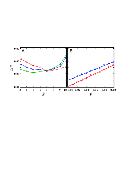
Figure 1: (Color online) Dependence of estimation uncertainty $\Delta a$ on parameters. (A) The uncertainty $\Delta a$ as a function of the chosen number of neighbors $Z$ used for the averaging. The circles, triangles and squares correspond to $\Delta a$ for volume fractions $\phi$ = 0.51, 0.56, and 0.64 (RCP), respectively. In each case, the sample polydispersity is $p=0.07$. (B) $\Delta a$ as a function of the bulk polydispersity $p$. The circles and the triangles correspond to $\Delta a$ at RCP and $\phi$ = 0.51, respectively. The solid lines are the fitting lines for $\Delta a$.

It is possible that while $\Delta a$ is small, that there are systematic errors depending on the real particle size $a_{i}$. To test this, in Fig. 2A we show the ratio between the estimated radius and the given radius $a_{i}^{(10)}/a_{i}$ as a function of $a_{i}$ for a polydispersity $p=0.07$ RCP sample. The symbols and the error bars correspond to the mean and standard deviation of the distribution of $a_{i}^{(10)}/a_{i}$ between [$a_{i},a_{i}+0.01$], respectively. $a_{i}^{(10)}/a_{i}$ should be 1 if our estimation is perfect and indeed we find $a_{i}^{(10)}/a_{i}=1.000\pm 0.013$. The quality of the results is nearly uniform as a function of particle size. To check the validity of our method for RCP samples with different polydispersity, we plot the uncertainty $\Delta a$ as a function of sample polydispersity $p$ in Fig. 1B. We find $\Delta a\approx p/6$ KW3 .

A colloidal gel shares a similarity to a RCP sample (touching particles), and has a significant difference (much lower volume fraction). In a colloidal gel particles are stuck to their neighbors and form a large network. Often the attractive interactions have a finite range, for example with depletion gels AO [see discussion in Methods]. Thus we note that the distribution of $\delta_{ij}$ for gels is slightly broader than that for RCP, though the mean average of $\delta_{ij}$ is close to 0. Some time averaging is possible, although such samples are frequently nonergodic or at best rearrange quite slowly.

Likewise the contacting particles make gels similar to RCP samples locally. However, the contact number fluctuates greatly in a colloidal gel, and the number of neighbors averaged over must vary from particle to particle. Rather than being a fixed parameter $Z$, we have a varying number of neighbors $Z_{i}$ used in the average (Eq. 4). To determine $Z_{i}$, we define the coordination number $c_{i}$ as the number of particles within a distance 2.8$a$, which is the first minimum of the pair correlation function. We find the average coordination number $\bar{c}\approx 13.1$ for a RCP sample, but this will generally be smaller for a gel dinsmore02gel . Thus for every particle we estimate the number of touching neighbors $Z_{i}=5c_{i}/13$ where we round $Z_{i}$ to the nearest integer. In general, given the tenuous nature of a gel, for many particles $Z_{i}$ is fairly small; also, $\delta_{ij}$ has a broader distribution, and so $\Delta a$ will be worse than the RCP case. However, $\Delta a$ is improved by time-averaging, which also minimizes the uncertainty due to particle tracking errors. Fig. 2B shows the ratio between the time-averaged estimated radius and the given radius $a_{i}^{(10)}/a_{i}$ as a function of the true radius $a_{i}$ for the colloidal gel. We find that $a_{i}^{(10)}/a_{i}=1.000\pm 0.018$. $\Delta a=0.018$ is much smaller than the polydispersity $p=0.07$.

Moving from gels, we next consider a dense suspension of purely repulsive (hard-sphere) particles. Here no particles are in contact, so $\delta_{ij}$ has a much broader distribution; however, time-averaging is even more powerful. We show $a_{i}^{(10)}/a_{i}$ as a function of $a_{i}$ at $\phi=0.51$ in Fig. 2C, finding $a_{i}^{(10)}/a_{i}=1.000\pm 0.014$. Yet again $\Delta a=0.014$ is much smaller than the polydispersity $p=0.070$.

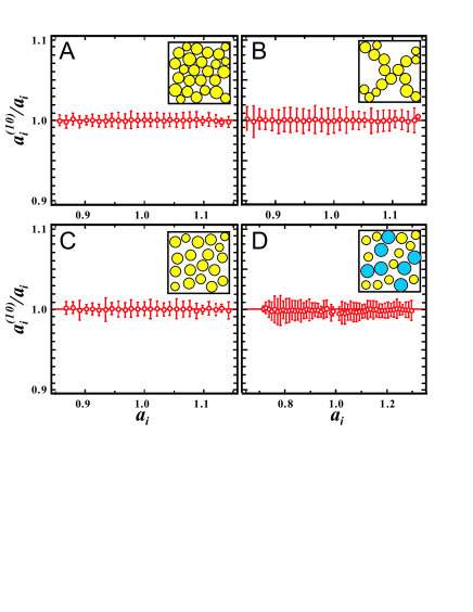
Figure 2: (Color online) The estimated radius $a_{i}^{(10)}/a_{i}$ as a function of the true radius $a_{i}$, for four simulated systems: (A) random close packing, (B) a colloidal gel at $\phi=0.10$, (C) a nominally monodisperse suspension at $\phi=0.51$, and (D) a nominally binary suspension at $\phi=0.51$. For (A-C), the polydispersities are $p=0.07$. For the binary sample, the size ratio is $1:1.3$, the number ratio is $1:1$, and each species has an individual polydispersity of $p=0.04$. The error bars correspond to the standard deviation of of $a_{i}^{(10)}/a_{i}$ between $a_{i}$ and $a_{i}+0.01$. The insets show sketches of each system.

For a dense suspension it is not obvious how many nearest neighbors should be used in the average (Eq. 4), so we plot $\Delta a$ as a function of $Z$ in Fig. 1A for two different volume fractions. $\Delta a$ is minimized at $Z=7$ for the non-RCP samples (circles and triangles in the figure), so we fix our choice $Z=7$ for all our $\phi<0.6$ experimental data (discussed below). Figure 1A demonstrates that $\Delta a$ does not depend too sensitively on this choice. However, it should be expected that for a more dilute system, the importance of caging decreases, and the number of neighbors a particle has will fluctuate significantly. For fixed polydispersity $p=0.070$, we find $\Delta a=0.023$ for $\phi=0.45$ and $\Delta a=0.060$ for $\phi=0.40$. This suggests that for $\phi\lesssim 0.40$, the estimation method may not be useful without further modifications.

To check the influence of the sample polydispersity at fixed $\phi=0.51$, we vary $p$ with results shown in Fig. 1B (triangles). We find $\Delta a\approx 0.005+p/7$, suggesting that the estimation is useful for samples with $p>0.01$, that is, any realistic sample. $\Delta a$ is nonzero when $p=0$, in contrast to the RCP case. This is due to the distribution of $\delta_{ij}$ in a dense but non-contacting sample.

The last case we examine with simulation data is a nominally binary sample. We simulate a dense suspension composed of particles with a size ratio 1:1.3 (mean sizes 0.877 and 1.14) and number ratio $1:1$. For both “small” and “large” particles, there is a polydispersity $p=0.04$. The results are shown in Fig. 2D, and we find $a_{i}^{(10)}/a_{i}=1.000\pm 0.024$ at $\phi=0.51$. (Here we have fixed $Z=7$.) Again, there is no strong dependence on the true particle size $a_{i}$, and in particular the particles in the tails of the distributions are estimated with good accuracy. However, the uncertainty $\Delta a$ for the binary mixture is larger than what is found for the nominally monodisperse distribution. This is consistent with the overall polydispersity of the sample being larger, $p=0.14$.

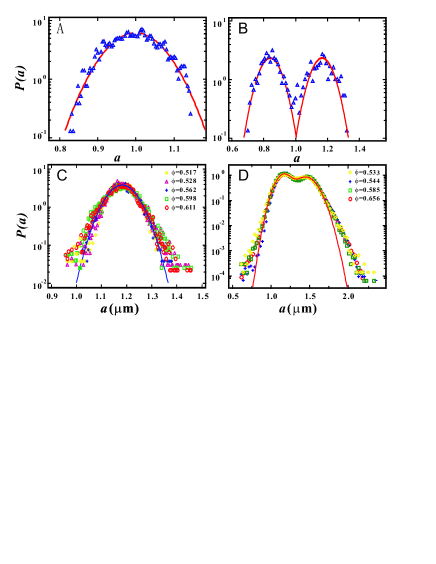
Figure 3: (color online) Particle size distributions. (A) The distribution of the true radius (solid lines) and the estimated radius $a_{i}^{(10)}$ (triangles) for a simulated nominally monodisperse sample with $\phi=0.51$ and polydispersity $p=0.07$. (B) The distribution of the true radius (solid lines) and the estimated radius $a_{i}^{(10)}$ (triangles) for a simulated nominally binary sample with $\phi=0.51$; see text for more details. (C) The radii distributions for the nominally monodisperse experimental suspension from ref. EricSci , for five volume fractions as indicated. The solid line is a Gaussian fit to the combined data, giving $p=0.045$. (D) The radii distributions for the nominally binary experimental suspension from ref. Narumi , for four volume fractions as indicated. Here the solid line is a fit to the sum of two Gaussians. With the size ratio (1:1.3) and the polydispersity of each species ($p=0.049$ for the small species, $p=0.050$ for the large species), the two sub-distributions have substantial overlap.

An important use of the estimation technique is to measure the particle size distribution of a sample in situ; we wish to validate this idea with the simulation data. To do this, we compare the estimated radius distribution $P(a_{i}^{(10)})$ with the true radius distribution $P(a_{i})$ in Fig. 3A,B. In both the nominally monodisperse sample and the nominally binary sample, the estimated distribution (symbols) is quite close to the true distribution (lines). Our results show that the estimated distribution is essentially reproduced by convolving the true distribution with a Gaussian of width $\Delta a$. For a single-species sample with a Gaussian distribution of radii with polydispersity $p$, the estimated polydispersity would be $\sqrt{p^{2}+\Delta a^{2}}$. Given that for most situations we have shown $\Delta a\ll p$, our technique will only slightly increase the apparent polydispersity of a sample.

One key difference between simulations and experiments is the boundary condition. Our simulations have periodic boundaries. In an experiment, we can not find all nearest neighbors of a particle when the particle is located at the edges of an image. This situation is similar to colloidal gels, where the number of nearest neighbors varies for each particle, and we adopt the same solution used there. For each particle, we average over a number of nearest neighbors given by $Z_{i}=7c_{i}/13$, where $c_{i}$ is the observed coordination number defined before, and we round $Z_{i}$ to the nearest integer. The denominator 13 is chosen as the number of neighbors in a close-packed sample, and the numerator 7 is from the results of Fig. 1A.

Furthermore, we need one more improvement when we apply our method to a nominally binary sample. It usually happens that we know the mean radii of each of the two species, while the number ratio of two species is unknown, which means that $\bar{a}$ is unknown. In this situation, we start with a reasonable guess for $\bar{a}^{\prime}$ to be used in Eq. 3. Then we compute the particle radii and obtain the double peak distribution which depends on our guess $\bar{a}^{\prime}$. Both peak radii of the trial estimated radius distribution should be shifted by $(\bar{a}^{\prime}-\bar{a})$ from the known mean radii. Thus we subtract $(\bar{a}^{\prime}-\bar{a})$ to adjust the peak positions to the known mean radius of each species and we obtain the estimated particle size.

In an experiment we do not have an alternate means to determine each particle size and so cannot directly verify our results in the way that the simulations allow. However, evidence that our method works is shown in Fig. 3C,D. Here, we analyzed previously published experimental data from ref. EricSci (nominally monodisperse) and ref. Narumi (nominally binary). In each case, data from several different volume fractions are shown. The size distributions agree well for the different volume fractions for both the monodisperse and binary cases. Each different volume fraction was a sample taken from the same stock jar and therefore should have the same size distribution, so this is a confirmation that our method works well with experimental data.

We now demonstrate the utility of our algorithm by studying colloidal crystal nucleation. The nucleation of crystals in a dense particle suspension depends sensitively on polydispersity pusey09 ; schope07 ; henderson98 . We examine data of the $\phi=0.46$ sample from ref. Eric2002 , analyzed at longer times to examine the crystallization process that was discarded from the analysis in ref. Eric2002 . These particles are slightly charged, shifting the freezing point to $\phi_{\rm freeze}\approx 0.38$ and the melting point to $\phi_{\rm melt}\approx 0.42$ Gasser . In this data, we confirm that the crystal nucleus appears at the center of our microscopic image: this is homogeneous nucleation, not heterogeneous nucleation near the wall.

At each time step, we calculate the number of ordered neighbors $N_{o}$ for each particle using standard techniques Gasser ; Wolde [see Methods]. By convention, a crystalline particle has $N_{o}\geq 8$ Gasser ; Wolde . At each time we compute the number fraction of the sample that is crystallized, $X(t)$. Figure 4A shows $X(t)$ as a function of both individual particle size and time, where darker colors correspond to larger values of $X(t)$. Below $t=3000$ s, $X<0.2$ for all $a$, and essentially all crystal clusters are below the critical size ($\sim 100$ particles) Gasser . At $t=3000$ s, a sufficiently large crystalline region appears and begins to grow. $X$ increases first for particles with $a$ close to the mean radius, and these particles continue to be the subpopulation that is the most crystallized at any given time. At longer times the particles with $a$ farther from $\bar{a}$ gradually begin to crystallize.

We next consider an alternate way of thinking about the same data. Figure 4B shows the relationship between the sample-averaged $X(t)$ (solid black line), the polydispersity $p_{X}$ for all crystalline particles (blue circles), and the polydispersity $p_{nX}$ for all non-crystalline particles (green squares). $X$ starts to increase at $t=3000$ s, and those particles that are crystalline at that time have $p_{X}\sim 0.03$, smaller than the bulk polydispersity $p=0.045$. As the sample crystallizes we observe that both $p_{X}$ and $p_{nX}$ increase. The growth of $p_{X}$ indicates that the crystal, while nucleating in a fairly monodisperse region, can grow by incorporating particles that are farther from the mean size. In the final state, the local polydispersity of the crystalline particles has nearly reached the mean polydispersity $p$. The growth of $p_{nX}$ indicates that those particles that are still outside the crystal are more likely to be those with unusual sizes.

The spatial distribution of particles at the end of the experiment is shown in Fig. 4C,D. Figure 4C shows the locations of the crystalline particles, while D shows the locations of the non-crystalline particles. Green particles have $a_{i}$ close to $\bar{a}$, while the smallest particles are drawn blue and the largest drawn red. The cores of the crystal regions are composed of the green particles.

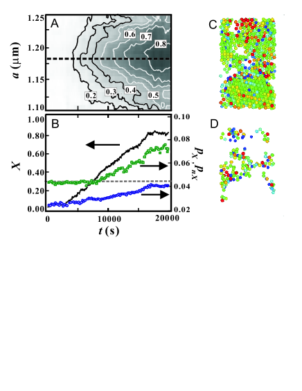
Figure 4: Relationship between individual particle size $a_{i}$ and crystallization. (A) The contour plot of the fraction of crystalline particles $X$ as a function of $a_{i}$ and time $t$. The contour lines are numbered by the value of $X$. The dashed line shows the mean radius $\bar{a}$. Particles with radii close to $\bar{a}$ crystallize faster. (B) The fraction of the sample $X$ that is crystalline as a function of time (solid black line), along with the mean polydispersity of all crystalline particles (blue circles) and all non-crystalline particles (green squares). The gray dashed line corresponds to the bulk polydispersity $p=0.045$. (C) The crystalline particles are shown at $t=20000$ s. (D) The non-crystalline particles are shown at $t=20000$ s. For C and D, the color indicates $a_{i}$ for each particle, where blue corresponds to smaller $a_{i}$, light green corresponds to $a_{i}$ close to $\bar{a}$, and red corresponds to larger $a_{i}$.

Next, we examine the beginning of the crystal nucleation process. While many particles are close to the mean size, only a few end up being the nucleation site. To understand which ones nucleate, we now focus on the particles close to the mean size: radii 1.175 $\mu$m $<a_{i}<$ 1.185 $\mu$m. Among those particles, we define the nucleus particles as those that are crystalline particles at $t=5000$ s; the remainder are non-nucleus particles. We next define the local polydispersity $p_{i}(r)$ of particle $i$ as

$$p_{i}(r)=\sqrt{\langle(a_{j}-a_{i})^{2}\rangle}/a_{i}$$ (5)

where the angle brackets $\langle\rangle$ indicate an average over all particles $j$ with centers within a distance $r$ from particle $i$. Figures 5A,B show space-time plots of the mean value of $p_{i}(r)$ for the nucleus particles (A) and the non-nucleus particles (B). In all cases, $p_{i}(r)$ is lower close to the particles and increases with increasing $r$. However, notably the contours for low $p_{i}$ are at smaller values of $r$ for the nucleus particles (A). After $t\approx 3000$ s, the region of low $p_{i}$ spreads to large values of $r$ for the nucleus particles (A), while little change is seen for the non-nucleus particles (B). Simultaneously, we show the temporal change of $N_{o}$ in Fig. 5C for the nucleus particles (solid black line) and the non-nucleus particles (dashed gray line). This confirms that the onset of crystallization at $t\approx 3000$ s coincides with the expansion of the low local polydispersity region seen in Fig. 5A. This is all evidence that crystal nuclei are formed from regions where the particles are all similar sizes. A reasonable conjecture is that nucleation rates are possibly quite sensitive to how well-mixed the sample initially is, in this respect of local polydispersity.

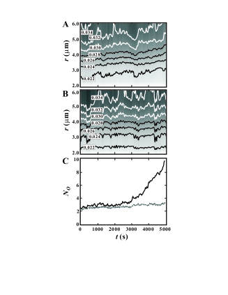
Figure 5: Relationship between nucleation properties and the local polydispersity $p_{i}(r)$. (A) The contour plot of the mean $p_{i}(r)$ as a function of $r$ and $t$, averaged over all particles which are crystalline at $t=5000$ s. The numbers on the contour lines represent the value of $p_{i}(r)$. (B) The contour plot of the mean $p_{i}(r)$ as a function of $r$ and $t$, averaged over all particles which are non-crystalline at $t=5000$ s. The particles considered in (A) and (B) are only those with radii close to the mean radii; see text for details. (C) The number of ordered neighbors $N_{o}$ as a function of time for those particles plotted in (A) (nucleus particles, solid line) and (B) (non-nucleus particles, dashed line).

We have developed a general method to estimate the particle sizes in a dense particulate samples where the particle positions are known. Simulations demonstrate the validity of our method. This method can be applied to any cases where three-dimensional particle positions can be found; while we have focused on colloidal samples, granular media are quite similar dijksman12 ; slotterback08 . We have demonstrated the utility of our method by examining homogeneous colloidal crystal nucleation. While it has been known that nucleation is faster for more monodisperse samples, we find this is true on a quite local scale. Nucleation happens in regions that are locally more monodisperse, and crystal growth is proceeds by preferentially incorporating particles close to the mean size.

Materials and Methods

We simulate four particle suspension systems, which are random close packing (RCP), colloidal gel, single component suspension, and a binary system. The polydisperse RCP sample is generated using the algorithm of ref. Xu . For the three other cases, we perform three-dimensional Monte Carlo simulations with hard spheres. Additionally for gels, we wish to model colloid-polymer mixtures and so we use the Asakura and Oosawa model AO . This model leads to a pair interaction between two hard colloidal spheres in a solution of ideal polymers as $U(r)=\infty$ for $r<\sigma_{ij}$, $U(r)=-\frac{\pi}{12}k_{B}T\rho_{p}[r^{3}-3(\sigma_{ij}+R_{G})^{2}r+2(\sigma_{ij}+R_{G})^{3}]$ for $\sigma_{ij}\leq r<\sigma_{ij}+2R_{G}$, $U(r)=0$ for $r\geq\sigma_{ij}+2R_{G}$, where $\sigma_{ij}=(\sigma_{i}+\sigma_{j})/2$, $\sigma_{i}$ is a diameter of particle $i$, $k_{B}$ is Boltzmann constant, $T$ is temperature, $\rho_{p}$ is the number density of polymers, and $R_{G}$ is the polymer radius of gyration. We fix $R_{G}=0.1\bar{\sigma}$ and $\phi_{p}=4\pi/3R_{G}^{3}\rho_{P}=0.1$ where $\bar{\sigma}$ is the mean diameter of the hard spheres. For our single-component and two-component hard sphere suspensions, particles interact via $U(r)=\infty$ for $r<\sigma_{ij}$, otherwise $U(r)=0$. We use 1024 particles with the mean radius $\bar{a}$ = 1 and variable polydispersity for all simulations.

The experimental data come from prior experiments EricSci ; Narumi . These experiments used sterically stabilized poly(methyl methacrylate) (PMMA) particles and imaged them with confocal microscopy. The particle positions were located and tracked using standard particle tracking techniques Dinsmore ; Crocker . Detailed experimental discussions are in the prior references.

We use previously developed order parameters to look for crystalline particles and ordered structure Gasser ; Wolde ; Steinhardt . For each particle $i$, we find its nearest neighbors $j$ and identify unit vectors $\hat{r}_{ij}$ pointing to the neighbors. We then define a complex order parameter $\hat{q}_{lm}$ using $q_{lm}(i)=\sum_{j=1}^{c_{i}}Y_{lm}(\hat{\bf r}_{ij})$ where $c_{i}$ is the number of nearest neighbors of particle $i$ and $Y_{lm}$ is a spherical harmonic function; we normalize this as $\hat{q}_{lm}=q_{lm}/N$ where $N$ is a normalization factor such that $\sum_{m}\hat{q}_{lm}(i)\hat{q}_{lm}^{*}(i)=1$ Gasser . We use $l=6$. For each particle pair, we compute the complex inner product $d_{6}=\sum_{m}\hat{q}_{lm}(i)\hat{q}_{lm}^{*}(j)$. Two neighboring particles are termed “ordered neighbors” if $d_{6}$ exceeds a threshold value of 0.5. For each particle, we focus on $N_{o}$, the number of ordered neighbors it has at a given time. $N_{o}^{i}$ measures the amount of similarity of structure around neighboring particles. $N_{o}^{i}$ =0 corresponds to random structure around particle $i$, while a large value of $N_{o}^{i}$ means that particle $i$ and its neighbor particles have similar surroundings Wolde .

References

- (1) Prasad, V., Semwogerere, D. & Weeks, E. R. Confocal microscopy of colloids. J. Phys.: Cond. Matt. 19, 113102 (2007).
- (2) Dijksman, J. A., Rietz, F., Lőrincz, K. A., van Hecke, M. & Losert, W. Refractive index matched scanning of dense granular materials. Rev. Sci. Inst. 83, 011301 (2012).
- (3) Pusey, P. N. & van Megen, W. Phase behaviour of concentrated suspensions of nearly hard colloidal spheres. Nature 320, 340–342 (1986).
- (4) Anderson, V. J. & Lekkerkerker, H. N. Insights into phase transition kinetics from colloid science. Nature 416, 811–815 (2002).
- (5) Vincent, B. Introduction to Colloidal Dispersions (Blackwell Publishing, 2005).
- (6) van Blaaderen, A., Imhof, A., Hage, W. & Vrij, A. Three-dimensional imaging of submicrometer colloidal particles in concentrated suspensions using confocal scanning laser microscopy. Langmuir 8, 1514–1517 (1992).
- (7) van Blaaderen, A. & Wiltzius, P. Real-space structure of colloidal hard-sphere glasses. Science 270, 1177–1179 (1995).
- (8) Kegel, W. K. & van Blaaderen, A. Direct observation of dynamical heterogeneities in colloidal Hard-Sphere suspensions. Science 287, 290–293 (2000).
- (9) Weeks, E. R., Crocker, J. C., Levitt, A. C., Schofield, A. & Weitz, D. A. Three-Dimensional direct imaging of structural relaxation near the colloidal glass transition. Science 287, 627–631 (2000).
- (10) Weeks, E. R. & Weitz, D. A. Properties of cage rearrangements observed near the colloidal glass transition. Phys. Rev. Lett. 89, 095704 (2002).
- (11) Dinsmore, A. D., Weeks, E. R., Prasad, V., Levitt, A. C. & Weitz, D. A. Three-Dimensional confocal microscopy of colloids. App. Optics 40, 4152–4159 (2001).
- (12) Narumi, T., Franklin, S. V., Desmond, K. W., Tokuyama, M. & Weeks, E. R. Spatial and temporal dynamical heterogeneities approaching the binary colloidal glass transition. Soft Matter 7, 1472–1482 (2011).
- (13) van Blaaderen, A., Ruel, R. & Wiltzius, P. Template-directed colloidal crystallization. Nature 385, 321–324 (1997).
- (14) Gasser, U., Weeks, E. R., Schofield, A., Pusey, P. N. & Weitz, D. A. Real-Space imaging of nucleation and growth in colloidal crystallization. Science 292, 258–262 (2001).
- (15) Dullens, R. P. A., Aarts, D. G. A. L. & Kegel, W. K. Dynamic broadening of the Crystal-Fluid interface of colloidal hard spheres. Phys. Rev. Lett. 97, 228301 (2006).
- (16) Dinsmore, A. D. & Weitz, D. A. Direct imaging of three-dimensional structure and topology of colloidal gels. J. Phys.: Cond. Matt. 14, 7581–7597 (2002).
- (17) Dibble, C. J., Kogan, M. & Solomon, M. J. Structure and dynamics of colloidal depletion gels: Coincidence of transitions and heterogeneity. Phys. Rev. E 74, 041403 (2006).
- (18) Gao, Y. & Kilfoil, M. L. Direct imaging of dynamical heterogeneities near the Colloid-Gel transition. Phys. Rev. Lett. 99, 078301 (2007).
- (19) Aarts, D. G. A. L., Schmidt, M. & Lekkerkerker, H. N. W. Direct visual observation of thermal capillary waves. Science 304, 847–850 (2004).
- (20) Hernández-Guzmán, J. & Weeks, E. R. The equilibrium intrinsic crystal-liquid interface of colloids. Proc. Nat. Acad. Sci. 106, 15198–15202 (2009).
- (21) Royall, C. P., Vermolen, E. C. M., van Blaaderen, A. & Tanaka, H. Controlling competition between crystallization and glass formation in binary colloids with an external field. J. Phys.: Cond. Matt. 20, 404225 (2008).
- (22) Poon, W. C. K., Weeks, E. R. & Royall, C. P. On measuring colloidal volume fractions. Soft Matter 8, 21–30 (2012).
- (23) Auer, S. & Frenkel, D. Prediction of absolute crystal-nucleation rate in hard-sphere colloids. Nature 409, 1020–1023 (2001).
- (24) Pusey, P. N. et al. Hard spheres: crystallization and glass formation. Phil. Trans. Roy. Soc. A 367, 4993–5011 (2009).
- (25) Sollich, P. & Wilding, N. B. Crystalline phases of polydisperse spheres. Phys. Rev. Lett. 104, 118302 (2010).
- (26) Kawasaki, T., Araki, T. & Tanaka, H. Correlation between dynamic heterogeneity and Medium-Range order in Two-Dimensional Glass-Forming liquids. Phys. Rev. Lett. 99, 215701 (2007).
- (27) Kurita, R. & Weeks, E. R. Glass transition of two-dimensional binary soft-disk mixtures with large size ratios. Phys. Rev. E 82, 041402 (2010).
- (28) Schöpe, H. J., Bryant, G. & van Megen, W. Effect of polydispersity on the crystallization kinetics of suspensions of colloidal hard spheres when approaching the glass transition. J. Chem. Phys. 127, 084505 (2007).
- (29) Henderson, S. I. & van Megen, W. Metastability and crystallization in suspensions of mixtures of hard spheres. Phys. Rev. Lett. 80, 877–880 (1998).
- (30) D’Haene, P. & Mewis, J. Rheological characterization of bimodal colloidal dispersions. Rheologica Acta 33, 165–174 (1994).
- (31) Pond, M. J., Errington, J. R. & Truskett, T. M. Implications of the effective one-component analysis of pair correlations in colloidal fluids with polydispersity. J. Chem. Phys. 135, 124513 (2011).
- (32) Berthier, L., Chaudhuri, P., Coulais, C., Dauchot, O. & Sollich, P. Suppressed compressibility at large scale in jammed packings of Size-Disperse spheres. Phys. Rev. Lett. 106, 120601 (2011).
- (33) Zachary, C. E., Jiao, Y. & Torquato, S. Hyperuniform Long-Range correlations are a signature of disordered jammed Hard-Particle packings. Phys. Rev. Lett. 106, 178001 (2011).
- (34) Kurita, R. & Weeks, E. R. Incompressibility of polydisperse random-close-packed colloidal particles. Phys. Rev. E 84, 030401(R) (2011).
- (35) Brujić, J. et al. 3D bulk measurements of the force distribution in a compressed emulsion system. Faraday Disc. 123, 207–220 (2003).
- (36) Crocker, J. C. & Grier, D. G. Methods of digital video microscopy for colloidal studies. J. Colloid Interf. Sci. 179, 298–310 (1996).
- (37) Asakura, S. & Oosawa, F. Surface tension of High-Polymer solutions. J. Chem. Phys. 22, 1255 (1954).
- (38) Rein ten Wolde, P., Ruiz-Montero, M. J. & Frenkel, D. Numerical calculation of the rate of crystal nucleation in a Lennard-Jones system at moderate undercooling. J. Chem. Phys. 104, 9932–9947 (1996).
- (39) Slotterback, S., Toiya, M., Goff, L., Douglas, J. F. & Losert, W. Correlation between particle motion and voronoi-cell-shape fluctuations during the compaction of granular matter. Phys. Rev. Lett. 101, 258001 (2008).
- (40) Xu, N., Blawzdziewicz, J. & O’Hern, C. S. Random close packing revisited: Ways to pack frictionless disks. Phys. Rev. E 71, 061306 (2005).
- (41) Steinhardt, P. J., Nelson, D. R. & Ronchetti, M. Bond-orientational order in liquids and glasses. Phys. Rev. B 28, 784–805 (1983).