Deep Inelastic Scattering from Holographic Spin-One Hadrons

Ezequiel Koile, Sebastian Macaluso and Martin Schvellinger

IFLP-CCT-La Plata, CONICET and
Departamento de Física, Universidad Nacional de La Plata.
Calle 49 y 115, C.C. 67, (1900) La Plata,
Buenos Aires, Argentina.

Abstract

We study deep inelastic scattering structure functions from hadrons using different holographic dual models which describe the strongly coupled regime of gauge theories in the large $N$ limit. Particularly, we consider scalar and vector mesons obtained from holographic descriptions with fundamental degrees of freedom, corresponding to ${\cal{N}}=2$ supersymmetric and non-supersymmetric Yang-Mills theories. We explicitly obtain analytic expressions for the full set of eight structure functions, i.e., $F_{1}$, $F_{2}$, $g_{1}$, $g_{2}$, $b_{1}$, $b_{2}$, $b_{3}$, $b_{4}$, arising from the standard decomposition of the hadronic tensor of spin-one hadrons. We obtain the relations $2F_{1}=F_{2}$ and $2b_{1}=b_{2}$. In addition, we find $b_{1}\sim{\cal{O}}(F_{1})$ as suggested by Hoodbhoy, Jaffe and Manohar for vector mesons. Also, we find new relations among some of these structure functions.

1 Introduction

There are holographic dual models based on type IIA and type IIB string theories which describe certain aspects of strong interactions when matter fields transforming under the fundamental representation of the gauge group are taken into account [1, 2, 3, 4, 5]. In these D-brane constructions mesons are modeled as fluctuations of flavour branes in the probe approximation. From some of these models it is possible to derive properties of mesons such as ratios of masses, decay constants and the chiral Lagrangian, among others. This makes the alluded models interesting for investigating certain aspects of the phenomenology of strong interactions. Mesons derived from this kind of models are generically known as holographic mesons. One further important and very interesting question that one may ask in the context of these models is about the structure of the holographic mesons, when they are probed by virtual photons in deep inelastic scattering (DIS) processes.

The DIS cross section is proportional to the Lorentz contraction of a leptonic tensor, entirely computed within perturbative quantum field theory, and a hadronic tensor $W_{\mu\nu}$ which receives contributions from the strong coupling regime of QCD. The hadronic tensor is computed using the optical theorem, and is recast in terms of the two-point correlation function of electromagnetic currents inside the scattered hadron. From the most general Lorentz decomposition of this tensor the so-called structure functions can be extracted. In this work we shall be focussed on DIS from mesons. Spin-zero mesons have only two structure functions called $F_{1}$ and $F_{2}$. In addition, polarized spin-one hadrons have eight structure functions [6], as we shall review in the next section.

From the point of view of the gauge/string duality [7, 8, 9], Polchinski and Strassler [10] proposed a method for deriving the hadronic tensor and the DIS structure functions for glueballs and spin-$\frac{1}{2}$ hadrons, focussing on confining gauge theories that are conformal (or nearly conformal) at momenta well above the confinement scale $\Lambda$. For instance, one can think of the ${\cal{N}}=1^{*}$ SYM theory [11, 12], that can be obtained from the ${\cal{N}}=4$ SYM theory explicitly broken at a certain mass scale to pure ${\cal{N}}=1$ SYM theory. Further developments have applied the ideas of [10] to scalar mesons, unpolarized vector mesons [13, 14] and nucleons [15, 16]. On the other hand, DIS structure functions [17] and lepton-pair photo-production rates [18] have also been studied in the strong coupling regime of an ${\cal{N}}=4$ SYM plasma using a holographic dual description to obtain correlation functions of two electromagnetic currents. More recently, it has been considered ${\cal{O}}(\alpha^{\prime 3})$ corrections from type IIB string theory on DIS [19], plasma photoemission [20], as well as other plasma properties which rely on the computation of two-point correlation functions of electromagnetic currents such as the electrical conductivity [21, 22].

In this paper we investigate DIS from polarized spin-one mesons and obtain the DIS structure functions by extending the proposal of [10]. We derive the interactions in the bulk directly from the expansion up to quadratic order in the derivatives of the fields of the Dirac-Born-Infeld action of the flavour branes in the probe approximation for the D3-D7-brane model [1] and the $\textmd{D4-D8-}\overline{\textmd{D8}}$-brane model [5]. The derivation we use, which is very different from the one presented in [13, 14], is totally general and can be applied to other holographic dual models and for different holographic hadrons. We also obtain the corresponding DIS structure functions for scalar mesons using these models.

The main difference with [13, 14] is the way we construct the interaction in the bulk. So, let us summarize the method we use in this paper. The holographic dual models we consider have an internal Einstein manifold which contains a sphere: i.e. the D3-D7 brane model has an $S^{3}$ and the Sakai-Sugimoto model has an $S^{4}$. The isometry groups are $SO(4)$ and $SO(5)$, respectively. We can consider a $U(1)$ subgroup of these isometry groups. From the point of view of the dual gauge theory, these global bosonic symmetries correspond to the $R$-symmetry group $SU(2)_{R}$ in the D3-D7 brane model, while for the Sakai-Sugimoto model this corresponds to the global symmetry group $SO(5)$. Now, consider a field in the probe-brane world-volume in each of these models. Its wave function can be factorized as the product of a plane-wave in the four-dimensional Minkowski spacetime times a function depending on the radial coordinate, times a spherical harmonic on the corresponding sphere. Notice that this spherical harmonic satisfies an eigenvalue equation, with eigenvalue equal to the charge under the referred global symmetry, let us call it ${\cal{Q}}$. Also, recall that for each global continuous symmetry there is a corresponding conserved Noether’s current. This is the situation in the bulk. Now, suppose we insert a $U(1)$ current at the boundary theory, this induces a fluctuation on the boundary conditions of the bulk fields coupled to this current at the boundary. The fluctuation propagates in the bulk. The precise form of this fluctuation comes from the fact that this boundary current is a Lorentz vector which couples to the boundary value of a gauge field propagating in the bulk. As we shall explain later, this is an off-diagonal fluctuation on the bulk metric of the form $\delta g_{mj}=A_{m}(y,r)v_{j}(\Omega)$, where $A_{m}$ is the gauge field and $v_{j}$ is the Killing vector corresponding to the isometry subgroup $U(1)\subset SO(n+1)$ of the $S^{n}$ of each considered model. In this way, it is natural to straightforwardly construct the interaction Lagrangian in the bulk by coupling the bulk Noether’s current above to the gauge field $A_{m}$ with a strength given by the charge ${\cal{Q}}$. So, this is the main point in the construction that follows here. The existence of the bulk conserved Noether’s current is crucial in this construction.

The main new results we present in this paper can be summarized as follows. We develop a consistent method to derive the interaction Lagrangian from the Dirac-Born-Infeld action of flavour probe branes. Then, we obtain the full set of structure functions for scalar and polarized vector mesons in both holographic dual models. In addition, we find a completely new full tower of vector mesons from the Sakai-Sugimoto model. The reason to use these two very different holographic dual models with flavours to study deep inelastic scattering from polarized spin-one hadrons is to be able to compare the structure functions and discuss their model-dependent as well as model-independent properties. We have obtained analytic expressions for the full set of eight structure functions: $F_{1}$, $F_{2}$, $g_{1}$, $g_{2}$, $b_{1}$, $b_{2}$, $b_{3}$, $b_{4}$, which come from the standard decomposition of the hadronic tensor of spin-one hadrons. They are functions of two independent dimensionless kinematical variables: $x$ (the Bjorken parameter) and $t$, both to be defined in the next section. Indeed, we show that these functions split into a model-dependent factor, which is common to the eight structure functions of each model, and a model-independent one. We discuss model-independent properties of the structure functions, such as the relations $2F_{1}(x)=F_{2}(x)$ and $2b_{1}(x)=b_{2}(x)$, which we have obtained for all values of the Bjorken parameter (neglecting terms proportional to $t$), though the supergravity approximation only holds for values of $x$ close to one. We have found a missing $x$-factor in comparison with the usual Callan-Gross relations. This is due to the fact that, within the pure supergravity description, lepton scattering is produced from the entire hadron [10]. Also, we have found the relation $b_{1}(x)=3F_{1}(x)$ in agreement with the expectations from [6] for the $\rho$-meson, as well as an additional set of new relations among some of these structure functions that we explain in the last section of the paper.

In Section 2 we describe the kinematics of the DIS from polarized spin-one mesons which shall be relevant for our studies in the following sections. In Section 3 we very briefly review the proposal of reference [10]. In Section 4 we begin with a brief review of the D3-D7-brane model description following [1] and we show the expressions for the scalar and vector mesons. Then, we develop a consistent method to obtain the interaction Lagrangian between the mesons and the gauge field which arises from the fluctuation of the metric induced by the insertion of a current at the boundary of the spacetime. We obtain the hadronic tensor and the corresponding eight DIS structure functions from polarized spin-one vector mesons of the dual ${\cal{N}}=2$ gauge theory. In Section 5, we carry out a similar programme for the Sakai-Sugimoto model [5] using our method to derive the interaction Lagrangian from first principles. We have also obtained a full tower of vector fluctuations of the D8-brane, which has an additional quantum number, $\ell$, compared to the mesons considered in [5], that comes from the expansion on spherical harmonics on $S^{4}$. Besides, due to the fact that the DIS relevant bulk interaction region corresponds to large values of the four-dimensional energy, we consider the metric for that specific region. This allows us to calculate full analytic expressions for these mesons depending on the nine coordinates on the D8-brane. We extensively discuss our results in the last section of the paper.

2 Kinematics of DIS from spin-one hadrons

Deep inelastic scattering is a high energy process which allows to investigate the hadronic structure. Typically, a lepton is scattered from a hadron in a kinematical regime where the hadron becomes fragmented in many particles which are not measured. The process can be described as the electromagnetic scattering of a lepton by a quark or a parton inside the hadron. In this section we follow the conventions of Manohar [27], except for the four-dimensional Minkowski metric that we take as $\eta_{\mu\nu}\equiv\textmd{diag}(-1,+1,+1,+1)$. So, let us briefly summarize the kinematics of DIS from vector and scalar mesons following the quantum field theory analysis from references [27] and [6].

Let us consider an incoming lepton beam with four-momentum $k^{\mu}$ (where $k^{0}\equiv E$) which will be scattered from a fixed hadronic target. The four-momentum of the scattered lepton $k^{\prime\mu}$ (with $k^{\prime 0}\equiv E^{\prime}$) is measured, but the final hadronic state (that we call $X$) is not. The lepton exchanges a virtual photon of four-momentum $q^{\mu}$ with the initial hadronic state. The virtual photon probes the hadron at distances as small as $1/\sqrt{q^{2}}$. If the hadron is not fragmented the scattering is called elastic, otherwise the resulting process is DIS.

The DIS amplitude is given by:

$$i{\cal{M}}=(-ie)^{2}\left(\frac{-i\eta_{\mu\nu}}{q^{2}}\right)\langle k^{\prime}|J^{\mu}_{l}(0)|k,s_{l}\rangle\langle X|J^{\nu}_{h}(0)|P,h\rangle\,,$$ (1)

where $e$ is the lepton electric charge, $s_{l}$ is the polarization of the incoming lepton, $h$ is the polarization of the hadronic initial state, and $J^{\mu}_{l},\,J^{\nu}_{h}$ are the electromagnetic currents of the lepton and hadron, respectively. The polarization $h$ can be chosen as the spin in the direction of an arbitrary axis, usually the direction of the incident beam. The differential DIS cross section is then

$$d\sigma = \sum_{X}\int\frac{d^{3}k^{\prime}}{(2\pi)^{3}2E^{\prime}}(2\pi)^{4}\delta^{4}(k+P-k^{\prime}-P_{X})\frac{|{\cal{M}}|^{2}}{(2E)(2M)(v_{rel}=1)}$$

$$= \sum_{X}\int\frac{d^{3}k^{\prime}}{(2\pi)^{3}2E^{\prime}}\frac{(2\pi)^{4}\delta^{4}(k+P-k^{\prime}-P_{X})}{(2E)(2M)}\frac{e^{4}}{q^{4}}$$

$$\times\langle P,h|J^{\mu}_{h}(0)|X\rangle\langle X|J^{\nu}_{h}(0)|P,h\rangle\langle k,s_{l}|J_{l\mu}(0)|k^{\prime}\rangle\langle k^{\prime}|J_{l\nu}(0)|k,s_{l}\rangle\,,$$

where $P^{\mu}$ and $P_{X}^{\mu}$ are the hadronic initial and final momentum. $M^{2}=-P^{2}$ and $M_{X}^{2}=-P_{X}^{2}$ are the initial and final hadronic squared masses, respectively. The relation $\langle\alpha|J^{\mu}|\beta\rangle^{*}=\langle\beta|J^{\mu}|\alpha\rangle$ has been used, since $J^{\mu\dagger}=J^{\mu}$. Notice that since the polarizations of the final lepton and hadron states are not measured there is a sum over them.

The leptonic tensor is defined as

$$l^{\mu\nu}=\sum_{final\ spin}\langle k^{\prime}|J_{l}^{\nu}(0)|k,s_{l}\rangle\langle k,s_{l}|J_{l}^{\mu}(0)|k^{\prime}\rangle\,,$$ (3)

and can be computed pertubatively within quantum electrodynamics. For a spin-$\frac{1}{2}$ lepton it is given by

$$l^{\mu\nu}=2[k^{\mu}k^{\prime\nu}+k^{\nu}k^{\prime\mu}-\eta^{\mu\nu}(k\cdot k^{\prime}-m_{l}^{2})-i\epsilon^{\mu\nu\alpha\beta}q_{\alpha}s_{l\beta}],$$ (4)

where $m_{l}$ is the lepton mass.

On the other hand, the hadronic tensor $W_{\mu\nu}$ is given by [27]

$$W_{\mu\nu}(P,q)_{h^{\prime}\,h}=\frac{1}{4\pi}\int d^{4}x\,e^{iq.x}\langle P,h^{\prime}|[J_{\mu}(x),J_{\nu}(0)]|P,h\rangle\,,$$ (5)

where $h$ and $h^{\prime}$ are the polarizations of the initial and final hadronic states, respectively. By inserting a complete set of eigenstates and taking into account translational invariance, the above expression becomes

$$W_{\mu\nu}(P,q)_{h^{\prime}\,h}=\frac{1}{4\pi}\sum_{X}\bigg{[}(2\pi)^{4}\delta^{4}(q+P-P_{X})\langle P,h^{\prime}|J_{\mu}(0)|X\rangle\langle X|J_{\nu}(0)|P,h\rangle$$

$$-(2\pi)^{4}\delta^{4}(q-P+P_{X})\langle P,h^{\prime}|J_{\nu}(0)|X\rangle\langle X|J_{\mu}(0)|P,h\rangle\bigg{]}\,.$$ (6)

The allowed final states must satisfy the condition $P_{X}^{0}\geq P^{0}$, since $M_{X}^{2}\geq M^{2}$. Since $q^{0}>0$, only the first delta function in Eq.(2) fulfills this condition, thus the sum in $W_{\mu\nu}$ reduces to Eq.(2). Finally, one gets

$$\frac{d^{2}\sigma}{dE^{\prime}d\Omega}=\frac{e^{4}}{16\pi^{2}q^{4}}\frac{E^{\prime}}{ME}l^{\mu\nu}W_{\mu\nu}(P,q)_{h^{\prime}\,h}\,.$$ (7)

It is important to notice from Eq.(4) that the spin-independent part of the leptonic tensor is symmetric under $\mu\leftrightarrow\nu$, while its spin-dependent part is antisymmetric. Therefore, an unpolarized lepton beam only probes the symmetric part of the hadronic tensor $W_{\mu\nu}$.

The relevant hadronic structure for DIS can be completely characterized by $W_{\mu\nu}$. The probability that a hadron contains a given constituent with a given fraction $x$ of its total momentum is given by the partonic distribution functions, which unfortunately cannot be computed with perturbative QCD. This is because they depend on soft (non-perturbative) QCD dynamics which determines the hadronic structure as a confined state of quarks and gluons. Therefore, the incoming lepton gets scattered from the hadronic constituents which carry a fraction $x$ of the total hadronic momentum.

For the hadrons composed by massless partons the probability of finding a parton with a momentum $xP^{\mu}$ is given by the distribution function $f(x,q^{2})$. When the partons are free, this function becomes independent of $q^{2}$, i.e. $f\equiv f(x)$, which is the so-called Bjorken scaling. Obviously, this scaling does not hold for QCD where the partonic distribution functions change as a function of $q^{2}$, since each parton tends to fragment into multiple partons with lower $x$. Thus, the hadronic structure in QCD does depend on $q^{2}$, being the parton number increased while the average value of $x$ decreases as $q^{2}$ increases.

Now, let us focus upon the hadronic structure functions. First, let us review a few basic properties. They are dimensionless functions depending on $P^{2}$, $P\cdot q$ and $q^{2}$. It is useful to write them in terms of the dimensionless variables $t\equiv\frac{P^{2}}{q^{2}}$ and $x\equiv-\frac{q^{2}}{2P\cdot q}$. The ranges of these variables are $0<x\leq 1$ and $t<0$. The structure functions are obtained from the most general Lorentz decomposition of the hadronic tensor, satisfying certain physical requirements for $W_{\mu\nu}$. For parity preserving interactions it is necessary to satisfy current conservation $\partial_{\mu}J^{\mu}(x)=0$ which implies that

$$q^{\mu}W_{\mu\nu}(P,q,h)=q^{\nu}W_{\mu\nu}(P,q,h)=0\,.$$ (8)

It must also be parity invariant:

$$W_{\mu\nu}(P,q,h)=W_{\mu_{\textmd{p}}\nu_{\textmd{p}}}(P_{\textmd{p}},q_{\textmd{p}},h_{\textmd{p}})\,,$$ (9)

where the subindex p indicates parity-transformed quantities. Time-reversal symmetry must also be satisfied, which means that

$$W_{\mu\nu}(P,q,h)=W^{*}_{\nu_{T}\mu_{T}}(P_{T},q_{T},h_{T})\,,$$ (10)

where the subindex $T$ means time reversal. In addition, there is an identity relating $W_{\mu\nu}$ for $q^{0}>0$ with $W_{\mu\nu}$ for $q^{0}<0$:

$$W_{\mu\nu}(P,q,h)=-W_{\nu\mu}(P,-q,h)\,,$$ (11)

which comes from translation invariance. At this point we introduce the hadronic tensor for polarized spin-one hadrons for parity-preserving interactions as derived in [6] by Hoodbhoy, Jaffe and Manohar. There are four new structure functions in comparison with spin-$\frac{1}{2}$ hadrons, which are called $b_{1}$, $b_{2}$, $b_{3}$ and $b_{4}$. They contribute to the symmetric part of $W_{\mu\nu}$, thus contributing to DIS from an unpolarized target. Therefore, the hadronic tensor can be written in terms of eight independent structure functions. Omitting terms containing $q_{\mu}$ and $q_{\nu}$, since they vanish after the contraction with the leptonic tensor, the hadronic tensor reads

$$W_{\mu\nu} = F_{1}\eta_{\mu\nu}-\frac{F_{2}}{P\cdot q}P_{\mu}P_{\nu}+b_{1}r_{\mu\nu}-\frac{b_{2}}{6}(s_{\mu\nu}+t_{\mu\nu}+u_{\mu\nu})-\frac{b_{3}}{2}(s_{\mu\nu}-u_{\mu\nu})$$

$$-\frac{b_{4}}{2}(s_{\mu\nu}-t_{\mu\nu})-\frac{ig_{1}}{P\cdot q}\epsilon_{\mu\nu\lambda\sigma}q^{\lambda}s^{\sigma}-\frac{ig_{2}}{(P\cdot q)^{2}}\epsilon_{\mu\nu\lambda\sigma}q^{\lambda}(P\cdot q\>s^{\sigma}-s\cdot q\>P^{\sigma})\,,$$

where we have used the following definitions:

$$r_{\mu\nu}\equiv\frac{1}{(P\cdot q)^{2}}\bigg{(}q\cdot\zeta^{*}\>q\cdot\zeta-\frac{1}{3}(P\cdot q)^{2}\kappa\bigg{)}\eta_{\mu\nu}\,,$$ (13)

$$s_{\mu\nu}\equiv\frac{2}{(P\cdot q)^{3}}\bigg{(}q\cdot\zeta^{*}\>q\cdot\zeta-\frac{1}{3}(P\cdot q)^{2}\kappa\bigg{)}P_{\mu}P_{\nu}\,,$$ (14)

$$t_{\mu\nu}\equiv\frac{1}{2(P\cdot q)^{2}}\bigg{(}q\cdot\zeta^{*}\>P_{\mu}\zeta_{\nu}+q\cdot\zeta^{*}\>P_{\nu}\zeta_{\mu}+q\cdot\zeta\>P_{\mu}\zeta^{*}_{\nu}+q\cdot\zeta\>P_{\nu}\zeta^{*}_{\mu}-\frac{4}{3}(P\cdot q)P_{\mu}P_{\nu}\bigg{)}\,,$$

(15)

$$u_{\mu\nu}\equiv\frac{1}{P\cdot q}\bigg{(}\zeta^{*}_{\mu}\zeta_{\nu}+\zeta^{*}_{\nu}\zeta_{\mu}+\frac{2}{3}M^{2}\eta_{\mu\nu}-\frac{2}{3}P_{\mu}P_{\nu}\bigg{)}\,,$$ (16)

$$s^{\sigma}\equiv\frac{-i}{M^{2}}\epsilon^{\sigma\alpha\beta\rho}\zeta^{*}_{\alpha}\zeta_{\beta}P_{\rho}\,,$$ (17)

being $\kappa=1-4x^{2}t$ and $s^{\sigma}$ a four-vector analogous to the spin four-vector for spin-$\frac{1}{2}$ particles. Besides, $\zeta$ and $\zeta^{*}$ denote the initial and final hadronic polarization vectors, respectively. The condition $P\cdot\zeta=0$ is satisfied, and the normalization is given by $\zeta^{2}=-M^{2}$.

Recall that DIS amplitudes can be obtained from the imaginary part of the forward Compton scattering amplitudes. In particular, from the matrix element of two electromagnetic currents inside the hadron, the tensor $T_{\mu\nu}$ is defined as

$$T_{\mu\nu}=i\langle P,{\cal{Q}}|{\hat{T}}(\tilde{J}_{\mu}(q)\,J_{\nu}(0))|P,{\cal{Q}}\rangle\,,$$ (18)

where, as before, $P$ is the four-momentum of the initial hadronic state (where for brevity we have omitted its Lorentz index), $q$ is the four-momentum of the virtual photon and ${\cal{Q}}$ is the charge of the hadron. ${\hat{T}}(\hat{{\cal{O}}}_{1}\hat{{\cal{O}}}_{2})$ indicates time-ordered product between $\hat{{\cal{O}}}_{1}$ and $\hat{{\cal{O}}}_{2}$ operators. The tilde stands for Fourier transform. The tensor $T_{\mu\nu}\equiv T_{\mu\nu}(P,q,h)$ has identical symmetry properties as $W_{\mu\nu}(P,q,h)$, thus having similar Lorentz-tensor structure to $W_{\mu\nu}$. Using the optical theorem one gets

$$\textmd{Im}\,\tilde{F_{j}}=2\pi\,F_{j}\,,$$ (19)

being $\tilde{F_{j}}$ the $j$-th structure function of $T_{\mu\nu}$ and $F_{j}$ the corresponding one of $W_{\mu\nu}$.

3 A holographic dual description of DIS

Let us very briefly describe the idea presented in [10] by Polchinski and Strassler to study DIS for gauge theories that have holographic dual descriptions. Full details are explained in the original reference. Within the supergravity approximation they calculate hadronic structure functions for $x\sim 1$ (with $x<1$). In particular, they consider confining gauge theories in four dimensions such as certain deformations of ${\cal{N}}=4$ SYM, from which they study DIS from glueballs and spin-$\frac{1}{2}$ hadrons. The examples considered in that paper are UV conformal or nearly conformal. Thus, the dual string theory is defined on the $AdS_{5}\times W$ background, where $W$ can be an Einstein manifold. The metric is given by

$$ds^{2}=\frac{r^{2}}{R^{2}}\eta_{\mu\nu}dy^{\mu}dy^{\nu}+\frac{R^{2}}{r^{2}}dr^{2}+R^{2}\widehat{ds}^{2}_{W}\,,$$ (20)

where $R=(4\pi g_{s}N)^{1/4}\alpha^{\prime 1/2}$ is the $AdS_{5}$ radius when $W$ is the five-sphere. The four coordinates $y^{\mu}$ are identified with those of the gauge theory, while $r$ is the holographic radial one. Coordinates on $W$ are denoted by $\Omega$. The ten-dimensional energy scale is given by $R^{-1}$ (up to powers of the ’t Hooft coupling $\lambda=g_{YM}^{2}N\equiv 4\pi g_{s}N$, with the string coupling $g_{s}$), while the characteristic four-dimensional energy is

$$E^{(4)}\sim\frac{r}{R^{2}}\,.$$ (21)

If one is interested in the large $N$ limit of confining gauge theories, the geometry of the holographic dual model at large $r$ is approximately that of Eq.(20), however, it must be modified at a radius corresponding to

$$r\sim r_{0}=\Lambda R^{2}\,,$$ (22)

where $\Lambda$ is the confinement scale. Nevertheless, the dynamics of interest for $q\gg\Lambda$ corresponds to $r_{int}\sim qR^{2}\gg r_{0}$, where the conformal metric (20) can be used. $r_{int}$ denotes the bulk region where the relevant interaction occurs as we explain below.

Polchinski and Strassler employ the dual string theory description to obtain the matrix element $T^{\mu\nu}$. Its imaginary part is given by

$$\textmd{Im}\>T^{\mu\nu} = \pi\sum_{P_{X},X}\langle P,{\cal{Q}}|J^{\nu}(0)|P_{X},X\rangle\langle P_{X},X|\tilde{J}^{\mu}(q)|P,{\cal{Q}}\rangle\,,$$ (23)

$$= 2\pi^{2}\sum_{X}\delta(M_{X}^{2}+[P+q]^{2})\langle P,{\cal{Q}}|J^{\nu}(0)|P+q,X\rangle\langle P+q,X|J^{\mu}(0)|P,{\cal{Q}}\rangle\,.$$

The momenta $P_{\mu}$, $q_{\mu}$, the polarization $n_{\mu}$ and the currents $J_{\mu}$ are considered as four-dimensional quantities, being their Lorentz indices raised and contracted with $\eta^{\mu\nu}$.

In the large $N$ limit of the gauge theory only single hadron states will contribute. In the gauge theory for the $s$-channel we have

$$s=-(P+q)^{2}\simeq q^{2}\bigg{(}\frac{1}{x}-1\bigg{)}\,,$$ (24)

where it has been used $-P^{2}\ll q^{2}$. The corresponding ten-dimensional scale is

$$\tilde{s}=-g^{MN}P_{X,M}P_{X,N}\leq-g^{\mu\nu}(P+q)_{\mu}(P+q)_{\nu}\sim\frac{R^{2}}{r^{2}_{int}}q^{2}\bigg{(}\frac{1}{x}-1\bigg{)}=\frac{\bigg{(}\frac{1}{x}-1\bigg{)}}{\alpha^{\prime}(4\pi g_{s}N)^{1/2}}\,.$$ (25)

The ’t Hooft parameter appears in the denominator, so if $(g_{s}N)^{-1/2}\ll x<1$ we have $\alpha^{\prime}\tilde{s}\ll 1$. Therefore, for $x\sim 1$ (with $x<1$) only massless string states are produced, and we are dealing with a supergravity process [10]. This is the regime studied in the present paper.

Now, let us focus on the way that the DIS process is viewed from the bulk theory. Recall that in the four-dimensional boundary theory we have to obtain the two-point function of two electromagnetic currents inside the hadron. Using the gauge/string duality the current operator inserted at the boundary of the $AdS$ space induces a perturbation on the boundary condition of a bulk gauge field. The perturbation excites a non-normalizable mode which propagates within the bulk [8, 9]. We can see how bulk gauge fields appear as follows. The isometry group of the manifold $W$ corresponds to an R-symmetry group on the field theory. We can consider a $U(1)_{R}$ subgroup and the associated R-symmetry current can now be identified with the electromagnetic current inside the hadron. In addition, for the global symmetry group corresponding to the isometry of manifold $W$, there is a Killing vector $\upsilon_{j}$. It excites a non-normalizable mode of a Kaluza-Klein gauge field,

$$\delta g_{mj}=A_{m}(y,r)\upsilon_{j}(\Omega)\,.$$ (26)

In the case of glueballs, the holographic dual field in [10] corresponds to the dilaton. Thus, the incoming bulk dilaton field $\Phi_{i}$ couples to the bulk $U(1)$-gauge field $A_{\mu}$ (induced by a current inserted at the boundary) and to another dilaton $\Phi_{X}$, which represents an intermediate hadronic state (See Figure 1). The latter propagates in the bulk and couples to an outgoing dilaton $\Phi_{f}$ (corresponding to the final hadronic state) and a gauge field $A_{\nu}$ in the bulk which comes from the insertion of a second boundary theory current. This Witten diagram represents the holographic dual version of the optical theorem [10] for a DIS process which is schematically shown at the boundary slice, where the leptonic currents are indicated with $l$, and they couple to the virtual photons indicated by dashed lines at the boundary slice. Then, these photons couple to the currents inside the hadrons, which are indicated by solid lines on the boundary slice and are labeled by the momenta carried by the initial, intermediate and final hadronic states, $P_{i}$, $P_{X}$ and $P_{f}$, respectively.

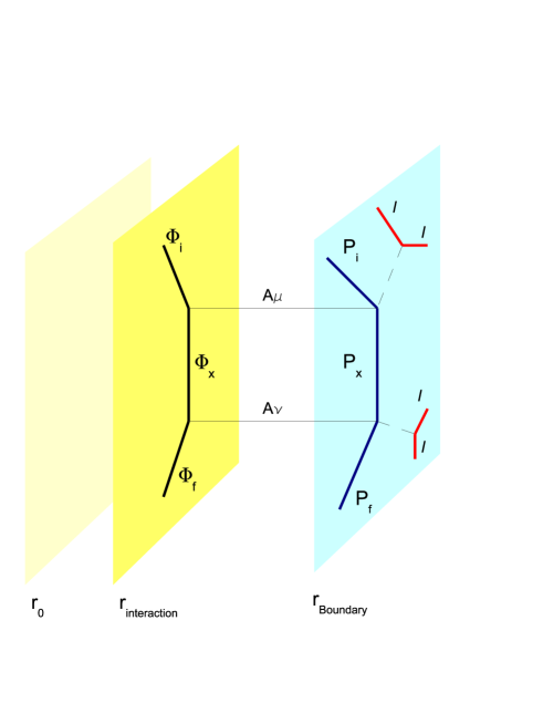
Figure 1: Schematic representation of the AdS/CFT prescription for the calculation of the tensor $T_{\mu\nu}$. The interaction in the bulk occurs at $r_{interaction}$, we also show the slices corresponding to the IR cutoff $r_{0}$ and the boundary.

The present holographic approach corresponds to a DIS process where the lepton is scattered from an entire hadron, which becomes excited but does not fragment. In the next two sections we extend these ideas to other holographic dual models.

4 DIS from mesons in the D3-D7-brane model

In this section we firstly give a brief introduction to the D3-D7-brane model developed in reference [1]. In [28] it was shown that by introducing $N_{f}$ D7-branes in the $AdS_{5}\times S^{5}$ background of type IIB string theory, it is possible to describe $N_{f}$ hypermultiplets in the gauge theory preserving ${\cal{N}}=2$ supersymmetries in four dimensions. The starting point is a set of coincident parallel $N$ D3-branes and $N_{f}$ D7-branes which share directions 0-3 with the former ones. The hypermultiplets in the gauge theory arise from the lightest modes of the fundamental strings extended between D3 and D7-branes: those are modes of the type 3-7 and 7-3, whose mass is $m_{q}=L/2\pi\alpha^{\prime}$, where $L$ is the distance between D3 and D7-branes in the (8, 9) plane. In the decoupling limit of the D3-branes, namely $g_{s}N\gg 1$ where $g_{s}$ is the string coupling, the background becomes $AdS_{5}\times S^{5}$. Also, if $N\gg N_{f}$ then the backreaction of the D7-branes can be neglected. In these limits the description corresponds to $N_{f}$ probe D7-branes in the referred $AdS_{5}\times S^{5}$ geometry. We consider only the Abelian case ($N_{f}=1$), which implies the existence of a global $U(1)$ symmetry group, associated with the flavour symmetry of the ${\cal{N}}=2$ $SU(N)$ SYM theory. This theory has dynamical quarks, thus it is very interesting to investigate the DIS structure of scalar and vector mesons which arise from this model. We should be aware that this model does not allow to describe spontaneous breaking of chiral symmetry. This makes a difference with respect to QCD and the Sakai-Sugimoto model [5]. In [1] the mass spectra for different types of mesons have been computed through its holographic dual description. In this work we shall obtain the structure functions of the hadronic tensor for DIS from those scalar and polarized vector mesons.

We develop a systematic method to derive the interaction Lagrangian ${\cal{L}}_{int}$ in the holographic dual theory, in a complementary way with respect to the proposal of Polchinski and Strassler [10]. We emphasize that the interaction Lagrangian obtained using both methods is the same for the case studied by Polchinski and Strassler [10], while it gives very different results for vector mesons in comparison with [13] and [14]. The present approach guarantees the existence of a conserved current in eight dimensions straightforwardly derived from the Dirac-Born-Infeld action. From this current we shall see that the property $q_{\mu}W^{\mu\nu}=0$ is satisfied. Moreover, we have checked that ${\cal{L}}_{int}$ is invariant under parity and time-reversal transformations. Thus, the hadronic tensor automatically satisfies the properties indicated in Eqs.(8)-(11). All these are consistency checks that confirm the correctness of the procedure we develop here. Next step will be the derivation of the structure functions for scalar and polarized vector mesons, obtaining analytical expressions for all of them.

The D3-D7-brane model

For this brief subsection we follow reference [1]. Let us consider a type IIB string theory background consisting of $N$ coincident D3-branes. This corresponds to the geometry $AdS_{5}\times S^{5}$ whose metric is

$$ds^{2}=\frac{r^{2}}{R^{2}}\>ds^{2}({E}^{(1,3)})+\frac{R^{2}}{r^{2}}d\vec{Z}\cdot d\vec{Z}\,,$$ (27)

where the coordinates $Z^{i}$, $i=1,\ldots,6$ parameterize the transversal directions to the D3-branes and $r=\big{|}\vec{Z}\big{|}$. In addition, the $AdS_{5}$ radius is given by $R^{2}=\sqrt{4\pi g_{s}N}\alpha^{\prime}$.

Let us add a probe D7-brane at a certain distance $|\vec{Z}|=L$ from the D3-branes in the (8, 9) plane. In this case the hypermultiplet becomes massive, and the R-symmetry is $SU(2)_{R}$. The induced metric on the D7-brane is

$$ds^{2}=\frac{\rho^{2}+L^{2}}{R^{2}}\>ds^{2}({E}^{(1,3)})+\frac{R^{2}}{\rho^{2}+L^{2}}d\rho^{2}+\frac{R^{2}\rho^{2}}{\rho^{2}+L^{2}}d\Omega_{3}^{2}\,,$$ (28)

where $\rho^{2}=r^{2}-L^{2}$ and $\Omega_{3}$ are the spherical coordinates in the space spanned by the coordinates 4-7. For $L=0$ the metric reduces to $AdS_{5}\times S^{3}$, rendering a conformal gauge theory. On the other hand, if $L\neq 0$, the above metric is only asymptotically $AdS_{5}\times S^{3}$ for $\rho\gg L$. This shows the explicit breaking of conformal invariance induced by the hypermultiplet mass $m_{q}=L/2\pi\alpha^{\prime}$, which is recovered in the high energy limit, $E\gg m_{q}$. Notice that the radius of the $S^{3}$ is not a constant, and moreover it goes to zero for $\rho=0$ (which corresponds to $r=L$), where the D7-brane ends as seen from the projection on the $AdS_{5}$.

In [1] the spectra of scalar and vector mesons were computed, and they were arranged in supersymmetric multiplets which transform according to representations of the global $SU(2)_{R}\times SU(2)_{L}$ symmetry group. These mesons correspond to excitations of open strings of the D7-brane. The dynamics of the probe D7-brane fluctuations is described in terms of the following action

$$S_{D7} = -\mu_{7}\int d^{8}\xi\sqrt{-\textmd{det}(P[g]_{ab}+2\pi\alpha^{\prime}F_{ab})}+\frac{(2\pi\alpha^{\prime})^{2}}{2}\mu_{7}\int P[C^{(4)}]\wedge F\wedge F\,,$$ (29)

$g_{ab}$ stands for the metric (28), $\mu_{7}=[(2\pi)^{7}g_{s}\alpha^{\prime 4}]^{-1}$ is the D7-brane tension and $P$ denotes the pullback of the background fields on the D7-brane world-volume. The relevant part of the Ramond-Ramond potential in the Wess-Zumino term is

$$C^{(4)}=\frac{r^{4}}{R^{4}}dy^{0}\wedge dy^{1}\wedge dy^{2}\wedge dy^{3}\,.$$ (30)

Next, in order to fix our notation and give a self-contained derivation of the hadronic tensor, we show briefly how the mesons are obtained from the present model. Then, we carry out the derivation of the hadronic tensor and the structure functions for scalar and vector mesons.

DIS from scalar mesons

The equations of motion for scalar mesons are obtained from transversal fluctuations of the D7-brane [1]

$$Z^{5}=0+2\pi\alpha^{\prime}\chi\,,\>\>\>\>\>\>\>\>\>\>\>\>\>\>\>Z^{6}=L+2\pi\alpha^{\prime}\varphi\,,$$ (31)

where the coordinates $Z^{5}$ and $Z^{6}$ lie on the (8, 9) plane, transversal to the D7-brane. $\chi$ and $\varphi$ are the scalar fluctuations whose Lagrangian is straightforwardly derived from action (29),

$${\mathcal{L}}=-\mu_{7}\sqrt{|{\det}(g_{ab})|}\sqrt{\det(\delta^{ab}+(g^{ac}R^{2}/r^{2})(2\pi\alpha^{\prime})^{2}(\partial_{c}\chi\partial^{b}\chi+\partial_{c}\varphi\partial^{b}\varphi))}\,.$$ (32)

All indices denote directions in the world-volume of the D7-brane. Expanding the above Lagrangian up to quadratic order in the derivatives of the fluctuations, the previous equation becomes

$${\mathcal{L}}=-\mu_{7}\sqrt{|\det(g_{ab})|}\bigg{[}1+\frac{2R^{2}}{r^{2}}g^{ab}(\pi\alpha^{\prime})^{2}(\partial_{b}\chi\partial_{a}\chi+\partial_{b}\varphi\partial_{a}\varphi)\bigg{]}\,,$$ (33)

which only depends upon derivatives of the scalars. The D7-brane wraps the $S^{3}$, whose radius is denoted by $\rho$. Substituting $r^{2}=\rho^{2}+L^{2}$ and the metric (28) in the quadratic Lagrangian one obtains the equations of motion (EOM) for scalar fluctuations of the D7-brane in the probe approximation, which reads

$$\partial_{a}\bigg{(}\frac{\rho^{3}\sqrt{\textmd{det}\tilde{g}}}{\rho^{2}+L^{2}}g^{ab}\partial_{b}\Phi\bigg{)}=0\,,$$ (34)

where $\Phi$ is either fluctuation ($\chi$ or $\varphi$), while $\tilde{g}_{ij}$ is the metric of a 3-sphere of unit radius, which together with $\rho$ include the directions ($Z^{1}$, $\cdots$, $Z^{4}$). The EOM can be written more explicitly as

$$\frac{R^{4}\rho}{(\rho^{2}+L^{2})}\delta^{\mu\nu}\partial_{\mu}\partial_{\nu}\Phi+\partial_{\rho}\bigg{(}\frac{\rho^{5}}{(\rho^{2}+L^{2})}\partial_{\rho}\Phi\bigg{)}+\frac{\rho^{3}}{(\rho^{2}+L^{2})}\nabla^{i}\nabla_{i}\Phi=0\,,$$ (35)

where $\nabla_{i}$ is the covariant derivative on $S^{3}$. Indices $a$, $b$, $c$, $\cdots$ denote coordinates on the D7-brane world-volume; $i$, $j$, $k$, $\cdots$ are on $S^{3}$; $\mu$, $\nu$, $\cdots$ indicate directions parallel to the D3-branes and $m$, $n$, $\cdots$ correspond to $0,1,2,3,\rho$ coordinates.

Now, we need the wave functions for the scalar mesons in a region where

$$r_{int}=\sqrt{\rho_{int}^{2}+L^{2}}\sim qR^{2}\gg r_{0}\equiv\Lambda R^{2}>\sqrt{2}L\>\>\Rightarrow\>\>\rho_{int}\gg L\,,$$ (36)

where $r_{int}$ denotes the interaction region and $\Lambda$ is an infrared cutoff for the four-dimensional gauge theory. In this region the metric can be approximated by $AdS_{5}\times S^{3}$, which reflects the fact that for energies as high as $E\gg m_{q}$ the explicitly broken conformal invariance gets restored. Thus, the resulting EOM is

$$\frac{R^{4}}{\rho}\delta^{\mu\nu}\partial_{\mu}\partial_{\nu}\Phi+\partial_{\rho}(\rho^{3}\partial_{\rho}\Phi)+\rho\nabla^{i}\nabla_{i}\Phi=0\,.$$ (37)

The proposed Ansatz for the solution is

$$\Phi^{\ell}=\phi(\rho)\>e^{iP\cdot y}\>Y^{\ell}(S^{3})\,,$$ (38)

where $Y^{\ell}(S^{3})$ are the scalar spherical harmonics on $S^{3}$, which satisfy the eigenvalue equation

$$\nabla^{i}\nabla_{i}Y^{\ell}(S^{3})=-\ell(\ell+2)Y^{\ell}(S^{3})\,.$$ (39)

Notice that in order to simplify the notation, from now on we will call $\Phi\equiv\Phi^{\ell}$, omitting the $\ell$ index.

Thus, the Lagrangian (33) for the complex scalar $\Phi$ in the interaction region can be written as

$${\mathcal{L}}=-\mu_{7}(\pi\alpha^{\prime})^{2}\sqrt{|\textmd{det}g|}\frac{R^{2}}{\rho^{2}}g^{ab}(\partial_{a}\Phi\partial_{b}\Phi^{*}+\partial_{b}\Phi\partial_{a}\Phi^{*})\,.$$ (40)

Now, we have to derive the EOM for the fields in the $AdS$ space. Thus, replacing the solution (38) for the scalar mesons in the interaction region defined by Eq.(36), we obtain

$$\partial_{\rho}^{2}\phi+3\rho^{-1}\partial_{\rho}\phi+(-P^{2}R^{4}\rho^{-4}-m^{2}_{\ell}\rho^{-2})\phi=0\,,$$ (41)

with $m^{2}_{\ell}=\ell(\ell+2)$.

For the initial/final hadronic state (IN/OUT), with four-momentum $P$, we can use the leading behaviour of the solution in the region $\rho\sim\rho_{int}$, while for the intermediate state $X$ with four-momentum $P_{X}$, we have to use the full solution. Thus, we obtain

$$\Phi_{IN/OUT}=c_{i}(\Lambda\rho)^{-\nu-1}e^{iP\cdot y}Y(\Omega)\,,$$ (42)

$$\Phi_{X}=c_{X}\Lambda^{-3/2}s^{1/4}\rho^{-1}J_{\nu}\bigg{(}\frac{s^{1/2}R^{2}}{\rho}\bigg{)}e^{iP_{X}\cdot y}Y(\Omega)\,,$$ (43)

where $J_{\nu}$ is the Bessel function of first kind, $\nu=\sqrt{m^{2}_{\ell}+1}=\ell+1$ and $s=-(P+q)^{2}=M_{X}^{2}$ is the mass-squared of the intermediate state, while $c_{X}$ and $c_{i}$ are dimensionless constants. In order to study the parity we need to use the property $[Y^{\ell}(\Omega)]_{\textmd{P}}=(-1)^{\ell}Y^{\ell}(\Omega)$. As a result, the mesons are scalar and pseudoscalar mesons for even and odd values of $\ell$, respectively.

At this point we have all the ingredients to calculate the hadronic tensor using the holographic dual prescription. For this purpose we first consider that the holographic meson couples to a gauge field in the bulk of the string theory dual model. In order to understand this coupling let us consider the insertion of a $U(1)$-current at the $AdS_{5}$ boundary. This induces a perturbation on the boundary conditions and excites a non-normalizable mode $A_{m}$ in the $AdS_{5}$ interior. This mode corresponds to the extension towards the $AdS$-interior of the $A_{\mu}|_{4d}$ field, which is in fact its boundary value. The perturbation propagates inside the $AdS$, inducing a metric fluctuation which is the product of the gauge field $A_{m}(y,\rho)$ and a Killing vector $\upsilon_{j}$ corresponding to an isometry of the internal space $S^{3}$. Thus, we consider the fluctuation proposed in [10]. Perturbing the metric in Eq.(40) we have $g^{ab}\rightarrow g^{ab}-\delta g^{ab}$, where $\delta g^{ab}=A^{m}(y,\rho)\upsilon^{j}(\Omega)$ and using $\upsilon^{j}\partial_{j}Y^{\ell}(\Omega)=i{\cal{Q}}_{\ell}Y^{\ell}(\Omega)$ (below we shall drop the $\ell$ label from the spherical harmonics and from ${\cal{Q}}_{\ell}$), the interaction Lagrangian we obtain is:

$${\mathcal{L}}_{int}=i{\cal{Q}}\mu_{7}(\pi\alpha^{\prime})^{2}\sqrt{|\textmd{det}g|}R^{2}\rho^{-2}A^{m}(\Phi\partial_{m}\Phi^{*}_{X}-\Phi^{*}_{X}\partial_{m}\Phi)\,.$$ (44)

The angular dependence on the spherical harmonics corresponds to functions which are charge eigentates, with charge ${\cal{Q}}$ under the $U(1)$ symmetry group induced by transformations on the internal $S^{3}$ in the direction of the Killing vector $\upsilon^{j}$.

Alternatively, ${\cal{L}}_{int}$ can be obtained from the coupling of the gauge field $A_{m}$ to the Noether current corresponding to the internal symmetry of the action (40) under global phase transformations associated with the $U(1)$ group, which is a subgroup of the $SO(4)$ isometry group of $S^{3}$, generated by a Killing vector $\upsilon^{j}$. The Noether’s current is:

$$j^{m}=\frac{\partial{\cal{L}}}{\partial(\partial_{m}\Phi)}\Theta+\frac{\partial{\cal{L}}}{\partial(\partial_{m}\Phi^{*})}\Theta^{*}\,.$$ (45)

Now, for an infinitesimal transformation with parameter $\vartheta/2(=\textmd{constant})$ we have

$$\delta\Phi=-i\frac{\vartheta}{2}\Phi\>\>\Rightarrow\>\>\Theta=-\frac{i}{2}\Phi\,,$$

$$\delta\Phi^{*}=i\frac{\vartheta}{2}\Phi^{*}\>\>\Rightarrow\>\>\Theta^{*}=\frac{i}{2}\Phi^{*}\,.$$ (46)

Therefore, the Noether’s current reads

$$j^{m}=i\mu_{7}(\pi\alpha^{\prime})^{2}R^{2}\rho^{-2}(\Phi\partial^{m}\Phi^{*}_{X}-\Phi^{*}_{X}\partial^{m}\Phi)\,.$$ (47)

If we define ${\cal{L}}_{int}={\cal{Q}}\sqrt{|\textmd{det}g|}A^{m}j_{m}$, we obtain the same ${\cal{L}}_{int}$ given by Eq.(44) from a metric fluctuation. Consequently, ${\cal{L}}_{int}$ is given by the coupling of the gauge field $A^{m}$ to the conserved Noether’s current $j_{m}$. Now, a crucial point for the present derivation of the hadronic tensor is that the fields (38) are charged under a $U(1)$ symmetry group, which is a subgroup of the $SO(4)$ isometry group of $S^{3}$, generated by a Killing vector $\upsilon^{j}$. In order to check this we may ask how they transform under a coordinate transformation corresponding to an isometry on $S^{3}$: $(x^{m},\,x^{i})\rightarrow(x^{m},\,x^{i}+\upsilon^{i}\epsilon(x^{m}))$, where $\upsilon^{i}$ is the Killing vector which generates the isometry. We consider $\ell>0$ which means that the scalar fields are charged under a $U(1)$ group.

In order to calculate the matrix element relevant for the hadronic tensor, we will use the identification [10]

$$S_{int}=(2\pi)^{4}\delta^{4}(P_{X}-P-q)n_{\mu}\langle P+q,X|J^{\mu}(0)|P,{\cal{Q}}\rangle\,.$$ (48)

Therefore, we must calculate $S_{int}$. We start by deriving the coupling $A_{m}j^{m}$, using the expressions

$$A_{\mu} = n_{\mu}e^{iq\cdot y}\frac{qR^{2}}{\rho}K_{1}\bigg{(}\frac{qR^{2}}{\rho}\bigg{)}\,,$$

$$A_{\rho} = -\frac{i}{q^{2}}\eta^{\mu\nu}q_{\mu}\partial_{\rho}A_{\nu}\,,$$ (49)

where $A_{\mu}$ and $A_{\rho}$ are the components of $A_{m}(y,\rho)$ deduced in [10]. The current conservation equation is $\partial_{\nu}j^{\nu}+\rho^{-3}\partial_{\rho}(\rho^{3}j^{\rho})=0$. We obtain

$$A_{m}j^{m}=A_{\mu}\bigg{(}j^{\mu}-i\frac{q^{\mu}}{q^{2}}\partial_{\gamma}j^{\gamma}\bigg{)}-i\frac{q^{\mu}}{q^{2}\rho^{3}}\partial_{\rho}(A_{\mu}\rho^{3}j^{\rho})\,.$$ (50)

Then, the interaction is given by

$$S_{int} = \int_{r_{0}}^{\infty}d^{8}x{\cal{Q}}\sqrt{|\textmd{det}g|}A_{m}j^{m}$$ (51)

$$= \int_{r_{0}}^{\infty}d^{8}x2\mu_{7}(\pi\alpha^{\prime})^{2}{\cal{Q}}\sqrt{|\textmd{det}\tilde{g}|}\rho^{-1}R^{4}\bigg{(}P^{\mu}+\frac{q^{\mu}}{2x}\bigg{)}A_{\mu}\Phi\Phi_{X}^{*}$$

$$-i\frac{q^{\mu}}{q^{2}R^{3}}\int d^{4}y\>d\Omega{\cal{Q}}\sqrt{|\textmd{det}\tilde{g}|}(A_{\mu}\rho^{3}j^{\rho})|^{\infty}_{\Lambda R^{2}}\,.$$

The integral can be calculated with the substitution $z\equiv R^{2}/\rho$ and taking $1/\Lambda\rightarrow\infty$ since $A_{\mu}$ goes to zero very fast for $\rho<\rho_{int}$. We obtain that the second term of Eq.(51) evaluated at the integration limits vanishes. After integration of the remaining term, and using Eq.(48), it results

$$\langle P+q,X|J^{\mu}(0)|P,{\cal{Q}}\rangle\,=\kappa_{1}I_{1}\bigg{(}P^{\mu}+\frac{q^{\mu}}{2x}\bigg{)}\,,$$ (52)

where $\kappa_{1}=2\mu_{7}{\cal{Q}}(\pi\alpha^{\prime})^{2}\>c_{i}c_{X}^{*}\Lambda^{\nu-5/2}q^{3/2}x^{-1/4}(1-x)^{1/4}$ and the result of the integral in $\rho$ is $I_{1}$. For $|t|\ll 1$ we can approximate $s\simeq q^{2}(1/x-1)$. Doing this, we obtain

$$I_{1}=2^{1+\nu}\Gamma(2+\nu)q^{-3-\nu}(1-x)^{\nu/2}x^{\nu/2+2}\,.$$ (53)

In order to compute $\textmd{Im}\>T^{\mu\beta}$ as in [10], we have to multiply Eq.(52) by its complex conjugate and sum over radial excitations. For this we have to know the density of states, which can be estimated by introducing an IR cutoff at $r_{0}$. In this way the distance between zeros of the Bessel function of Eq.(43) gives $M_{n}=n\pi\Lambda$. In the large $N$ limit this becomes a sum of delta functions, and for large $q$ we have

$$\sum_{n}\delta(M_{n}^{2}-s)\sim\bigg{(}\frac{\partial M_{n}^{2}}{\partial n}\bigg{)}^{-1}\sim(2\pi s^{1/2}\Lambda)^{-1}\,.$$ (54)

Assembling all these partial results, we obtain

$$\textmd{Im}\>T^{\mu\beta} = 4\pi^{5}{\cal{Q}}^{2}2^{2+2\nu}[\Gamma(2+\nu)]^{2}\mu_{7}^{2}(\alpha^{\prime})^{4}|c_{i}|^{2}|c_{X}|^{2}$$ (55)

$$\times\Lambda^{2\nu-6}q^{-4-2\nu}(1-x)^{\nu}x^{\nu+4}\bigg{(}P^{\mu}+\frac{q^{\mu}}{2x}\bigg{)}\bigg{(}P^{\beta}+\frac{q^{\beta}}{2x}\bigg{)}\,.\,\,\,\,\,\,\,\,\>\,\,\,\,\,\,\,\,\>$$

The remaining step is to obtain the structure functions for the scalar mesons from Eq.(19). It can be seen that $W^{\mu\beta}$ satisfies the properties described above. Then, the structure functions we obtain are:

$$F_{1}=0,\,\,\,\,\,\,\,\,\>\,\,\,\,\,\,\,\,\>\>\>\>F_{2}=A^{\prime}_{0}{\cal{Q}}^{2}\bigg{(}\frac{\mu_{7}^{2}\alpha^{\prime 4}}{\Lambda^{8}}\bigg{)}\bigg{(}\frac{\Lambda^{2}}{q^{2}}\bigg{)}^{\nu+1}x^{\nu+3}(1-x)^{\nu}\,,$$ (56)

where $A^{\prime}_{0}=4\pi^{5}2^{2+2\nu}|c_{i}|^{2}|c_{X}|^{2}[\Gamma(2+\nu)]^{2}$ is a dimensionless normalization constant. We shall comment about these results in the last section of the paper.

DIS from vector mesons

Now, we focus on how to derive the structure functions for polarized vector mesons in the D3-D7-brane model. First we derive ${\cal{L}}_{int}$ for the coupling of a gauge field $A_{m}$ to vector mesons. For this purpose we must find explicit expressions for the fields. With this we obtain all the structure functions for polarized vector mesons, which have not been considered in the previous literature in the context of the gauge/string duality.

In [1] the spectrum of vector mesons has been computed. They arise from fluctuations of the vector fields of the Dirac-Born-Infeld (DBI) action of the probe D7-brane, in the directions parallel to this brane. The starting point is the action (29). As before, first the EOM are derived from it and then the Lagrangian is expanded up to quadratic order. This new Lagrangian gives the same EOM as (29). Recall that in (29) $F^{ab}=\partial^{a}B^{b}-\partial^{b}B^{a}$. The EOM is

$$\partial_{a}(\sqrt{|\textmd{det}g|}F^{ab})-\frac{4}{R^{4}}\rho(\rho^{2}+L^{2})\varepsilon^{bjk}\partial_{j}B_{k}=0\,,$$ (57)

where $\varepsilon^{ijk}$ is the Levi-Civita pseudo-tensor, the indices $a$, $b$, $c$, $d$, $\cdots$ run over all directions of the D7-brane world-volume, and $i$, $j$, $k$, $\cdots$ belong to $S^{3}$. Also, the second term, coming from the Wess-Zumino Lagrangian, is only present if $b$ is on $S^{3}$. The Ansatz [1] for the solution of the vector mesons $B_{\mu}$ is:

$$B_{\mu}=\zeta_{\mu}\>\phi(\rho)\>e^{iP\cdot y}\>Y^{\ell}(S^{3}),\>\>\>\>\>P\cdot\zeta=0,\>\>\>\>\>B_{\rho}=0,\>\>\>\>\>B_{i}=0\,,$$ (58)

where there has been done an expansion in spherical harmonics on $S^{3}$, $\phi(\rho)$ is a function to be determined, $\zeta_{\mu}$ is the polarization vector and the relation $\zeta\cdot P=0$ comes from $\partial^{\mu}B_{\mu}=0$.

The interaction region corresponds to $\rho_{int}\gg L$ with $L\neq 0$, where the energy in four dimensions specified in (21) is $E^{(4)}\gg\Lambda$. As in the case of the scalar mesons above, in this regime the metric can be approximated by a pure $AdS_{5}\times S^{3}$ metric. Now, in the interaction region of the $AdS$ space the EOM for $b=\mu$ is given by

$$\frac{1}{\sqrt{|\textmd{det}g_{AdS}|}}\partial_{m}(\sqrt{|\textmd{det}g_{AdS}|}\partial^{m}B^{\mu})-\frac{m^{2}_{\ell}}{R^{2}}B^{\mu}=0\,,$$ (59)

where $g_{AdS}$ is the $AdS_{5}$ metric, $m$, $n$, $\cdots$, denote $0123\rho$ coordinates and $m^{2}_{\ell}=\ell(\ell+2)$. Replacing the proposed Ansatz (58) in Eq.(59) gives the same equation as Eq. (41), with the solution

$$\phi(\rho)=\frac{c}{\rho}J_{\nu}\bigg{(}\frac{s^{1/2}R^{2}}{\rho}\bigg{)}\,,$$ (60)

where $J_{\nu}$ is the Bessel function of first kind, $c$ is a dimensionless constant and $\nu=\ell+1$. For the initial and final hadronic states we can consider only the leading behaviour for $|P^{2}|\ll q^{2}$, so the solution is

$$B_{\mu\,IN/OUT}=\zeta_{\mu}c_{i}\Lambda^{-1}(\Lambda\rho)^{-\nu-1}e^{iP\cdot y}\>Y^{\ell}(S^{3})\,,$$ (61)

where $c_{i}$ is a dimensionless normalization constant. For the intermediate state we consider the full solution

$$B_{X\mu}=\zeta_{X\mu}c_{X}\frac{s^{-1/4}\Lambda^{-3/2}}{\rho}J_{\nu}\bigg{(}\frac{s^{1/2}R^{2}}{\rho}\bigg{)}e^{iP_{X}\cdot y}\>Y^{\ell}(S^{3})\,,$$ (62)

where $c_{X}$ is a dimensionless normalization constant. In this case the radius of the Bessel function $s^{1/2}R^{2}$ is much larger than $r_{0}=\Lambda R^{2}$, implying that the full solution must be used. To study the parity transformations, using the relations $[Y^{\ell}(\Omega)]_{\textmd{P}}=(-1)^{\ell}Y^{\ell}(\Omega)$ and $[\zeta_{\mu}]_{\textmd{P}}=(\zeta^{0},-\vec{\zeta})$ we can classify the mesons as vector mesons for even values of $\ell$ and axial vector mesons for odd values of $\ell$.

From the expansion of $B_{\mu}$ in spherical harmonics on $S^{3}$, it can be seen that the gauge fields on the D7-brane correspond to charged fields in $AdS_{5}$. To see this we can write the full Kaluza-Klein expansion

$$\breve{B}_{\mu}=\sum_{\ell}\,a_{\ell}\,B_{\mu}^{\ell}\,,$$ (63)

where $a_{\ell}$ are coefficients. Then, we consider coordinate transformations on the higher-dimensional spacetime such as $(x^{m},x^{i})\rightarrow(x^{m},x^{i}+\upsilon^{i}\varepsilon(x^{m}))$, where $\upsilon^{i}$ is a Killing vector on $S^{3}$, $i$ denotes $S^{3}$ coordinates and $m$ belongs to $AdS_{5}$. For the variation of the vector field under this transformation (being $\breve{B}_{\mu}$ a gauge field on $AdS_{5}\times S^{3}$) we find

$$\delta\breve{B}_{\mu}=-\epsilon(x^{m})\upsilon^{i}\partial_{i}\breve{B}_{\mu}-\partial_{\mu}\epsilon(x^{m})\,,$$ (64)

using the eigenvalue equation $\upsilon^{j}\partial_{j}Y^{\ell}(S^{3})=i{\cal{Q}}_{\ell}Y^{\ell}(S^{3})$,

$$\delta B_{\mu}^{0} = -\partial_{\mu}\epsilon(x^{m})\>\>\>\>\>\>\>\>\>\>\>\>\>\>\>\>\>\>\>\>\>\>\>\>\>\ell=0\,,$$ (65)

$$\delta B_{\mu}^{\ell} = -\epsilon(x^{m})i{\cal{Q}}_{\ell}B_{\mu}\>\>\>\>\>\>\>\>\>\>\>\>\>\>\>\>\>\ell>0\,.$$ (66)

Thus, we obtain a gauge field $B_{\mu}^{0}$ since it transforms accordingly under the $U(1)$ transformations parameterized by $\epsilon(x)$. On the other hand, all the fields with $\ell>0$ have a charge ${\cal{Q}}_{\ell}$, since they transform with a phase under the $U(1)$ induced by a transformation on $S^{3}$ in the direction of the Killing vector. In addition, all the $B_{\mu}^{\ell}$ with $\ell>0$ are massive vector fields from the $AdS_{5}$ point of view, being their masses given by $m^{2}_{\ell}=\ell(\ell+2)$ (the dimensional $R^{2}$ factor has been ignored), since they are not invariant under gauge transformations. Their EOM is Eq.(59). The EOM for the vector mesons in the interaction region can also be derived from the following quadratic Lagrangian,

$${\mathcal{L}}=-2\mu_{7}(\pi\alpha^{\prime})^{2}\sqrt{|\textmd{det}g|}F^{ab}F_{ab}^{*}\,.$$ (67)

Now, let us focus on the bulk interactions. Considering the metric fluctuation $\delta g_{mj}=A_{m}(y,r)\upsilon_{j}(\Omega)$ and $\upsilon^{j}\partial_{j}Y(\Omega)=i{\cal{Q}}Y(\Omega)$ we obtain the following interaction Lagrangian,

$${\mathcal{L}}_{int}=2i{\cal{Q}}\mu_{7}(\pi\alpha^{\prime})^{2}\sqrt{|\textmd{det}g|}A_{m}[B_{Xn}^{*}F^{nm}-B_{n}(F_{X}^{nm})^{*}]\,.$$ (68)

which alternatively can be obtained from the coupling of the gauge field $A_{m}$ to the Noether’s current corresponding to the internal symmetry of the action (67). This corresponds to $U(1)$ transformations, thus ${\cal{L}}_{int}={\cal{Q}}\sqrt{|\textmd{det}g|}A_{m}j^{m}$ where

$$j^{m}=2i\mu_{7}(\pi\alpha^{\prime})^{2}[B_{Xn}^{*}F^{nm}-B_{n}(F^{nm}_{X})^{*}]\,.$$ (69)

Therefore, ${\cal{L}}_{int}$ results from the coupling of the gauge field $A_{m}$ to the conserved current $j^{m}$. At this point, we need to compute the coupling $A_{m}j^{m}$. We use a similar method to that described before for scalar mesons, thus

$$S_{int} = \int_{r_{0}}^{\infty}d^{8}x{\cal{Q}}\sqrt{|\textmd{det}g|}A_{m}j^{m}$$ (70)

$$= \int_{r_{0}}^{\infty}d^{8}x2\mu_{7}(\pi\alpha^{\prime})^{2}{\cal{Q}}\sqrt{|\textmd{det}g|}R^{4}\rho^{-4}A_{\mu}N^{\mu}\tilde{B}\tilde{B}_{X}^{*}-i\frac{q^{\mu}}{q^{2}R^{3}}\int d^{4}yd\Omega(A_{\mu}\rho^{3}j^{\rho})|^{\infty}_{\Lambda R^{2}}\,,\,\,\,\,\,\,\,\,\,$$

where $B_{\mu}=\zeta_{\mu}\tilde{B}$ and

$$N^{\mu}=2(\zeta\cdot\zeta_{X})\bigg{(}P^{\mu}+\frac{q^{\mu}}{2x}\bigg{)}+(\zeta_{X}\cdot q)\zeta^{\mu}-(\zeta\cdot q)\zeta^{\mu}_{X}\,.$$ (71)

We consider $z\equiv R^{2}/\rho$ and $1/\Lambda\rightarrow\infty$ in order to calculate the integral analytically, for the same reason as in the previous case. We obtain again that the second term of Eq.(70) evaluated at the integration limits vanishes.

Then, comparing with the Ansatz in Eq.(48), we find

$$\langle P+q,X|J^{\mu}(0)|P,{\cal{Q}}\rangle\,=\kappa_{2}I_{2}N^{\mu}\,,$$ (72)

where $\kappa_{2}=2\mu_{7}{\cal{Q}}(\pi\alpha^{\prime})^{2}c_{i}c_{X}^{*}\,q^{1/2}\Lambda^{\nu-7/2}x^{1/4}(1-x)^{-1/4}$ and the integral in $\rho$ is $I_{2}$, using $s\simeq q^{2}(1/x-1)$ this reduces to

$$I_{2}=2^{\nu+1}\Gamma(\nu+2)\,q^{-\nu-3}x^{\nu/2+2}(1-x)^{\nu/2}\,.$$ (73)

In order to obtain $\textmd{Im}\>T^{\mu\nu}$ from Eq.(23), we have to multiply Eq.(72) by its complex conjugate and sum over the radial excitations and over the polarizations of the final hadronic states $\zeta_{X}^{\mu}$. The density of states can be estimated as for the scalar mesons. Then, the resulting expression for the tensor is

$$\textmd{Im}\>T^{\mu\nu} = \frac{\pi\kappa_{2}\kappa_{2}^{*}I_{2}^{2}}{\Lambda s^{1/2}}\sum_{\lambda}N^{\mu}N^{*\nu}\,,$$ (74)

$$= \frac{\pi\kappa_{2}\kappa_{2}^{*}I_{2}^{2}}{\Lambda s^{1/2}}\sum_{\lambda}\bigg{\{}\bigg{[}2(\zeta\cdot\zeta_{X})\bigg{(}P^{\mu}+\frac{q^{\mu}}{2x}\bigg{)}+(\zeta_{X}\cdot q)\zeta^{\mu}-(\zeta\cdot q)\zeta^{\mu}_{X}\bigg{]}$$

$$\times\bigg{[}2(\zeta^{*}\cdot\zeta^{*}_{X})\bigg{(}P^{\nu}+\frac{q^{\nu}}{2x}\bigg{)}+(\zeta^{*}_{X}\cdot q)\zeta^{*\nu}-(\zeta^{*}\cdot q)\zeta^{*\nu}_{X}\bigg{]}\bigg{\}}\,.$$

For the solution (58) of vector mesons, we have $P\cdot\zeta=0$. Thus, there are three allowed polarizations: $\lambda=1,2,3$. The normalization for the polarizations is $\zeta^{\mu}(P_{X},\lambda)\cdot\zeta_{\mu}^{*}(P_{X},\lambda^{\prime})=-M^{2}_{X}\delta_{\lambda,\lambda^{\prime}}$ then

$$\sum_{\lambda}\zeta_{X\mu}(P_{X},\lambda)\zeta_{X\nu}^{*}(P_{X},\lambda) = M^{2}_{X}\eta_{\mu\nu}+P_{X\mu}P_{X\nu}$$ (75)

$$= M^{2}_{X}\eta_{\mu\nu}+(P_{\mu}+q_{\mu})(P_{\nu}+q_{\nu})\,.$$

We must sum over the polarizations of the final hadronic state $X$. $\textmd{Im}T_{\mu\nu}$ can be written in terms of a symmetric and an antisymmetric part, also we can neglect terms proportional to $q_{\mu}$ and $q_{\nu}$, thus obtaining

$$\sum_{\lambda}\textmd{Im}T_{\mu\nu}\equiv H_{\mu\nu}=H_{\mu\nu}^{S}+H_{\mu\nu}^{A}\,,$$ (76)

where $H_{\mu\nu}^{S}$ and $H_{\mu\nu}^{A}$ are the symmetric and antisymmetric parts of $H_{\mu\nu}$ respectively. They result

$$H_{\mu\nu}^{S} = \frac{2\pi\kappa_{2}\kappa_{2}^{*}I_{2}^{2}}{\Lambda s^{1/2}}\bigg{\{}-\eta_{\mu\nu}(\zeta.q)(\zeta^{*}.q)(P+q)^{2}+P_{\mu}P_{\nu}\bigg{[}-4P^{2}(P+q)^{2}+(q.\zeta)(q.\zeta^{*})\bigg{]}$$ (77)

$$+(\zeta_{\mu}\zeta_{\nu}^{*}+\zeta_{\nu}\zeta_{\mu}^{*})\frac{1}{2}\bigg{[}(P\cdot q)^{2}-P^{2}q^{2}\bigg{]}$$

$$+(P_{\mu}\zeta^{*}_{\nu}+P_{\nu}\zeta^{*}_{\mu})(\zeta\cdot q)\frac{1}{2}\bigg{[}P\cdot q+q^{2}\bigg{]}+(P_{\mu}\zeta_{\nu}+P_{\nu}\zeta_{\mu})(\zeta^{*}\cdot q)\frac{1}{2}\bigg{[}P\cdot q+q^{2}\bigg{]}\bigg{\}}\,,$$

and

$$H_{\mu\nu}^{A} = \frac{2\pi\kappa_{2}\kappa_{2}^{*}I_{2}^{2}}{\Lambda s^{1/2}}\bigg{\{}\frac{1}{2}(\zeta_{\mu}\zeta_{\nu}^{*}-\zeta_{\nu}\zeta_{\mu}^{*})\bigg{[}(P\cdot q)^{2}-P^{2}q^{2}\bigg{]}$$ (78)

$$+(P_{\nu}\zeta^{*}_{\mu}-P_{\mu}\zeta_{\nu}^{*})(\zeta.q)\frac{1}{2}\bigg{[}4P^{2}+7P.q+3q^{2}\bigg{]}$$

$$+(P_{\mu}\zeta_{\nu}-P_{\nu}\zeta_{\mu})(\zeta^{*}.q)\frac{1}{2}\bigg{[}4P^{2}+7P.q+3q^{2}\bigg{]}\bigg{\}}\,.$$

Now, we have to rewrite the hadronic tensor for spin-one hadrons $W_{\mu\nu}$ from Eq.(2) in order to compare it with $H_{\mu\nu}$.

Using Eq.(19) and comparing it with the hadronic tensor for polarized targets of spin one, we obtain a system of 6 equations and 8 functions to determine, which are the structure functions. However, since these functions do not depend on the polarizations, there are two additional equations, and therefore the structure functions become completely determined. The structure functions can be written in terms of dimensionless variables $t=\frac{P^{2}}{q^{2}}<0$ and $x=-\frac{q^{2}}{2P\cdot q}$, as defined in Section 2, and also in terms of the model dependent set of parameters such as $\Lambda$, $|c_{i}|$, $|c_{X}|$ and ${\cal{Q}}$. In this way, we obtain the following set of DIS structure functions:

$$F_{1} = A(x)\frac{1}{12x^{3}}(1-x-2xt-4x^{2}t+4x^{3}t+8x^{3}t^{2})\,,$$ (79)

$$F_{2} = A(x)\frac{1}{6x^{3}}(1-x+12xt-14x^{2}t-12x^{2}t^{2})\,,$$ (80)

$$b_{1} = A(x)\frac{1}{4x^{3}}(1-x-xt)\,,$$ (81)

$$b_{2} = A(x)\frac{1}{2x^{3}}(1-x-x^{2}t)\,,$$ (82)

$$b_{3} = A(x)\frac{1}{24x^{3}}(1-4x+8x^{2}t)\,,$$ (83)

$$b_{4} = A(x)\frac{1}{12x^{3}}(-1+4x-2x^{2}t)\,,$$ (84)

$$g_{1} = A(x)\frac{1}{8x^{4}}(-3+3x+4xt+5x^{2}t-6x^{3}t-8x^{3}t^{2})\,,$$ (85)

$$g_{2} = A(x)\frac{1}{16x^{4}}(3-3x-4xt+2x^{2}t)\,.$$ (86)

where $A(x)$ is given by

$$A(x)=A_{0}{\cal{Q}}^{2}\bigg{(}\frac{\mu_{7}^{2}(\alpha^{\prime})^{4}}{\Lambda^{8}}\bigg{)}\bigg{(}\frac{\Lambda^{2}}{q^{2}}\bigg{)}^{\nu}x^{\nu+5}(1-x)^{\nu-1}\,,$$ (87)

and $A_{0}=|c_{i}|^{2}|c_{X}|^{2}2^{4+2\nu}[\Gamma(2+\nu)]^{2}\pi^{5}$ is a dimensionless normalization constant.

5 DIS from mesons in the $\textmd{D4-D8-}\overline{\textmd{D8}}$-brane model

In this section we extend the ideas of the previous one to the model presented in [2]. This model is based on a D-brane construction in type IIA string theory consisting of a large number of D4-branes and $N_{f}$ $\textmd{D8-}\overline{\textmd{D8}}$-brane pairs in the probe approximation (though we will focus on the Abelian flavour symmetry only). Direction 4 of the D4-branes is compactified on an $S^{1}$, where antiperiodic boundary conditions are imposed for fermions in the gauge theory, thus breaking all the supersymmetries. This model geometrically realizes the $U(N_{f})_{L}\times U(N_{f})_{R}$ chiral symmetry. The radial coordinate $U$, which is transversal to the D4-branes has a lower bound $U_{KK}$. The radius of $S^{1}$ shrinks to zero as $U\rightarrow U_{KK}$. The D8 and the $\overline{\textmd{D8}}$ branes merge at $U=U_{0}\geq U_{KK}$. In the resulting D8-brane there is only a $U(N_{f})$ factor left. This is understood as a holographic representation of the spontaneous breaking of the $U(N_{f})_{L}\times U(N_{f})_{R}$ chiral symmetry down to $U(N_{f})_{V}$.

The $\textmd{D4-D8-}\overline{\textmd{D8}}$-brane model

We begin with the metric for the described system, details are given in [5],

$$ds^{2}=\bigg{(}\frac{U}{R}\bigg{)}^{3/2}(\eta_{\mu\nu}dy^{\mu}dy^{\nu}+f(U)d\tau^{2})+\bigg{(}\frac{R}{U}\bigg{)}^{3/2}\bigg{(}\frac{dU^{2}}{f(U)}+U^{2}d\Omega_{4}^{2}\bigg{)}\>,$$ (89)

$$e^{\phi}=g_{s}\bigg{(}\frac{U}{R}\bigg{)}^{3/4}\>\>,\>\>F_{4}=dC_{3}=\frac{2\pi N_{c}}{V_{4}}\epsilon_{4}\>\>,\>\>f(U)=1-\frac{U^{3}_{KK}}{U^{3}}\>\>,$$

where $y^{\mu}$ ($\mu$= 0,1,2,3) and $\tau$ are the D4-brane directions. The line element on the four-sphere is $d\Omega_{4}^{2}$, the volume form is $\epsilon_{4}$ while the $S^{4}$ volume is $V_{4}=8\pi^{2}/3$. Parameters $R$ and $U_{KK}$ are constants. $R$ is related to the string coupling $g_{s}$ and the fundamental length $l_{s}$ by $R^{3}=\pi g_{s}Nl_{s}^{3}$.

The $U$-coordinate has dimensions of length and is the radial coordinate in the $56789$ directions which are transverse to the D4-branes, $U\geq U_{KK}$.

The induced metric on a D8-brane embedded in the above background is

$$ds^{2}=\bigg{(}\frac{U}{R}\bigg{)}^{3/2}\eta_{\mu\nu}dy^{\mu}dy^{\nu}+\bigg{[}\bigg{(}\frac{U}{R}\bigg{)}^{3/2}f(U)+\bigg{(}\frac{R}{U}\bigg{)}^{3/2}\frac{U^{\prime 2}}{f(U)}\bigg{]}d\tau^{2}+\bigg{(}\frac{R}{U}\bigg{)}^{3/2}U^{2}d\Omega_{4}^{2}\,,$$ (90)

with $U^{\prime}=\frac{d}{d\tau}U$. The D8-brane action is proportional to

$$S_{D8} \propto \int d^{4}yd\tau\,\epsilon_{4}e^{-\phi}\sqrt{|\textmd{det}(g_{D8})|}\propto\int d^{4}yd\tau\,U^{4}\sqrt{f(U)+\bigg{(}\frac{R}{U}\bigg{)}^{3}\frac{U^{\prime 2}}{f(U)}}\,.$$ (91)

Since the integrand does not explicitly depend on $\tau$ it is possible to express $\tau$ as a function of $U$ and thus the metric (90) becomes

$$ds^{2}=\bigg{(}\frac{U}{R}\bigg{)}^{3/2}\eta_{\mu\nu}dy^{\mu}dy^{\nu}+\bigg{(}\frac{R}{U}\bigg{)}^{3/2}\frac{U^{8}}{(U^{8}f(U)-U_{0}^{8}f(U_{0}))}dU^{2}+\bigg{(}\frac{R}{U}\bigg{)}^{3/2}U^{2}d\Omega_{4}^{2}\,.$$ (92)

Now, let us recall that we want to study DIS from scalar and polarized vector mesons in the context proposed in [10]. We shall obtain the DIS structure functions for $x\sim 1$ (with $x<1$). The fundamental characteristic of the geometry (92) is the gravitational redshift, i.e. the warp factor multiplying the flat four-dimensional metric. The momentum $p_{\mu}=-i\partial_{\mu}$ is identified with the one in the gauge theory. As seen by an inertial observer the momentum on the D-brane is

$$\tilde{p}_{\mu}=\frac{1}{\sqrt{|g_{tt}|}}p_{\mu}\,.$$ (93)

The characteristic energy scale on the D-brane is $R^{-1}$, thus the four-dimensional energy scale is

$$E^{(4)}\sim\frac{U^{3/4}}{R^{7/4}}\,.$$ (94)

The dynamics of interest for DIS corresponds to the limit $q\gg\Lambda$, where $\Lambda$ is the confinement energy scale of the gauge theory. Thus, we shall consider the interaction in the ultraviolet limit, being the interaction region given by

$$U_{int}\sim q^{2}R^{3}\gg U_{0}=\Lambda^{2}R^{3}\equiv U_{KK}\,.$$ (95)

In this region the metric (92) can be approximated as

$$ds^{2}=\bigg{(}\frac{U}{R}\bigg{)}^{3/2}\eta_{\mu\nu}dy^{\mu}dy^{\nu}+\bigg{(}\frac{R}{U}\bigg{)}^{3/2}dU^{2}+R^{3/2}U^{1/2}d\Omega_{4}^{2}\,.$$ (96)

We shall study the matrix elements of two electromagnetic currents in the hadron in order to extract the structure functions using the optical theorem. Also, it is important to recall that as in the case of D3-D7 model, the current inserted at the boundary induces the excitation of a non-normalizable mode propagating in the bulk. The boundary conditions for $A_{m}$ are given by

$$\lim_{U\rightarrow\infty}A_{\mu}(y,U) = n_{\mu}e^{iq\cdot y}=A_{\mu}(y)|_{4d}\,,$$ (97)

$$\lim_{U\rightarrow\infty}A_{U}(y,U) = 0\,.$$ (98)

The gauge field satisfies the Maxwell equation $D_{m}F^{mn}=0$, in the space given by $0123U$-coordinates with the metric (96). It is convenient to use the following gauge:

$$R^{-3}U^{3/4}\partial_{U}(U^{9/4}A_{U})+iq^{\nu}A_{\nu}=0\,.$$ (99)

We propose the Ansätze

$$A_{\mu} \sim n_{\mu}e^{iq\cdot y}\phi(U)\,,$$ (100)

$$A_{U} \sim e^{iq\cdot y}\varphi(U)\,,$$ (101)

then, the equations of motion become

$$U^{3/4}\partial_{U}(U^{9/4}\partial_{U}A_{\mu})-R^{3}q^{2}A_{\mu}=0\,,$$ (102)

$$R^{3}q^{2}A_{U}-\frac{3}{4}U^{-1/4}\partial_{U}(U^{9/4}A_{U})-U^{3/4}\partial_{U}^{2}(U^{9/4}A_{U})=0\,.$$ (103)

We obtain the solutions

$$A_{\mu}=\frac{2}{\Gamma(5/4)}n_{\mu}\>e^{iq\cdot y}q^{5/4}\bigg{(}\frac{R^{3}}{U}\bigg{)}^{5/8}K_{5/4}\bigg{(}\frac{2qR^{3/2}}{U^{1/2}}\bigg{)}\,,$$ (104)

$$A_{U}=-\frac{2iq\cdot n}{\Gamma(5/4)}\frac{q^{1/4}}{R^{3}}\>e^{iq\cdot y}\bigg{(}\frac{R^{3}}{U}\bigg{)}^{17/8}K_{1/4}\bigg{(}\frac{2qR^{3/2}}{U^{1/2}}\bigg{)}\,,$$ (105)

where $K_{5/4}$ and $K_{1/4}$ are modified Bessel functions, and $q\equiv\sqrt{q^{2}}$. The gauge fields satisfy the required boundary conditions vanishing rapidly for $U<q^{2}R^{3}$, due to the exponential behaviour of the Bessel functions. This implies that the perturbation will be more suppressed in the interior of the space defined by the $0123U$-coordinates as $q$ increases.

DIS from scalar mesons

In this section we show how to obtain the scalar mesons in the present model. Then, we obtain the interaction Lagrangian, and finally the structure functions for DIS from scalar mesons, using the method developed in the previous section. We begin with the metric induced on the D8-brane [5]

$$ds^{2}=\bigg{(}\frac{U}{R}\bigg{)}^{3/2}\eta_{\mu\nu}dy^{\mu}dy^{\nu}+\bigg{(}\frac{R}{U}\bigg{)}^{3/2}d\vec{Z}\cdot d\vec{Z}\,,$$ (106)

where $U=|\vec{Z}|$ and $Z^{i}$ ($i=1,\cdots,5$) parameterize the 56789-space. Scalar mesons correspond to fluctuations of the D8-brane along the orthogonal directions. The dynamics of the D8-brane is described by the following action

$$S_{D8} = -\mu_{8}\int d^{9}\xi\sqrt{-\textmd{det}(P[G]_{ab}+2\pi\alpha^{\prime}F_{ab})}+\frac{(2\pi\alpha^{\prime})^{2}}{2}\mu_{8}\int P[C^{(5)}]\wedge F\wedge F\,.$$ (107)

The D8-brane tension is $\mu_{8}=[(2\pi)^{8}g_{s}\alpha^{\prime 9/2}]^{-1}$ and $P$ denotes the pullback of the background fields on the world-volume of the D8-brane. The EOM for scalar mesons arises from the transversal fluctuation

$$x^{4}=L+2\pi\alpha^{\prime}\Phi\,,$$ (108)

being $\Phi$ the scalar fluctuation. From Eq.(107) one obtains the Lagrangian

$${\mathcal{L}}=-\mu_{8}\sqrt{|\textmd{det}(g_{ab})|}\sqrt{\textmd{det}(\delta^{ab}+R^{3/2}U^{-3/2}g^{ac}(2\pi\alpha^{\prime})^{2}\partial_{c}\Phi\partial^{b}\Phi)}\,,$$ (109)

where all the indices denote directions on the D8-brane. Expanding the Lagrangian up to quadratic order we obtain

$${\mathcal{L}}=-\mu_{8}\sqrt{|\textmd{det}(g_{ab})|}\bigg{[}1+2\bigg{(}\frac{R}{U}\bigg{)}^{3/2}g^{ab}(\pi\alpha^{\prime})^{2}\partial_{a}\Phi\partial_{b}\Phi\bigg{]}\,.$$ (110)

Now, let us take spherical coordinates along the directions ($Z^{1}$, $\cdots$, $Z^{5}$), then use the metric (96), plug it into the quadratic Lagrangian, and obtain the following EOM

$$\partial_{a}\bigg{(}\sqrt{\textmd{det}\tilde{g}}\,U^{7/4}g^{ab}\partial_{b}\Phi\bigg{)}=0\,,$$ (111)

where $\tilde{g}_{ij}$ is the $S^{4}$-metric, which together with the $U$ piece include directions ($Z^{1}$, $\cdots$, $Z^{5}$). Expanding the EOM around the interaction region one obtains

$$R^{3}\partial^{\mu}\partial_{\mu}\Phi+U^{-1/4}\partial_{U}(U^{13/4}\partial_{U}\Phi)+U\nabla^{i}\nabla_{i}\Phi=0\,,$$ (112)

where $\nabla_{i}$ is the covariant derivative on $S^{4}$. Indices $i$, $j$, $k$, $\cdots$, denote coordinates on $S^{4}$ , $\mu$, $\nu$, $\cdots$, denote directions parallel to the D4-branes and $m$, $n$, $\cdots$, correspond to $0,1,2,3,U$ coordinates. The proposed Ansatz for the solution is

$$\Phi=\phi(U)\>e^{iP\cdot y}\>Y^{\ell}(S^{4})\,,$$ (113)

where $Y^{\ell}(S^{4})$ are the spherical harmonics on $S^{4}$,

$$\nabla^{i}\nabla_{i}Y^{\ell}(S^{4})=-\ell(\ell+3)Y^{\ell}(S^{4})\,.$$ (114)

Now, the EOM for $\phi$ becomes

$$-P^{2}R^{3}\phi+U^{-1/4}\partial_{U}(U^{13/4}\partial_{U}\phi)-m^{2}_{\ell}U\phi=0\,,$$ (115)

with $m^{2}_{\ell}=\ell(\ell+3)$. For the initial hadronic state we can consider the leading behaviour of the solution for $U\sim U_{int}$ where $|R^{3}P_{IN/OUT}^{2}|\ll U_{int}$. However, the intermediate state $X$ must be represented by the full solution with $P\equiv P_{X}$. Thus, we obtain

$$\Phi_{IN/OUT}=c_{i}(\Lambda U)^{-9/8-\nu/2}e^{iP\cdot y}Y(\Omega)\,,$$ (116)

$$\Phi_{X}=c_{X}\Lambda^{-13/8}s^{1/4}U^{-9/8}J_{\nu}\bigg{(}\frac{2s^{1/2}R^{3/2}}{U^{1/2}}\bigg{)}e^{iP_{X}\cdot y}Y(\Omega)\,,$$ (117)

where $J_{\nu}$ is the Bessel function of first kind, $\nu=(1/4)\sqrt{81+64\ell(\ell+3)}$, being $c_{X}$ and $c_{i}$ dimensionless constants. If we analyze the parity, we can classify the mesons as scalar and pseudoscalar mesons for even and odd values of $\ell$, respectively since $[Y^{\ell}(\Omega)]_{\textmd{P}}=(-1)^{\ell}Y^{\ell}(\Omega)$.

As in the D3-D7 case, the fields (113) are charged in the space $0123U$. All the fields with $\ell>0$ have charge ${\cal{Q}}$, since they transform with a phase under the $U(1)$ symmetry group induced by transformations on $S^{4}$ in the direction of the Killing vector. Thus, the quadratic Lagrangian from which we can derive the EOM (112) is

$${\mathcal{L}}=-\mu_{8}(\pi\alpha^{\prime})^{2}\sqrt{|\textmd{det}g|}R^{3/2}U^{-3/2}g^{ab}(\partial_{a}\Phi\partial_{b}\Phi^{*}+\partial_{b}\Phi\partial_{a}\Phi^{*})\,.$$ (118)

The $U(1)$ current inserted at the boundary of the space spanned by the $0123U$-coordinates, produces a perturbation on the boundary conditions and excites a non-normalizable mode $A_{m}$, which corresponds to the bulk extension of $A_{\mu}|_{4d}$. This field couples to the $U(1)$ Noether’s current in the bulk. The alluded perturbation propagates in the bulk inducing a metric fluctuation which is the product of $A_{m}(y,U)$ and a Killing vector $\upsilon_{i}$ corresponding to the $U(1)\subset SO(5)$ isometry of $S^{4}$. Therefore, we consider the fluctuation (26), $\delta g^{mi}=A^{m}(y,U)\upsilon^{i}(\Omega)$. Using the eigenvalue equation $\upsilon^{j}\partial_{j}Y(\Omega)=i{\cal{Q}}Y(\Omega)$, we obtain the interaction Lagrangian

$${\mathcal{L}}_{int}=i{\cal{Q}}\mu_{8}(\pi\alpha^{\prime})^{2}\sqrt{|\textmd{det}g|}R^{3/2}U^{-3/2}A_{m}(\Phi\partial^{m}\Phi^{*}_{X}-\Phi^{*}_{X}\partial^{m}\Phi)\,.$$ (119)

Now, let us compute explicitly ${\cal{L}}_{int}$ from the coupling of the gauge field $A_{m}$ to the Noether’s current corresponding to the internal symmetry $U(1)$ of the Lagrangian (118). Under an infinitesimal transformation with parameter $\vartheta/2=\textmd{constant}$ we have

$$j^{m}=i\mu_{8}(\pi\alpha^{\prime})^{2}R^{3/2}U^{-3/2}(\Phi\partial^{m}\Phi^{*}_{X}-\Phi^{*}_{X}\partial^{m}\Phi)\,.$$ (120)

Thus, if we define ${\cal{L}}_{int}={\cal{Q}}\sqrt{|\textmd{det}g|}A_{m}j^{m}$, we obtain the same ${\cal{L}}_{int}$ found in Eq.(119) from the metric fluctuation. Thus ${\cal{L}}_{int}$ is indeed given by the coupling of a gauge field to a conserved current.

In order to obtain the coupling $A_{m}j^{m}$, we use the expressions from (104) and (105),

$$A_{\mu} = \frac{2}{\Gamma(5/4)}n_{\mu}\>e^{iq\cdot y}q^{5/4}\bigg{(}\frac{R^{3}}{U}\bigg{)}^{5/8}K_{5/4}\bigg{(}\frac{2qR^{3/2}}{U^{1/2}}\bigg{)}\,,$$ (121)

$$A_{U} = -\frac{i}{q^{2}}\eta^{\mu\nu}q_{\mu}\partial_{U}A_{\nu}\,,$$ (122)

and the current conservation

$$\partial_{\nu}j^{\nu}+U^{-13/4}\partial_{U}(U^{13/4}j^{U})=0\,,$$ (123)

obtaining

$$A_{m}j^{m}=A_{\mu}\bigg{(}j^{\mu}-i\frac{q^{\mu}}{q^{2}}\partial_{\gamma}j^{\gamma}\bigg{)}-i\frac{q^{\mu}}{q^{2}}U^{-13/4}\partial_{U}(U^{13/4}A_{\mu}j^{U})\,.$$ (124)

Now, we obtain the action

$$S_{int} = \int_{U_{0}}^{\infty}d^{9}x{\cal{Q}}\sqrt{|\textmd{det}g|}A_{m}j^{m}$$ (125)

$$= \int_{U_{0}}^{\infty}d^{9}x2\mu_{8}(\pi\alpha^{\prime})^{2}{\cal{Q}}\sqrt{|\textmd{det}\tilde{g}|}R^{15/4}U^{1/4}\bigg{(}P^{\mu}+\frac{q^{\mu}}{2x}\bigg{)}A_{\mu}\Phi\Phi_{X}^{*}$$

$$-i\frac{q^{\mu}}{q^{2}R^{3/4}}\int d^{4}y\>d\Omega{\cal{Q}}\sqrt{|\textmd{det}\tilde{g}|}(A_{\mu}U^{13/4}j^{U})|^{\infty}_{\Lambda^{2}R^{3}}\,.\>\>\>\>\>$$

Using $z=R^{3/2}/U^{1/2}$ and $1/\Lambda\rightarrow\infty$, since $A_{\mu}$ goes to zero very fast for $U<U_{int}$, the result is

$$\langle P+q,X|J^{\mu}(0)|P,{\cal{Q}}\rangle\,=\kappa_{3}I_{3}\bigg{(}P^{\mu}+\frac{q^{\mu}}{2x}\bigg{)}\,,$$ (126)

where $c_{i}$ has been redefined, $\kappa_{3}=8\mu_{8}{\cal{Q}}(\pi\alpha^{\prime})^{2}\>c_{i}c_{X}^{*}[\Gamma(5/4)]^{-1}q^{7/4}\Lambda^{\nu-7/2}x^{-1/4}(1-x)^{1/4}$ and the integral in $U$ gives $I_{3}$, which using the $s\simeq q^{2}(1/x-1)$ approximation becomes

$$I_{3}=\frac{1}{4}\Gamma\bigg{(}\frac{9}{4}+\nu\bigg{)}q^{-\nu-13/4}x^{9/4+\nu/2}(1-x)^{\nu/2}\,.$$ (127)

In order to compute $\textmd{Im}\>T^{\mu\beta}$ from Eq.(23), we need to multiply Eq.(126) by its complex conjugate and proceed in an analogous way as before with the D3-D7 system. The distance between zeros of the Bessel functions in (117) is $M_{n}=n\pi\Lambda$. The density of states is obtained in the same way as in the previous section. The final result of the tensor is

$$\textmd{Im}\>T^{\mu\beta} = 8\pi^{5}{\cal{Q}}^{2}[\Gamma(9/4+\nu)]^{2}[\Gamma(5/4)]^{-2}\mu_{8}^{2}(\alpha^{\prime})^{4}|c_{i}|^{2}|c_{X}|^{2}$$ (128)

$$\times\Lambda^{2\nu-8}q^{-4-2\nu}(1-x)^{\nu}x^{\nu+9/2}\bigg{(}P^{\mu}+\frac{q^{\mu}}{2x}\bigg{)}\bigg{(}P^{\beta}+\frac{q^{\beta}}{2x}\bigg{)}\,.\,\,\,\,\,\,\,\,\,\,\,\,\,\,\,\,\,\,\,\,\,\,$$

We obtain

$$F_{1}=0,\,\,\,\,\,\,\,\,\,\>\>\>\>F_{2}=E^{\prime}_{0}{\cal{Q}}^{2}\bigg{(}\frac{\mu_{8}^{2}\alpha^{\prime 4}}{\Lambda^{10}}\bigg{)}\bigg{(}\frac{\Lambda^{2}}{q^{2}}\bigg{)}^{\nu+1}x^{\nu+7/2}(1-x)^{\nu}\,,$$ (129)

where $E^{\prime}_{0}=4\pi^{5}|c_{i}|^{2}|c_{X}|^{2}[\Gamma(9/4+\nu)]^{2}[\Gamma(5/4)]^{-2}$ is a normalization dimensionless constant.

DIS from vector mesons

In this section we obtain vector mesons in the Sakai-Sugimoto model, compute the ${\cal{L}}_{int}$ and derive the structure functions of DIS from polarized spin-one mesons in the context of the type IIA string dual description. In fact, we have obtained a full tower of vector mesons from the Dirac-Born-Infeld action of a D8-brane ($N_{f}=1$) considering fluctuations along the brane, which has an additional quantum number $\ell$ with respect to the mesons calculated in [5]. We are specially interested in mesons with $\ell>0$ as we need to study charged fields in order to be able to derive the interaction Lagrangian. So, for $\ell>0$, our mesons will transform with a phase under the $U(1)$ symmetry induced by transformations on the $S^{4}$ in the direction of a Killing vector. This can be satisfied by requiring the mesons not only to be dependent on the coordinates $0,1,2,3,U$, but they should also depend on the angular coordinates of the $S^{4}$. As a result, our mesons are charged and massive from the point of view of the five-dimensional space obtained after dimensional reduction on the $S^{4}$.

Besides, due to the fact that the relevant interaction region for the DIS corresponds to large values of the four-dimensional energy, we approximate the metric for that specific region. Consequently, we have calculated full analytic expressions for these mesons depending on the nine coordinates of the D8-brane.

From the action (107) we derive the EOM, then we propose a quadratic Lagrangian from which we obtain exactly the same EOM, thus

$${\cal{L}}_{D8} = -\mu_{8}\sqrt{-\textmd{det}(g_{ab}+2\pi\alpha^{\prime}F_{ab})}+\frac{(2\pi\alpha^{\prime})^{2}}{2}\mu_{8}P[C^{(5)}]\wedge F\wedge F\,,\,\,\,\,\,\,\,\,\,\,\,\,\,\,\,\,\,\,\,\,\,\,\,$$

$$= {\cal{L}}_{DBI}+{\cal{L}}_{CS}\,.$$

The Ansatz for the solution of vector mesons is

$$B_{\mu}=\zeta_{\mu}\>\phi(U)\>e^{iP\cdot y}\>Y^{\ell}(S^{4})\,,\>\>\>\>\>P\cdot\zeta=0\,,\>\>\>\>\>B_{U}=0\,,\>\>\>\>\>B_{i}=0\,,$$ (131)

where we have expanded it in spherical harmonics of $S^{4}$ (there is a field $B_{\mu}$ for each $\ell$, as for the D3-D7 brane system). We have to determine $\phi(U)$. The polarization vector is $\zeta_{\mu}$ and $P\cdot\zeta=0$ comes from $\partial^{\mu}B_{\mu}=0$. Taking into account the Ansatz above the EOM reads

$$\partial_{a}(\sqrt{|\textmd{det}g|}F^{ab})=0\,,$$ (132)

where $a$, $b$, $c$, $d$, $\cdots$ run over all the coordinates of the D8-brane.

Plugging the Ansatz in Eq.(132), we find that solutions with $b=k$ and $b=U$ identically satisfy the EOM from $\partial^{\mu}B_{\mu}=0$. If $b=\mu$ we find

$$R^{3}U^{-3}\eta^{\alpha\beta}\eta^{\mu\nu}(P_{\alpha}P_{\nu}B_{\beta}-P_{\alpha}P_{\beta}B_{\nu})+U^{-13/4}\eta^{\mu\nu}\partial_{U}(U^{13/4}\partial_{U}B_{\nu})-U^{-2}\eta^{\mu\nu}m_{\ell}^{2}B_{\nu} = 0\,,\>\>\>\>\>\>\>\>\>\>\>\>\>$$ (133)

which leads to an equation equal to Eq.(115) for $\phi(U)$ while $m^{2}_{\ell}=\ell(\ell+3)$ comes from

$$\nabla^{2}_{S^{4}}Y^{\ell}(S^{4})=-\ell(\ell+3)Y^{\ell}(S^{4})\,.\>\>\>$$ (134)

The solution is

$$\phi(U)=c\,U^{-9/8}J_{\nu}\bigg{(}\frac{2s^{1/2}R^{3/2}}{U^{1/2}}\bigg{)}\,,$$ (135)

where $J_{\nu}$ is the Bessel function of first kind, $c$ being a dimensionless constant, while $\nu=(1/4)\sqrt{81+64\ell(\ell+3)}$. Again, as in the scalar case, for initial and final hadronic states we can use the leading behaviour for $|P^{2}|\ll q^{2}$, then

$$B_{\mu\,IN/OUT}=\zeta_{\mu}c_{i}\Lambda^{-1}(\Lambda U)^{-\nu/2-9/8}e^{iP\cdot y}\>Y^{\ell}(S^{4})\,,$$ (136)

being $c_{i}$ a dimensionless constant. The intermediate state is given by the full solution

$$B_{X\mu}=\zeta_{X\mu}c_{X}\Lambda^{-13/8}s^{-1/4}U^{-9/8}J_{\nu}\bigg{(}\frac{2s^{1/2}R^{3/2}}{U^{1/2}}\bigg{)}e^{iP_{X}.y}\>Y^{\ell}(S^{4})\,,$$ (137)

where $c_{X}$ is a dimensionless constant. The radius of the Bessel function $2s^{1/2}R^{3/2}$ is much larger than $U_{0}$, being this the reason to consider the full solution for intermediate states. To study the parity transformations, using the relations $[Y^{\ell}(\Omega)]_{\textmd{P}}=(-1)^{\ell}Y^{\ell}(\Omega)$ and $[\zeta_{\mu}]_{\textmd{P}}=(\zeta^{0},-\vec{\zeta})$ we can classify the mesons as vector mesons for even values of $\ell$ and axial vector mesons for odd values of $\ell$.

From the expansion of $B_{\mu}$ in spherical harmonics of $S^{4}$, it can be seen that the gauge fields on the D8-brane correspond to charged fields in the space defined by $0123U$ coordinates in an analogous way as for the D3-D7-brane model. The quadratic Lagrangian which gives the EOM (133) for the solution (131) of vector mesons is

$${\mathcal{L}}=-2\mu_{8}(\pi\alpha^{\prime})^{2}\sqrt{|\textmd{det}g|}F^{ab}F_{ab}^{*}\,.$$ (138)

Considering a fluctuation of the metric of the form $\delta g_{mj}=A_{m}(y,U)\upsilon_{j}(\Omega)$ with $\upsilon^{j}\partial_{j}Y(\Omega)=i{\cal{Q}}Y(\Omega)$ the interaction Lagrangian is:

$${\mathcal{L}}=2i{\cal{Q}}\mu_{8}(\pi\alpha^{\prime})^{2}\sqrt{|\textmd{det}g|}A_{m}[B_{X\mu}^{*}F^{\mu m}-B_{\mu}(F_{X}^{\mu m})^{*}]\,,$$ (139)

which can alternatively be obtained from the coupling of the gauge field to the Noether’s current corresponding to the $U(1)$ symmetry as before, being ${\cal{L}}_{int}={\cal{Q}}\sqrt{|\det g|}A_{m}j^{m}$ while the current is given by

$$j^{m}=2i\mu_{8}(\pi\alpha^{\prime})^{2}[B_{X\mu}^{*}F^{\mu m}-B_{\mu}(F^{\mu m}_{X})^{*}]\,.$$ (140)

Then, the coupling of $A_{m}$ to a conserved current $j^{m}$ leads to ${\cal{L}}_{int}$.

In order to obtain the gauge field coupled to the conserved current, we use a similar procedure to that in the previous section, thus

$$S_{int} = \int_{U_{0}}^{\infty}d^{9}x{\cal{Q}}\sqrt{|\textmd{det}g|}A_{m}j^{m}$$ (141)

$$= \int_{U_{0}}^{\infty}d^{9}x\,2\mu_{8}(\pi\alpha^{\prime})^{2}{\cal{Q}}\sqrt{|\textmd{det}g|}R^{3}U^{-3}A_{\mu}N^{\mu}\tilde{B}\tilde{B}_{X}^{*}$$

$$-i\frac{q^{\mu}R^{3/4}}{q^{2}}\int d^{4}yd\Omega\sqrt{|\textmd{det}\tilde{g}|}(A_{\mu}U^{13/4}j^{U})|^{\infty}_{\Lambda^{2}R^{3}}\,,\>\>\>\>\>$$

where $B_{\mu}=\zeta_{\mu}\tilde{B}$ and

$$N^{\mu}=2(\zeta\cdot\zeta_{X})\bigg{(}P^{\mu}+\frac{q^{\mu}}{2x}\bigg{)}+(\zeta_{X}\cdot q)\zeta^{\mu}-(\zeta\cdot q)\zeta^{\mu}_{X}\,.$$ (142)

Considering $z=R^{3/2}/U^{1/2}$ and $1/\Lambda\rightarrow\infty$ since $A_{\mu}$ goes to zero very fast for $U<U_{int}$, the second term in Eq.(141) vanishes when evaluated at the integration limits. Thus by integration of the remaining term and comparing with Eq.(48), we obtain

$$\langle P+q,X|J^{\mu}(0)|P,{\cal{Q}}\rangle\,=\kappa_{4}I_{4}N^{\mu}\,,$$ (143)

where $\kappa_{4}=8\mu_{8}{\cal{Q}}(\pi\alpha^{\prime})^{2}c_{i}c_{X}^{*}[\Gamma(5/4)]^{-1}\Lambda^{\nu-9/2}\>q^{3/4}x^{1/4}(1-x)^{-1/4}$ and the result of the integral in $U$ is $I_{4}$, that in the approximation $s\simeq q^{2}(1/x-1)$ corresponds to

$$I_{4} = 2^{-2}\Gamma(\nu+9/4)q^{-\nu-13/4}x^{\nu/2+9/4}(1-x)^{\nu/2}\,,$$ (144)

In order to compute $\textmd{Im}\>T^{\mu\beta}$ given in (23) we have to multiply Eq.(143) by its complex conjugate, add the radial excitations, and finally sum over the polarizations of the final hadronic states, obtaining

$$\textmd{Im}\>T^{\mu\beta} = \frac{\pi\kappa_{4}\kappa_{4}^{*}I_{4}^{2}}{\Lambda s^{1/2}}\sum_{\lambda}N^{\mu}N^{*\beta}$$ (145)

$$= \frac{\pi\kappa_{4}\kappa_{4}^{*}I_{4}^{2}}{\Lambda s^{1/2}}\sum_{\lambda}\bigg{\{}\bigg{[}2(\zeta\cdot\zeta_{X})\bigg{(}P^{\mu}+\frac{q^{\mu}}{2x}\bigg{)}+(\zeta_{X}\cdot q)\zeta^{\mu}-(\zeta\cdot q)\zeta^{\mu}_{X}\bigg{]}$$

$$\times\bigg{[}2(\zeta^{*}\cdot\zeta^{*}_{X})\bigg{(}P^{\beta}+\frac{q^{\beta}}{2x}\bigg{)}+(\zeta^{*}_{X}\cdot q)\zeta^{*\beta}-(\zeta^{*}\cdot q)\zeta^{*\beta}_{X}\bigg{]}\bigg{\}}\,.$$

Also, for the solution (131) it holds $P\cdot\zeta=0$, which implies that there are three polarizations $\lambda=1,2,3$. We use the normalization for the polarizations given by $\zeta^{\mu}(P_{X},\lambda)\cdot\zeta_{\mu}^{*}(P_{X},\lambda^{\prime})=-M^{2}_{X}\delta_{\lambda,\lambda^{\prime}}$, and we obtain

$$\sum_{\lambda}\zeta_{X\mu}(P_{X},\lambda)\zeta_{X\beta}^{*}(P_{X},\lambda) = M^{2}_{X}\eta_{\mu\beta}+P_{X\mu}P_{X\beta}\,,$$

$$= M^{2}_{X}\eta_{\mu\beta}+(P_{\mu}+q_{\mu})(P_{\beta}+q_{\beta})\,.$$

The rest of the computation is similar to the one done in the previous section for the D3-D7-brane system. We introduce the final form for the structure functions in the Sakai-Sugimoto model [5] which we have obtained:

$$F_{1} = E(x)\frac{1}{12x^{3}}(1-x-2xt-4x^{2}t+4x^{3}t+8x^{3}t^{2})\,,$$ (146)

$$F_{2} = E(x)\frac{1}{6x^{3}}(1-x+12xt-14x^{2}t-12x^{2}t^{2})\,,$$ (147)

$$b_{1} = E(x)\frac{1}{4x^{3}}(1-x-xt)\,,$$ (148)

$$b_{2} = E(x)\frac{1}{2x^{3}}(1-x-x^{2}t)\,,$$ (149)

$$b_{3} = E(x)\frac{1}{24x^{3}}(1-4x+8x^{2}t)\,,$$ (150)

$$b_{4} = E(x)\frac{1}{12x^{3}}(-1+4x-2x^{2}t)\,,$$ (151)

$$g_{1} = E(x)\frac{1}{8x^{4}}(-3+3x+4xt+5x^{2}t-6x^{3}t-8x^{3}t^{2})\,,$$ (152)

$$g_{2} = E(x)\frac{1}{16x^{4}}(3-3x-4xt+2x^{2}t)\,.$$ (153)

We can observe that they have the same form as the ones obtained with the D3-D7-model, however the factor $E(x)$, which turns out to be common to all the structure functions, depends on the model and differs with respect to the previous model. $E(x)$ is given by

$$E(x)=E_{0}{\cal{Q}}^{2}\bigg{(}\frac{\mu_{8}^{2}(\alpha^{\prime})^{4}}{\Lambda^{10}}\bigg{)}\bigg{(}\frac{\Lambda^{2}}{q^{2}}\bigg{)}^{\nu}x^{\nu+11/2}(1-x)^{\nu-1}\,,$$ (154)

where $E_{0}=\pi^{5}4|c_{i}|^{2}|c_{X}|^{2}[\Gamma(\nu+9/4)]^{2}[\Gamma(5/4)]^{-2}$ is a dimensionless normalization constant.

6 Results and Discussion

In this section we discuss our results extensively. We have investigated deep inelastic scattering from scalar mesons and polarized vector mesons obtained from two holographic dual models with flavours in the fundamental representation of the gauge group. These models are the D3-D7-brane model [1] and the $\textmd{D4-D8-}\overline{\textmd{D8}}$-brane model [5], which are dual to the large $N$ limit of $SU(N)$ ${\cal{N}}=2$ supersymmetric Yang Mills theory and of $SU(N)$ non-supersymmetric Yang-Mills theory within the same universality class as QCD, respectively. Although we have only considered one flavour ($N_{f}=1$), the method described above can be straightforwardly extended to the case of $N_{f}>1$.

As discussed above, DIS amplitudes are obtained from the Lorentz contraction of a leptonic tensor with a hadronic tensor $W^{\mu\nu}$ which characterizes the structure of the hadron. Since strongly coupled effects -which cannot be accounted for by using quantum field theory perturbative methods- contribute to this tensor, it is necessary to approach the problem in a completely different way. In fact, this is achieved through the implementation of a holographic dual description, which makes it possible to investigate the strongly coupled regime of the field theory in terms of a string theory dual model. With this in mind, we have derived the hadronic tensor using two different holographic dual models, in the large $N$ limit and for large values of the ’t Hooft coupling. In this regime, as suggested by Polchinski and Strassler [10], the currents are scattered by the entire hadron rather than by any constituent parton. We shall comment more on this point.

Let us briefly summarize a few properties satisfied by the holographic dual models we have considered. The interaction Lagrangian used in both models is invariant under parity and time reversal symmetries. Also we ought to mention that the existence of a conserved current in the holographic dual model implies that $q_{\mu}W^{\mu\nu}=q_{\nu}W^{\mu\nu}=0$ in the four-dimensional theory, where $q_{\mu}$ is the virtual photon four-momentum. In four dimensions this property comes from the conservation of the current coupled to the gauge field in the interaction Lagrangian. In order to obtain the interaction Lagrangian in the holographic dual models we have implemented a systematic method based upon the computation of the Noether’s current of the DBI Lagrangian expanded up to quadratic order in the derivatives of the fields. By applying the method based on the Noether’s current, we have found a ${\cal{L}}_{int}$ with similar properties for both models, i.e. the D3-D7-brane model and the $\textmd{D4-D8-}\overline{\textmd{D8}}$-brane model. This guarantees the existence of a conserved current and, thus $q_{\mu}W^{\mu\nu}=q_{\nu}W^{\mu\nu}=0$ is automatically satisfied.

If we analyze the parity transformations in both models studied, we can classify the mesons in towers of scalar, pseudoscalar, vector and axial vector mesons. This classification depends on the values of $\ell$, which characterizes the spherical harmonics, $Y^{\ell}(\Omega)$, of the mesons wave function. It is interesting to stress that within the $\textmd{D4-D8-}\overline{\textmd{D8}}$ model we have obtained analytic expressions for scalar as well as for vector mesons which are massive in the five-dimensional spacetime defined by the coordinates $(y^{0},y^{1},y^{2},y^{3},U)$. Those expressions hold for large values of the energy of the dual four-dimensional quantum field theory, given by $E^{(4)}\sim U^{3/4}/R^{7/4}$, which corresponds to $U\gg U_{0}$, where $U_{0}=\Lambda^{2}R^{3}$ is the minimum of the coordinate $U$. The tower of vector fluctuations of the D8-brane that we have calculated has an additional quantum number, $\ell$, compared to the mesons considered in [5], that comes from the expansion in spherical harmonics on $S^{4}$.

We have obtained the DIS structure functions for the whole scalar and vector meson spectra using both holographic dual models, getting exact analytical expressions for these functions in all the cases. Particularly, for the vector mesons we have got the full tensor structure decomposition of the hadronic tensor for polarized targets of spin-1. In fact, we have computed all the structure functions: $F_{1},\,F_{2},\,b_{1},\,b_{2},\,b_{3},\,b_{4},\,g_{1}$ and $g_{2}$, as functions of $x$ and $t$. This problem had not been considered in the previous literature of vector mesons using the gauge/string duality, so this is a totally new approach to the problem which complements those based on the operator product expansion of electromagnetic currents and the parton model approach investigated by Hoodbhoy, Jaffe and Manohar [6]. The present calculation gives nontrivial results and predictions for the structure functions of spin-1 hadrons, particularly focussed on vector mesons.

We find that $F_{1}=0$ for scalar mesons as expected. Recall that $F_{1}$ is proportional to the Casimir of the scattered hadron under the Lorentz group and therefore it vanishes for a scalar hadron as it would do for a scalar parton, in agreement with our result above. On the other hand, $F_{2}$ provides spin-independent information and does not vanish. Besides, for the scalar mesons, the dependence on momentum squared in the equation for $F_{2}$, which is $F_{2}\sim q^{-2(\tau_{p}-1)}$, corresponds to the twist $\tau_{p}=\nu+2$ in our notation (note that $\nu$ is different in each model). For the vector mesons, we obtain finite results for all the structure functions, that we discuss below.

Below we display our results about the structure functions in Figures (2-4), corresponding to the D3-D7-brane model (left) and $\textmd{D4-D8-}\overline{\textmd{D8}}$-brane model (right). In all figures we have considered only the lowest values of the mass $m_{\ell}$, which depends on the model. In these figures only the dependence upon the Bjorken parameter is shown. In particular, the following functions are displayed:

$$F_{2}\,\times 10^{3}/\bigg{[}A^{\prime}_{0}{\cal{Q}}^{2}\bigg{(}\frac{\mu_{7}^{2}(\alpha^{\prime})^{4}}{\Lambda^{8}}\bigg{)}\bigg{(}\frac{\Lambda^{2}}{q^{2}}\bigg{)}^{\nu+1}\bigg{]}\,\,\,\,\,\,\,\,\,\,\,\,\,\,\,\,\,\,\,\,\,\,\,\,\,\,\,\,\,\,\textmd{for D3-D7 scalar mesons}\,,$$

$$F_{2}\,\times 10^{6}/\bigg{[}E^{\prime}_{0}{\cal{Q}}^{2}\bigg{(}\frac{\mu_{8}^{2}(\alpha^{\prime})^{4}}{\Lambda^{10}}\bigg{)}\bigg{(}\frac{\Lambda^{2}}{q^{2}}\bigg{)}^{\nu+1}\bigg{]}\,\,\,\,\,\,\,\,\,\,\,\,\,\,\,\,\,\,\,\,\,\,\,\,\,\,\,\,\,\,\textmd{for D4-D8-}\overline{\textmd{D8}}\,\textmd{scalar mesons}\,,$$

$$(F_{i},\,b_{j},\,g_{i})\times 10^{3}/\bigg{[}A_{0}{\cal{Q}}^{2}\bigg{(}\frac{\mu_{7}^{2}(\alpha^{\prime})^{4}}{\Lambda^{8}}\bigg{)}\bigg{(}\frac{\Lambda^{2}}{q^{2}}\bigg{)}^{\nu}\bigg{]}\,\,\,\,\,\,\,\,\,\,\,\,\,\,\,\,\textmd{for D3-D7 vector mesons}\,,$$

$$(F_{i},\,b_{j},\,g_{i})\times 10^{6}/\bigg{[}E_{0}{\cal{Q}}^{2}\bigg{(}\frac{\mu_{8}^{2}(\alpha^{\prime})^{4}}{\Lambda^{10}}\bigg{)}\bigg{(}\frac{\Lambda^{2}}{q^{2}}\bigg{)}^{\nu}\bigg{]}\,\,\,\,\,\,\,\,\,\,\,\,\,\,\,\,\textmd{for D4-D8-}\overline{\textmd{D8}}\,\textmd{vector mesons}\,,$$

where $i=1,2$, $j=1,2,3,4$ and $\nu=\ell+1$ for the D3-D7 model and $\nu=(1/4)\sqrt{81+64\ell(\ell+3)}$ for the D4-D8-$\overline{\textmd{D8}}$ model. In these figures we have neglected terms proportional to $t$ with respect to the ones proportional to $x^{n}$ with $n\geq 0$, since the computation has been done within the regime where $x\sim 1$ (although horizonal axes include the full range $0<x\leq 1$ we assume our calculations to hold for $x\sim 1$) and $|t|=(-P^{2}/q^{2})\ll 1$, since $-P^{2}\ll q^{2}$ ($P$ is the ingoing meson four-momentum).

For the scalar mesons, from Figure 2 it can be seen that the Bjorken parameter dependence of $F_{2}$ is similar in both models. This similarity between the structure functions in both models is extended to the vector mesons, as shown in Figures 3 and 4. The reason is that each structure function in both models shares a common factor which is model-independent and is determined by their corresponding DBI actions. However, each of them has a model-dependent factor, hence the differences between curves in both models.

For the vector mesons, we have found the modified Callan-Gross relation as previously obtained in [10], namely $2F_{1}(x)=F_{2}(x)$, which holds for every value of the Bjorken parameter in the present case. In reference [10] this modified Callan-Gross relation was obtained for the case of spin-$\frac{1}{2}$ hadrons, corresponding to supergravity modes of the dilatino. In the present case we obtain the same relation for the supergravity modes of gauge fields which are fluctuations along the flat directions of the D7 and D8 brane world-volumes, depending on the model we consider. As pointed out in [10] the difference with respect to the usual Callan-Gross relation is an $x$-factor missing on the left-hand side of the relation. In the case of a scattered parton which carries a fraction $x$ of the total four-momentum of the hadron, the operator product expansion leads to $2xF_{1}(x)=F_{2}(x)$. On the other hand, in the pure supergravity description the entire hadron is expected to be scattered due to the strong coupling limit in which the system is studied. We emphasize that within the supergravity approximation our result $2F_{1}(x)=F_{2}(x)$ is exact. In addition, we also find the exact relation $2b_{1}(x)=b_{2}(x)$, which is the pure supergravity version of $2xb_{1}(x)=b_{2}(x)$, also obtained from the operator product expansion analysis of the time ordered product of two electromagnetic currents. The last relation comes from the fact that $b_{1}$ and $b_{2}$ are obtained from the same operator tower as $F_{1}$ and $F_{2}$, thus they obey the same scaling equations. Also notice that in the parton model $F_{1}$ represents the probability of finding a quark in the hadron with momentum fraction $x$, while $g_{1}$ is the difference between the probabilities of finding a quark in the hadron with momentum fraction $x$ with spin parallel and antiparallel to the hadron [27]. Thus, in principle, $g_{1}$ can be positive or negative. Our results agree with these physical interpretations.

Figure 2: Structure function $F_{2}(x)$ for scalar mesons, scaled as explained in the text, as a function of the Bjorken parameter. Left and right figures correspond to the D3-D7-brane and the $\textmd{D4-D8-}\overline{\textmd{D8}}$-brane models, respectively. Different curves stand for different values of $\ell>0$, we display the lowest values of it. The curve sizes increase with $\ell$. Notice that $t$ has been neglected.

Figure 3: Structure functions $F_{1}(x)$, $F_{2}(x)$, $b_{1}(x)$ and $b_{2}(x)$ for vector mesons as a function of the Bjorken parameter scaled as explained in the text. Left and right figures correspond to the D3-D7-brane and the $\textmd{D4-D8-}\overline{\textmd{D8}}$-brane models, respectively. Different curves stand for different values of $\ell>0$, we display the lowest values of it. The curve sizes increase with $\ell$. Notice that $t$ has been neglected.

Figure 4: Structure function $b_{3}(x)$, $b_{4}(x)$, $g_{1}(x)$ and $g_{2}(x)$ for vector mesons as a function of the Bjorken parameter scaled as explained in the text. Left and right figures correspond to the D3-D7-brane and the $\textmd{D4-D8-}\overline{\textmd{D8}}$-brane models, respectively. Different curves stand for different values of $\ell>0$, we display the lowest values of it. The curve sizes increase with $\ell$. Notice that $t$ has been neglected.

Also, we obtain the following relations: $2b_{3}=-b_{4}$, $2g_{2}=-g_{1}$, $b_{2}=3F_{2}$ and $b_{1}=3F_{1}$, which we regard as predictions of both holographic dual models in the $t\rightarrow 0$ limit. In particular the relation $b_{1}=3F_{1}$ is in agreement with the expectations for a spin-one hadron since $b_{1}\simeq{\cal{O}}(F_{1})$, as in the case of the $\rho$-meson, consisting of relativistic spin-half constituents [6]. We would like to point out the fact that, on the one hand, within the supergravity approximation the structure functions do not reveal the partonic structure of the hadron (since there is a missing $x$-factor in the Callan-Gross relations), and on the other hand from $b_{1}\sim{\cal{O}}(F_{1})$ one may infer that the meson is composed by relativistic spin-half constituents. A possible explanation for this behaviour is that, as suggested in [10], at large ’t Hooft coupling all partons are wee since parton evolution is so rapid that the probability of finding a parton with a substantial fraction of the incoming momentum of the initial hadronic state is vanishingly small. So, this explains the modified Callan-Gross relations. Now, at finite $N$ there is an argument to think of the parent hadron as surrounded by a cloud of other hadrons, and therefore the lepton should be scattered by one of the hadrons in the cloud. So, perhaps this is what $b_{1}=3F_{1}$ indicates in the strongly coupled and large Bjorken parameter regimes. We do not have a completely satisfactory answer for this apparent contradiction between no partons seen from one type of relations and the existence of relativistic components of spin-1/2, which is inferred from the other relation. Also, we should notice that from OPE analysis [6] it is expected that $F_{1}$, $F_{2}$, $b_{1}$, $b_{2}$ and $g_{1}$ are twist-two structure functions, while the rest should not receive contributions at leading twist. Thus, this seems to be a sort of discrepancy with respect to our results where all the structure functions are of comparable order of magnitude. Moreover, in each model all the structure functions have a similar dependence of momentum squared, i.e. $q^{-2(\tau_{p}-1)}$, where the twist $\tau_{p}$ is $\nu+1$ in our notation (note that $\nu$ is different in each model). It would be very interesting to understand these differences, in order to establish whether the considered holographic dual models are good enough as to describe the internal structure of realistic vector mesons, including both the polarized and the unpolarized contributions.

Extensions of this work can be done to more general holographic dual models. In particular, it should be straightforward to apply these ideas to the $\textmd{D4-D6-}\overline{\textmd{D6}}$ model [4], as well as to extend the models considered here to the non-Abelian cases, i.e. $N_{f}>1$. Also it would be interesting to apply this approach to the case of flavoured versions of the Klebanov-Strassler solution [29], as in the cases of [30] and [31]. Likely, flavoured versions of the non-supersymmetric models presented in [32] and [33] might be developed and DIS studied in these cases. Similarly, these ideas could likely be also extended to the Maldacena-Núñez solution [34] with the addition of matter fields in the fundamental representation [35]. For all these models it would be very interesting to unveil how the DIS structure of spin-one mesons is manifested.

Acknowledgments

We thank José Goity, Martín Kruczenski and Carlos Núñez for critical reading of the manuscript, interesting comments and discussions. The work of E.K. is supported by a doctoral fellowship from the ANPCyT-FONCyT Grant PICT-2007-00849. This work has been partially supported by the CONICET, the ANPCyT-FONCyT Grant PICT-2007-00849, and the PIP-2010-0396 Grant.

References

• [1] M. Kruczenski, D. Mateos, R. C. Myers, D. J. Winters, “Meson spectroscopy in AdS / CFT with flavor,” JHEP 0307 (2003) 049. [arXiv:hep-th/0304032 [hep-th]].
• [2] T. Sakai, J. Sonnenschein, “Probing flavored mesons of confining gauge theories by supergravity,” JHEP 0309 (2003) 047. [hep-th/0305049].
• [3] J. Babington, J. Erdmenger, N. J. Evans, Z. Guralnik, I. Kirsch, “Chiral symmetry breaking and pions in nonsupersymmetric gauge / gravity duals,” Phys. Rev.  D69 (2004) 066007. [hep-th/0306018].
• [4] M. Kruczenski, D. Mateos, R. C. Myers, D. J. Winters, “Towards a holographic dual of large N(c) QCD,” JHEP 0405 (2004) 041. [hep-th/0311270].
• [5] T. Sakai, S. Sugimoto, “Low energy hadron physics in holographic QCD,” Prog. Theor. Phys.  113 (2005) 843-882. [arXiv:hep-th/0412141 [hep-th]].
• [6] P. Hoodbhoy, R. L. Jaffe, A. Manohar, “Novel Effects in Deep Inelastic Scattering from Spin 1 Hadrons,” Nucl. Phys.  B312 (1989) 571.
• [7] J. M. Maldacena, “The large N limit of superconformal field theories and supergravity,” Adv. Theor. Math. Phys.  2 (1998) 231 [Int. J. Theor. Phys.  38 (1999) 1113] [arXiv:hep-th/9711200].
• [8] S. S. Gubser, I. R. Klebanov and A. M. Polyakov, “Gauge theory correlators from non-critical string theory,” Phys. Lett.  B 428 (1998) 105 [arXiv:hep-th/9802109].
• [9] E. Witten, “Anti-de Sitter space and holography,” Adv. Theor. Math. Phys.  2 (1998) 253 [arXiv:hep-th/9802150].
• [10] J. Polchinski, M. J. Strassler, “Deep inelastic scattering and gauge / string duality,” JHEP 0305 (2003) 012. [hep-th/0209211].
• [11] R. Donagi and E. Witten, “Supersymmetric Yang-Mills theory and integrable systems,” Nucl. Phys. B 460 (1996) 299 [hep-th/9510101].
• [12] J. Polchinski and M. J. Strassler, “The String dual of a confining four-dimensional gauge theory,” hep-th/0003136.
• [13] C. A. B. Bayona, H. Boschi-Filho, N. R. F. Braga, “Deep inelastic scattering off a plasma with flavour from D3-D7 brane model,” Phys. Rev.  D81 (2010) 086003. [arXiv:0912.0231 [hep-th]].
• [14] C. A. Ballon Bayona, H. Boschi-Filho, N. R. F. Braga, M. A. C. Torres, “Deep inelastic scattering for vector mesons in holographic D4-D8 model,” JHEP 1010 (2010) 055. [arXiv:1007.2448 [hep-th]].
• [15] J. -H. Gao, B. -W. Xiao, “Polarized Deep Inelastic and Elastic Scattering From Gauge/String Duality,” Phys. Rev.  D80 (2009) 015025. [arXiv:0904.2870 [hep-ph]].
• [16] J. H. Gao and Z. G. Mou, “Polarized Deep Inelastic Scattering Off the ’Neutron’ From Gauge/String Duality,” Phys. Rev.  D 81, 096006 (2010) [arXiv:1003.3066 [hep-ph]].
• [17] Y. Hatta, E. Iancu, A. H. Mueller, “Deep inelastic scattering off a N=4 SYM plasma at strong coupling,” JHEP 0801 (2008) 063. [arXiv:0710.5297 [hep-th]].
• [18] S. Caron-Huot, P. Kovtun, G. D. Moore, A. Starinets and L. G. Yaffe, “Photon and dilepton production in supersymmetric Yang-Mills plasma,” JHEP 0612 (2006) 015 [arXiv:hep-th/0607237].
• [19] B. Hassanain, M. Schvellinger, “Holographic current correlators at finite coupling and scattering off a supersymmetric plasma,” JHEP 1004 (2010) 012. [arXiv:0912.4704 [hep-th]].
• [20] B. Hassanain, M. Schvellinger, “Diagnostics of plasma photoemission at strong coupling,” [arXiv:1110.0526 [hep-th]].
• [21] B. Hassanain, M. Schvellinger, “Plasma conductivity at finite coupling,” [arXiv:1108.6306 [hep-th]].
• [22] B. Hassanain, M. Schvellinger, “Towards ’t Hooft parameter corrections to charge transport in strongly-coupled plasma,” JHEP 1010 (2010) 068. [arXiv:1006.5480 [hep-th]].
• [23] R. C. Brower, J. Polchinski, M. J. Strassler and C. -ITan, “The Pomeron and gauge/string duality,” JHEP 0712 (2007) 005 [hep-th/0603115].
• [24] L. Cornalba and M. S. Costa, “Saturation in Deep Inelastic Scattering from AdS/CFT,” Phys. Rev. D 78 (2008) 096010 [arXiv:0804.1562 [hep-ph]].
• [25] L. Cornalba, M. S. Costa and J. Penedones, “Deep Inelastic Scattering in Conformal QCD,” JHEP 1003 (2010) 133 [arXiv:0911.0043 [hep-th]].
• [26] L. Cornalba, M. S. Costa and J. Penedones, “AdS black disk model for small-x DIS,” Phys. Rev. Lett.  105 (2010) 072003 [arXiv:1001.1157 [hep-ph]].
• [27] A. V. Manohar, “An Introduction to spin dependent deep inelastic scattering,” [hep-ph/9204208].
• [28] A. Karch, E. Katz, “Adding flavor to AdS / CFT,” JHEP 0206 (2002) 043. [arXiv:hep-th/0205236 [hep-th]].
• [29] I. R. Klebanov, M. J. Strassler, “Supergravity and a confining gauge theory: Duality cascades and chi SB resolution of naked singularities,” JHEP 0008 (2000) 052. [arXiv:hep-th/0007191 [hep-th]].
• [30] P. Ouyang, “Holomorphic D7 branes and flavored N=1 gauge theories,” Nucl. Phys.  B699 (2004) 207-225. [hep-th/0311084].
• [31] S. Kuperstein, “Meson spectroscopy from holomorphic probes on the warped deformed conifold,” JHEP 0503 (2005) 014. [hep-th/0411097].
• [32] S. Kuperstein, J. Sonnenschein, “Analytic nonsupersymmtric background dual of a confining gauge theory and the corresponding plane wave theory of hadrons,” JHEP 0402 (2004) 015. [hep-th/0309011].
• [33] M. Schvellinger, “Glueballs, symmetry breaking and axionic strings in non-supersymmetric deformations of the Klebanov-Strassler background,” JHEP 0409 (2004) 057. [hep-th/0407152].
• [34] J. M. Maldacena, C. Nunez, “Towards the large N limit of pure N=1 superYang-Mills,” Phys. Rev. Lett.  86 (2001) 588-591. [hep-th/0008001].
• [35] C. Nunez, A. Paredes, A. V. Ramallo, “Flavoring the gravity dual of N=1 Yang-Mills with probes,” JHEP 0312 (2003) 024. [hep-th/0311201].