Analytical Results for Size-Topology Correlations in 2D Disc and Cellular Packings

Abstract

Random tilings or packings in the plane are characterized by a size distribution of individual elements (domains) and by the statistics of neighbor relations between the domains. Most systems occurring in nature or technology have a unimodal distribution of both areas and number of neighbors. Empirically, strong correlations between these distributions have been observed and formulated as universal laws. Using only the local, correlation-free granocentric model approach with no free parameters, we construct accurate analytical descriptions for disc crystallization, size-topology correlations, and Lemaître’s law.

Materials with a cellular structure of domains on mesoscopic scales constitute a large variety of industrially important materials (e.g. emulsions, foams, polycrystalline metals, ferromagnets) as well as the vast majority of living tissues in multicellular organisms Thompson (1942); Lecuit and Lenne (2007). A description of the geometric and topological properties of the domains is crucial for the understanding of the material. Most cellular materials exhibit a degree of disorder, so that sizes, shapes, orientations, or neighbor relations of domains are determined through statistical distributions functions.

Of particular interest has been the correlation between the number of neighbors $n$ of a domain, a discrete toplogical property, and its area (in 2D) or volume (in 3D), a continuous geometric property. The correlation is intuitive – larger domains have more neighbors – but for 2D systems empirical laws have been formulated with a claim to some degree of universality. Lewis’ law Lewis (1928, 1931) postulates a linear dependence of the average area $\bar{A}_{n}$ of $n$-sided cells on $n$ for certain systems, while for others nonlinear analogs have been observed Quilliet et al. (2008); Glazier et al. (1987); Lemaître et al. (1993). For many 2D systems with unimodal area distributions, a universal correlation is observed between the coefficient of variation of the area $c_{A}$ and that of the neighbor distribution $c_{n}$, cf.  Quilliet et al. (2008) and Fig. 1. Fundamental questions have remained unanswered about such laws, in particular (i) whether there is a way to understand them analytically, (ii) whether they are valid for any tiling of the plane, or dependent on physical characteristics of the system, and (iii) whether they can be understood locally by considering a single domain neighborhood (in the spirit of a mean-field model), or whether spatial correlations are important. We show here that all of these relations follow from a simple, purely local model, that analytical results can be obtained, and that empirical data can be classified according to whether these laws are obeyed.

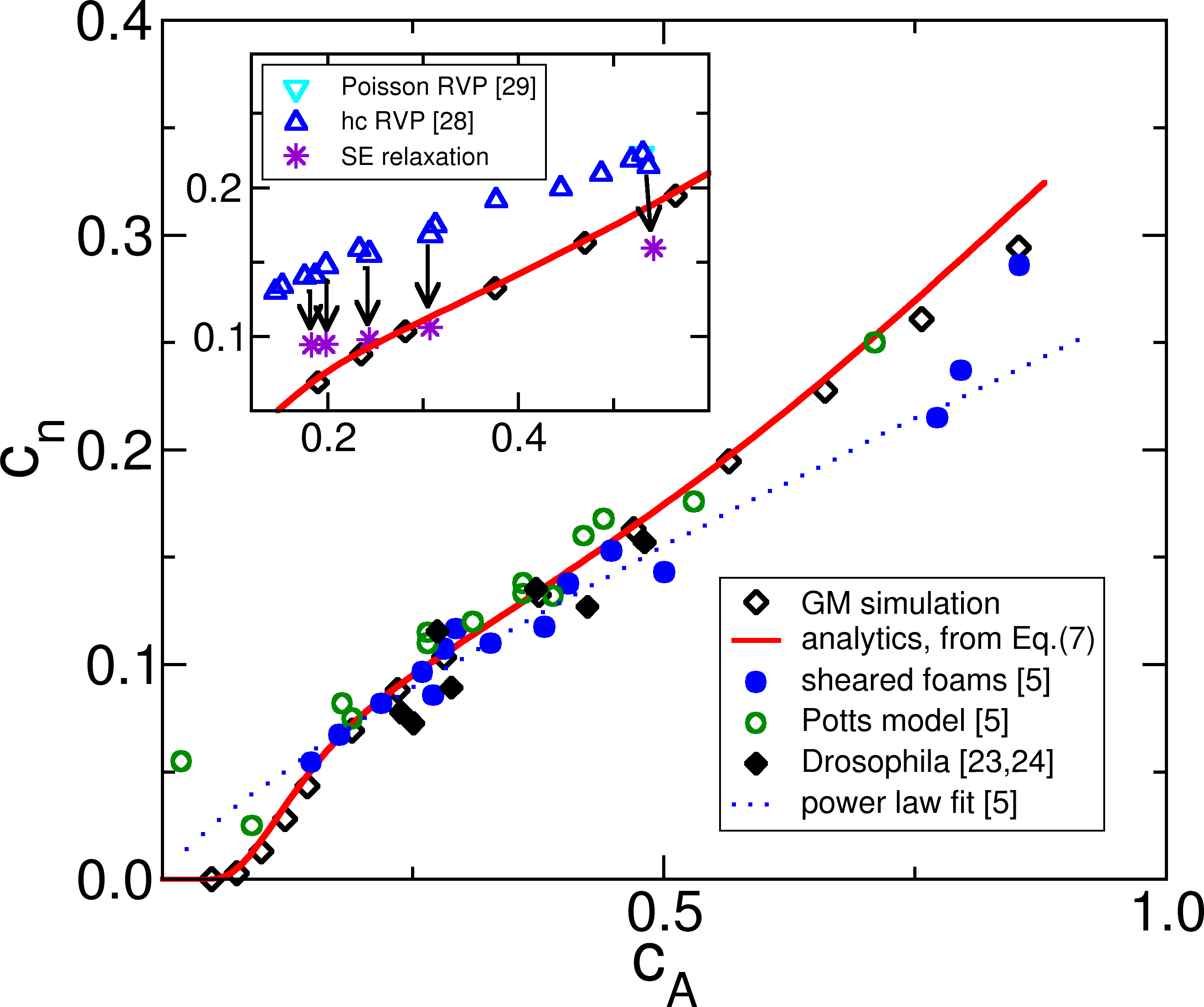
Figure 1: Dependence of topological disorder $c_{n}$ on size disorder $c_{A}$ in random cellular networks. The analytical theory (solid line) and GM simulations (open diamonds) are in excellent agreement with each other and empirical data (closed symbols: experiments, open symbols: simulations). The inset show that RVP and hard-core (hc) RVP tilings do not obey this correlation (triangles), but when these structures undergo energy minimization in Surface Evolver (arrows), they approach the GM prediction (stars). The dotted line is the power-law fit of Quilliet et al. (2008).

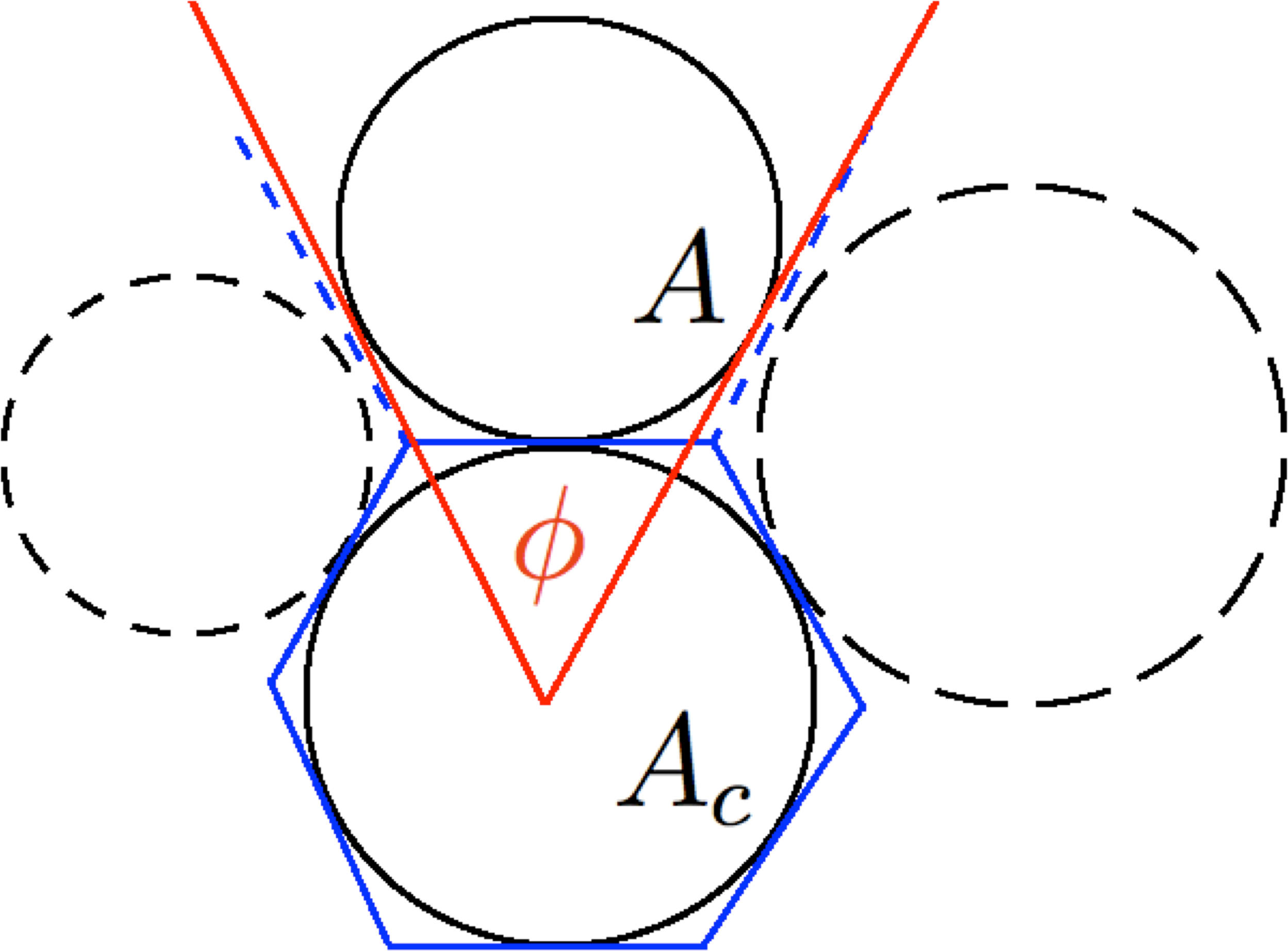
Figure 2: Local disc packing in the modified 2D granocentric model: a disc of area $A_{c}$ is surrounded by discs of area $A$ subtending angles $\phi$. The discs serve as templates for polygonal cell construction.

Very recently, a local model for 3D systems has been developed incorporating a simple connection between size and neighbor topology. The granocentric model Clusel et al. ; Corwin et al. (2010) (GM) of Brujić et al. analyzes the solid angles taken up by spheres neighboring a central sphere and, given the size distribution of spheres, numerically predicts probabilities of numbers of neighbors $n$ and touching neighbors $z$. To self-consistently reproduce the observed $n$, the model must modify the total available solid angle around a sphere ($4\pi$) to $4\pi-\epsilon_{3}$, where empirically $\epsilon_{3}\approx 0.32\pi$Corwin et al. (2010). We extend the GM to the 2D case and show that, under certain general approximations, its formalism becomes analytically solvable without free parameters.

We consider 2D polydisperse hard discs with area probability distribution $P(A)$, normalized to the mean $\bar{A}=1$. As any packing can be converted to a polygonal tiling by constructing cells around the discs (Fig. 2), this also describes a tiling with a distribution $P_{p}(A)$. With our main focus on such tilings, we will not model touching neighbors, but only the probability $P_{n}$ of having $n$ general neighbors. A central disc of area $A_{c}$ is then surrounded by $n$ discs of area $A$ (Fig. 2), where every disc subtends an angle

$$\phi=g(A)=2\arcsin\left(1/(1+\sqrt{A_{c}/A})\right)$$ (1)

around the central disc, resulting in the probability distribution of angles $f_{c}(\phi)=P(A(\phi))(dg^{-1}/d\phi).$ Following Corwin et al. (2010), we can now compute the conditional probability $P(n|A_{c})$ and the neighbor probability $P_{n}$ through

$$P(n|A_{c}) = \int_{0}^{\phi_{max}}R_{c,n}(\phi)F(\phi_{max}-\phi)d\phi\,,$$

$$P_{n} = \int P(n|A_{c})P(A_{c})dA_{c}\,.$$ (2)

Here, $R_{c,n}(\phi)$ is the probability of the sum of $n$ angles from (1) reaching $\phi$ and $F(\phi_{max}-\phi)\equiv\int_{\phi_{max}-\phi}^{\infty}f_{c}(\phi)d\phi$ expresses the probability of the $(n+1)^{th}$ angle exceeding $\phi_{max}$. The maximum angle $\phi_{max}$ available for neighboring discs is again $\not=2\pi$ because of steric effects. But as Euler’s theorem Grunbaum and Shephard (1987) demands $\bar{n}=6$ in 2D (for generic three-fold coordinated edges between neighbors), $\phi_{max}=2\pi+\epsilon$ can be determined analytically: To leading order in $c_{A}\ll 1$, after fitting 5 (touching) neighbors around a disc, there will be a $50\%$ chance of being able to fit a sixth neighbor, i.e., for the unmodified $\phi_{max}=2\pi$ we obtain $\bar{n}=5.5$. To fit, on average, 0.5 additional neighbors, we need to supply the additional average angle subtended by 1/2 disc, i.e., $\epsilon=\pi/6$ and $\phi_{max}=13\pi/6$. Higher-order terms in $c_{A}$ can be obtained, but we will show that this argument is sufficient in the entire range of relevant $c_{A}$.

Eq. (2) can be evaluated numerically for realistic size and angle distributions. In cellular materials, these are usually gamma or shifted-gamma distributions Kumar and Kumaran (2005a); Lemaître et al. (1993); Jorjadze et al. (2011); Weibull Wyn, A. et al. (2008) and other unimodal distributions have also been used. We employ a gamma distribution fit to $f_{c}(\phi)$ to evaluate (2) numerically; the results are indicated by the label ”GM simulations” in subsequent plots. We stress that we have also tried Weibull and other fits with the same mean and variance, and obtained almost indistinguishable results sup .

Beyond numerical evaluation, however, we can derive analytical results by instead choosing a normal distribution as fit to $f_{c}$, again preserving the first and second moments. The quality of this approximation can be assessed rigorously through an Edgeworth expansion Wallace (1958) and confirmed numerically. As detailed in the Supplemental Material, the approximation is found to give very accurate results independent of the exact distribution function. We stress that our analytics derive from the single parameter $c_{A}$ only, with $c_{A}\mbox{\ \raisebox{-3.87495pt}{$\stackrel{{\scriptstyle\textstyle<}}{{\sim}}$}\ }0.5$ for the vast majority of systems encountered experimentally or theoretically and $c_{A}\mbox{\ \raisebox{-3.87495pt}{$\stackrel{{\scriptstyle\textstyle<}}{{\sim}}$}\ }0.85$ for all instances we could find; thus, expansions in $c_{A}$ as a small parameter are possible. Expanding $P(A)$ around $\bar{A}=1$, the coefficient of variation of $f_{c}(\phi)$ is obtained to ${\cal O}(c_{A}^{2})$ from (1) as

$$c_{\phi}=c_{A}/\left([g^{-1}]^{\prime}[g(1)]g(1)\right)\,.$$ (3)

With Gaussian $f_{c}$, $R_{c,n}$ is Gaussian as well, with $n$-fold mean and variance, while $F$ is an error function. Then, $P(n|A_{c})$ in (2) is obtained using $\int_{-\infty}^{\infty}\exp(-(Ax+B)^{2}){\rm erf}(Cx+D)dx=(\sqrt{\pi}/A){\rm erf}((AD-BC)/\sqrt{A^{2}+C^{2}})$ Simon and Divsalar (1998), yielding $P(n|A_{c})=\Phi_{n+1}(c_{A},A_{c})-\Phi_{n}(c_{A},A_{c})$, where

$$\Phi_{n}(c_{A},A_{c})={1\over 2}{\rm erf}\left({n\bar{\phi}(A_{c})-\phi_{max}\over\sqrt{2n}\sigma_{\phi}(c_{A},A_{c})}\right)\,,$$ (4)

with $\bar{\phi}(A_{c})=2\arcsin(1/(1+\sqrt{A_{c}}))$ and, to leading order in $c_{A}$, the variance $\sigma^{2}_{\phi}=c_{A}^{2}s/((1+s)^{2}(2+s))$, with $s\equiv\sqrt{A_{c}}$.

Linearizing the argument of this error function around its root in $A_{c}$, and again making use of a consistent Gaussian approximation with width $c_{A}$ for $P(A_{c})$, we obtain a second integral of the same type, yielding, after further expansion for small $c_{A}$, the explicit prediction for neighbor probability $P_{n}=\Psi_{n+1}(c_{A})-\Psi_{n}(c_{A})$, with

$$\Psi_{n}(c_{A})\!=\!{1\over 2}{\rm erf}\left({\sqrt{2n}\left(1-(2-c_{A}^{2}/8)\Sigma\right)\over c_{A}\!\!\left(\left(1-\Sigma\right)^{2}\!\!+\!n(1-c_{A}^{2}/8)\Sigma^{2}\right)^{{1\over 2}}}\right)\!,$$ (5)

where $\Sigma\equiv\sin(13\pi/12n)=\sin(\phi_{max}/2n)$ sup .

We first interpret these results for discs (without constructing polygonal domains). Plotting the predicted $P_{n}(c_{A})$, we observe a pronounced plateau of hexagonal order in the near-monodisperse case of small $c_{A}$ (Fig. 3), so that $P_{6}\approx 1$ for $c_{A}\leq c_{A,crit}$. This effect of crystallization is well known in simulations of hard-disc packings Ito (1996); Donev et al. (2004); Santen and Krauth (2000), where a certain amount of polydispersity Sadr-Lahijany et al. (1997); Santen and Krauth (2001) or bidispersity Donev et al. (2006) is necessary to achieve a random structure. The critical $c_{A}$ (terminal polydispersity), below which crystallization into ordered domains occurs, has been empirically determined to be $c_{A,crit}\mbox{\ \raisebox{-3.87495pt}{$\stackrel{{\scriptstyle\textstyle<}}{{\sim}}$}\ }0.1$ Ito (1996); Sadr-Lahijany et al. (1997); Santen and Krauth (2001). In the limit $c_{A}\to 0$, (5) can be further expanded around $n=13/2$, which yields, to excellent accuracy, a compact formula for the fraction of hexagonally coordinated discs,

$$P_{6}={\rm erf}\left(\gamma/c_{A}\right)\,,$$ (6)

where $\gamma^{2}\equiv 2\pi^{2}/585$. Figure 3 shows that the approximations (5),(6) capture both the numerical results (GM) and the empirically observed feature of crystallization (Eq. (6) is indistinguishable from (5) with $n=6$). The point of largest curvature of $P_{6}(c_{A})$, where the crystallization plateau begins, is the critical polydispersity $c_{A,crit}=\gamma/\sqrt{3}\approx 0.106$, in very good agreement with empirical values of terminal polydispersity.

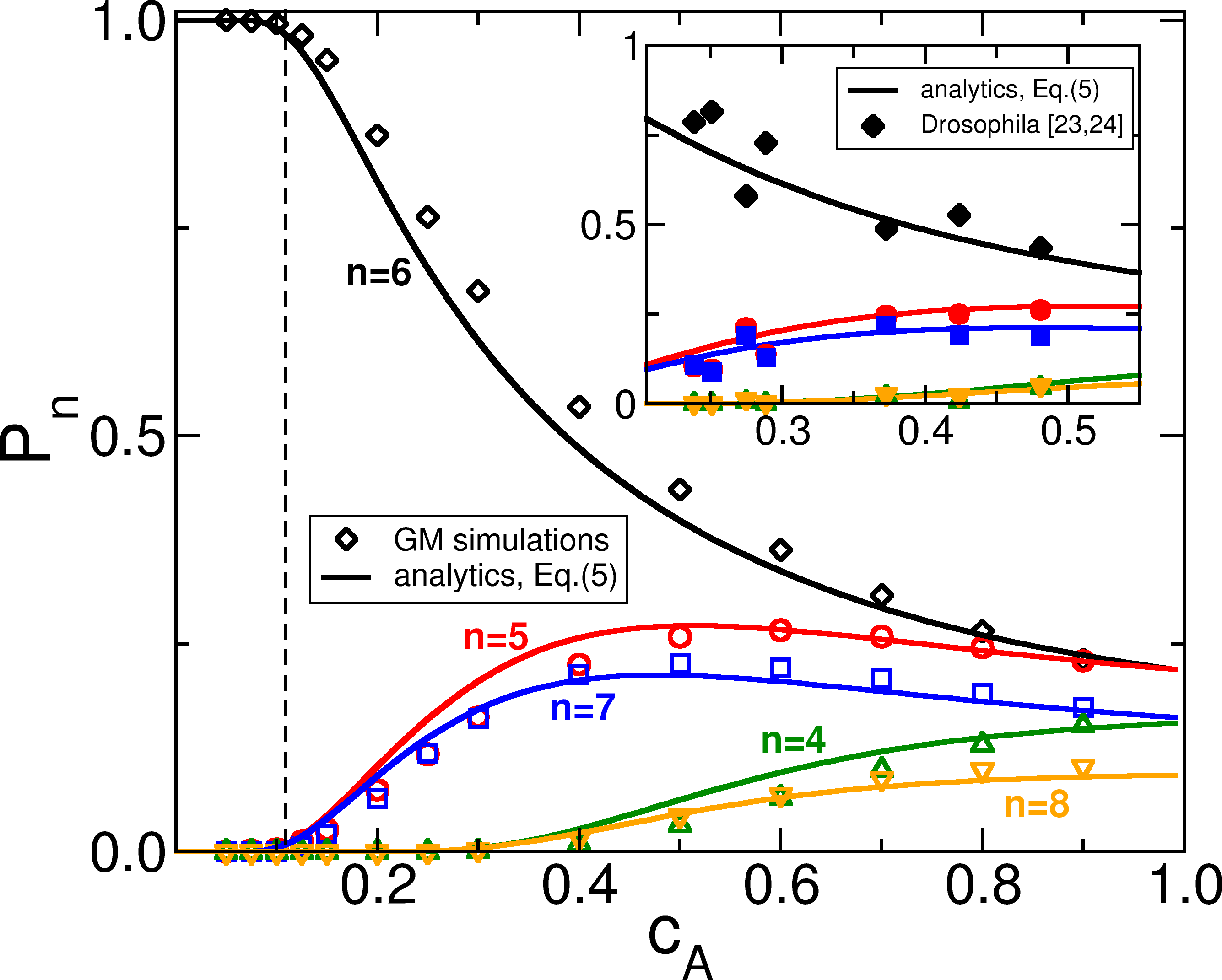
Figure 3: Neighbor probabilities $P_{4}$ (triangles up), $P_{5}$ (circles), $P_{6}$ (diamonds), $P_{7}$ (squares), $P_{8}$ (triangles down) of discs in the GM simulations. Solid lines are analytical approximations. The plateau of $P_{6}\approx 1$ quantifies the range of crystallization near monodispersity with $c_{A,crit}=\gamma/\sqrt{3}$ (dashed vertical line). The inset illustrates that the disc $P_{n}$ are good predictors for numbers of cellular neighbors in random tilings, here for Drosophila wing tissue cells Classen et al. (2005); Gibson et al. (2006).

The crystallization threshold divides the regime of nearly-monodisperse objects (where additional orientational disorder, absent from the model, could maintain randomness, e.g. in monodisperse cellular tilings) from that of polydisperse objects (where size disorder overwhelms positional disorder Corwin et al. (2010)). In the latter regime, polygonal cells constructed around the discs should be characterized by the same relations as the discs themselves. As an example, the predicted $P_{n}$ match experimental data Classen et al. (2005); Miklius, M.P. and Hilgenfeldt, S. (2011) for neighbor probabilities in cellular tissues very well, see inset of Fig. 3 (note that topological asymmetry such as $P_{5}\not=P_{7}$ is obtained without skewness information from $P(A)$). In the following, we compare the results of the GM and analytical calculations to empirical size-toplogy correlation data from cellular systems. In order to translate the disc areas into polygonal areas, we simply assume that a disc of area $A$ with $n$ neighbors is inscribed into a regular $n$-gon (with area $A_{p}=(n/\pi)\tan(\pi/n)A$), and re-normalize the resulting areas. All area-related quantities in Figs. 1 and 4 thus refer to polygonal areas. While the assumption of regular polygons misses some of the disorder in the system, for cellular systems with domain energy the difference of domain areas from those of regular polygons is typically very small (cf. e.g. Graner et al. (2000)).

The expansion that yields (6) also gives the variance $\mu_{2,n}$ of $P_{n}$, and thus $c_{n}=\mu_{2,n}^{1/2}/\bar{n}$. We find

$$\mu_{2,n}=\sum_{k=1}^{\infty}(2k-1){\rm erfc}((2k-1){\gamma\over 2c_{A}})\,,$$ (7)

which converges rapidly (even for $c_{A}\to 1$, truncating the series after the third term is very accurate). Figure 1 shows the resulting analytical $c_{n}(c_{A})$, together with numerical results and various empirical data points. Also shown is the power-law fit of Quilliet et al. (2008). We see that, for $c_{A}>c_{A,crit}$, the agreement is excellent for a large variety of systems. However, simulations of random Voronoi polygon (RVP) tilings Brakke (2005); Zhu (2001) significantly disagree with the GM theory and appear to lie on a separate line in $c_{n}-c_{A}$ space (inset of Fig. 1).

We suggest that this is caused by the RVP domains’ lack of a compact shape, which in turn is due to the absence of an interfacial energy functional. Almost all physical cellular systems, by contrast, exhibit an energy penalty for domain boundaries. We tested this hypothesis by digitizing some of the RVP structures from Zhu (2001), using them as initial conditions for an energy minimization of the structure (under constant domain areas) using Surface Evolver Brakke (1992) (SE) with a uniform interfacial energy density. As the inset of Fig. 1 shows, the topological disorder $c_{n}$ indeed diminishes during this process (due to T1 transitions Weaire and Hutzler (2000)) until the systems approach the observed general $c_{n}-c_{A}$ correlation.

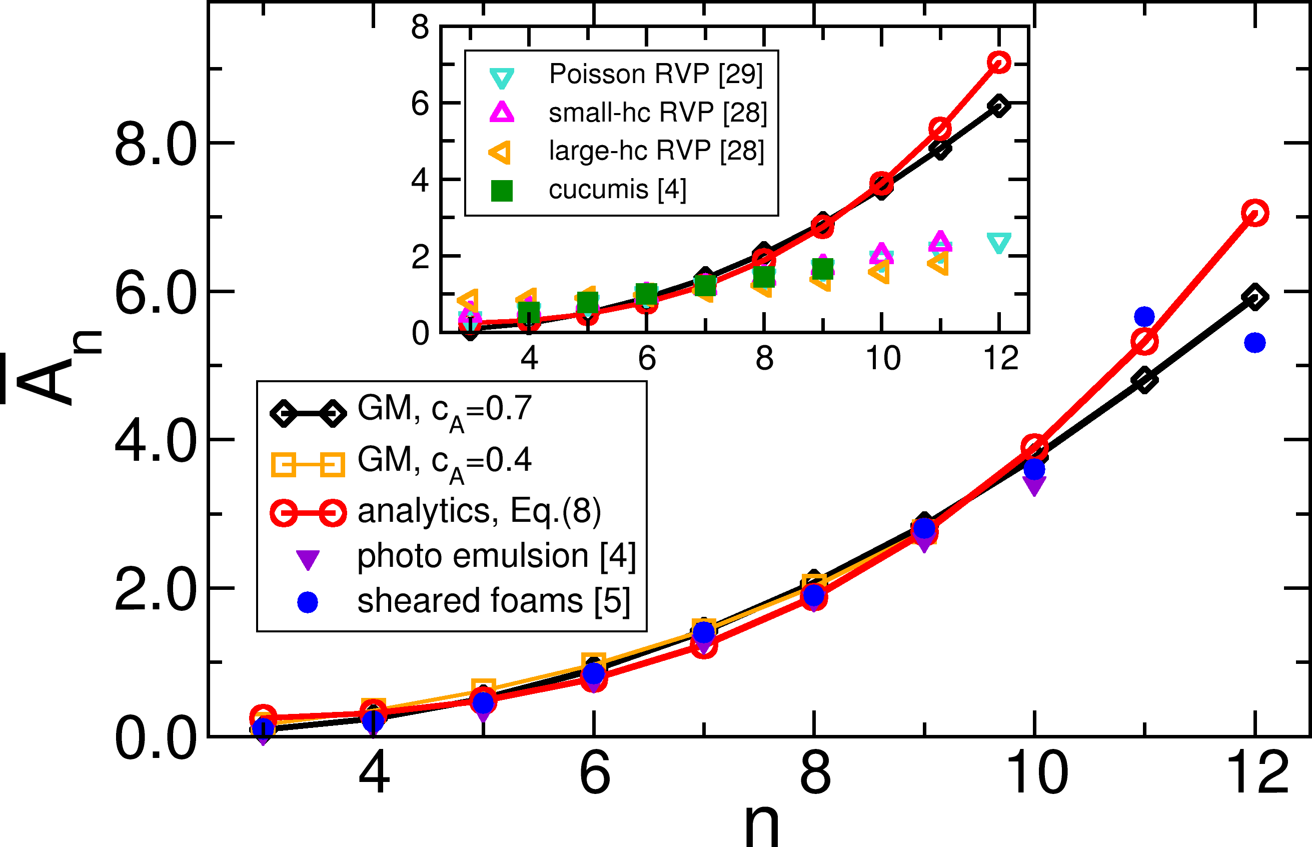
Figure 4: The dependence of $\bar{A}_{n}$ on $n$ is nonlinear in disc and most cellular systems. The analytical prediction for this nonlinear Lewis’ law agrees well with simulations and experimental data up to $n\approx 10$. Random Voronoi polyhedra with Zhu (2001) or without hard cores Brakke (2005) do not follow this prediction (inset). Lewis’ data on cucumber tissue Lewis (1931) also appears to be in this class.

The Lewis law correlation can be derived within the GM by computing $\bar{A}_{n}=\int A_{c}P(n|A_{c})P(A_{c})dA_{c}/P_{n}$, using the same algorithm as above, including expansions in small $c_{A}$ and around $n=13/2$ sup . Interestingly, the $c_{A}$-dependences cancel to leading order, giving the $c_{A}$-independent approximation

$$\bar{A}_{n}=\exp\left({2n(1-\Sigma)\Sigma\over(1-\Sigma)^{2}+n\Sigma^{2}}\right)\,.$$ (8)

This is in agreement with our numerical results that show $\bar{A}_{n}$ to be insensitive to $c_{A}$, as well as experimental and other empirical data Quilliet et al. (2008); Lewis (1931) that confirm this distinctly nonlinear form of Lewis’ law (8), see Fig. 4. The systems for which the $c_{n}-c_{A}$ correlation fails (Fig. 1) display a linear Lewis’ law, clearly disagreeing with the GM theory (inset of Fig. 4) and again suggesting two distinct classes of systems distinguishable by compactness of the individual domains. Surface Evolver relaxation of the RVP structures cannot restore the nonlinear Lewis’ law, because larger areas are not part of the area distribution, which is not changed by SE.

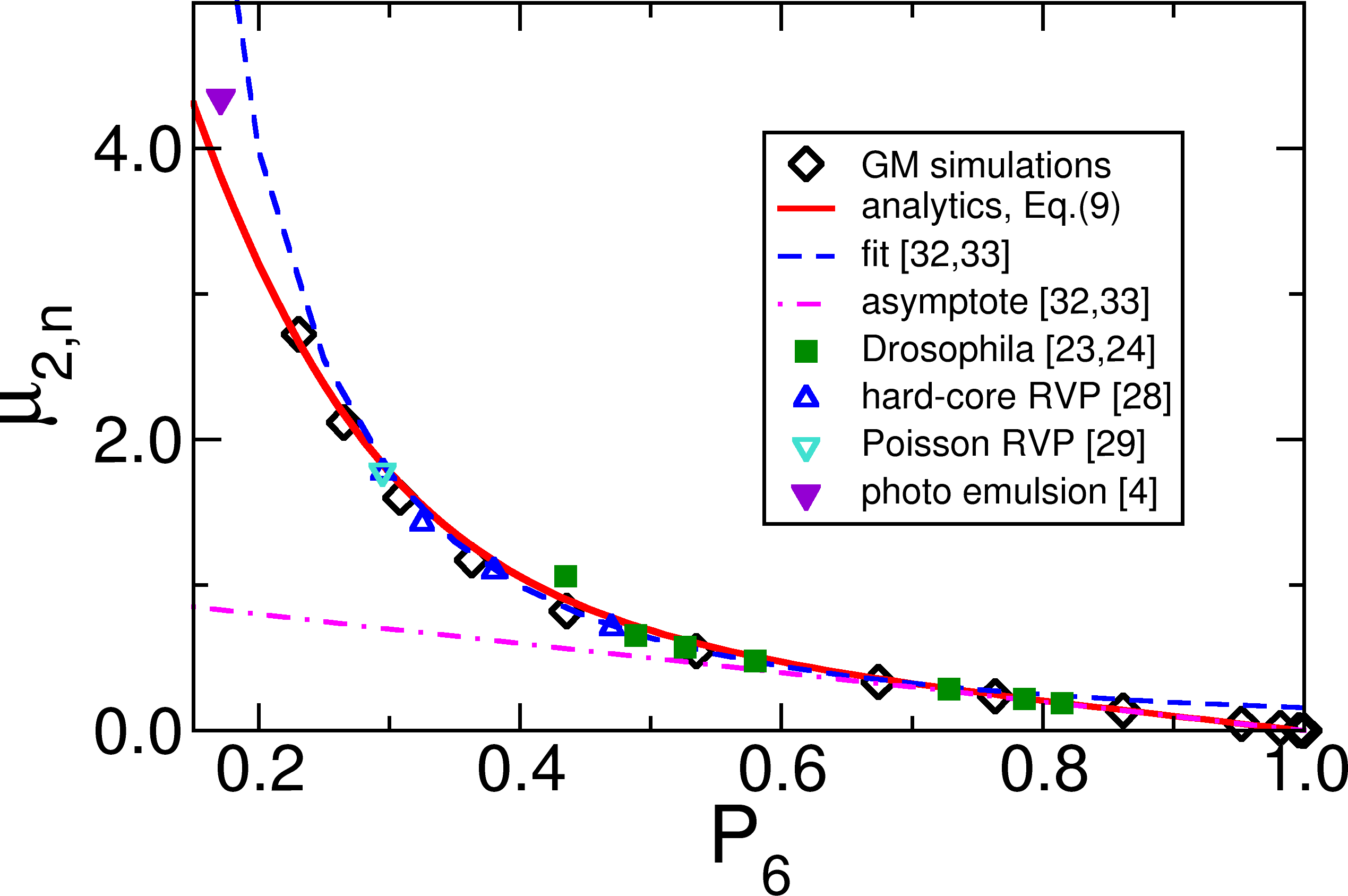
Figure 5: Lemaître’s law, a robust correlation between $P_{6}$ and the toplogical variance $\mu_{2,n}$. The analytical theory from the first three terms of (9) is given as solid line, confirmed to great accuracy by many empirical data points and GM simulations (symbols).

A relation between $P_{6}$ and $\mu_{2,n}$ has been reported as Lemaître’s law J. Lemaître and Bidcau (1991); Lemaître et al. (1993), with an empirical two-part fit suggested by LeCaër and Delannay (1993); Rivier et al. (1995). The present formalism again provides concise formulae: from (6), we obtain the leading-order inversion $\gamma/c_{A}\approx\sqrt{\pi}P_{6}$, which combined with (7) yields

$$\mu_{2,n}(P_{6})=\sum_{k=1}^{\infty}(2k-1){\rm erfc}\left((2k-1){\sqrt{\pi}\over 2}P_{6}\right)\,.$$ (9)

As $P_{6}\to 1$, this immediately reduces to $\mu_{2,n}=1-P_{6}$, in agreement with LeCaër and Delannay (1993); Rivier et al. (1995). As Fig. 5 shows, (9) is a uniformly valid approximation that captures both empirical fits in the reported range of $P_{6}\mbox{\ \raisebox{-3.87495pt}{$\stackrel{{\scriptstyle\textstyle>}}{{\sim}}$}\ }0.3$ LeCaër and Delannay (1993); Rivier et al. (1995). Even though (9) relates two topological quantities, it could only be derived through the area distribution. Lemaître’s law holds very robustly, being valid for all experimental, simulation, and analytical data. In this sense, all of the analytical information about topological disorder in these systems is contained in $P_{6}$.

We have shown that a purely local formalism, a generalization of the granocentric model in two dimensions, yields accurate and general predictions for size-topology correlations in cellular matter, using only the coefficient of variation of the unimodal area distribution. Further generalizations are feasible in future work, including neighbor correlations (Aboav-Weaire law) or higher moments of the distributions (e.g. to obtain $C_{k}$ measures Kumar and Kumaran (2005b)). As a leading-order theory, the present formalism does surprisingly well and puts a number of empirical relations on a firm footing.

Acknowledgments: The authors thank J. Brujić and E.  Vanden-Eijnden for a frank exchange of ideas and results, and invaluable advice and clarifications about the GM.

References

- Thompson (1942) D. Thompson, On Growth and Form (Cambridge University Press, 1942).
- Lecuit and Lenne (2007) T. Lecuit and P. F. Lenne, Nature Reviews Molecular Cell Biologyl 8, 633 (2007).
- Lewis (1928) F. Lewis, The Anatomical Record 38, 341 (1928).
- Lewis (1931) F. Lewis, The Anatomical Record 50, 235 (1931).
- Quilliet et al. (2008) C. Quilliet, S. A. Talebi, D. Rabaud, S. C. J. Käfer, and F. Graner, Phil. Mag. Lett. 88, 651 (2008).
- Glazier et al. (1987) J. A. Glazier, S. P. Gross, and J. Stavans, Phys. Rev. A 36, 306 (1987).
- Lemaître et al. (1993) J. Lemaître, A. Gervois, J. P. Troadec, N. Rivier, M. Ammi, L. Oger, and D. Bideau, Philosophical Magazine Part B 67, 347 (1993).
- (8) M. Clusel, E. I. Corwin, A. O. N. Siemens, and J. Brujic, Nature 460, 611.
- Corwin et al. (2010) E. I. Corwin, M. Clusel, A. O. N. Siemens, and J. Brujic, Soft Matter 6, 2949 (2010).
- Grunbaum and Shephard (1987) B. Grunbaum and G. C. Shephard, Tilings and Patterns (W. H. Freeman and Company, New York, 1987).
- Kumar and Kumaran (2005a) V. S. Kumar and V. Kumaran, J. Chem. Phys. 123, 114501 (2005a).
- Jorjadze et al. (2011) I. Jorjadze, L.-L. Pontani, K. A. Newhall, and J. Brujić, Proceedings of the National Academy of Sciences 108, 4286 (2011).
- Wyn, A. et al. (2008) Wyn, A., Davies, I. T., and Cox, S. J., Eur. Phys. J. E 26 (2008).
- (14) See the Supplemental Material for more details.
- Wallace (1958) D. L. Wallace, The Annals of Mathematical Statistics 29, pp. 635 (1958).
- Simon and Divsalar (1998) M. K. Simon and D. Divsalar, IEEE Trans. Comm. 46, 200 (1998).
- Ito (1996) N. Ito, Int. J. Mod. Phys. C 7, 275 (1996).
- Donev et al. (2004) A. Donev, S. Torquato, F. H. Stillinger, and R. Connelly, J. Appl. Phys. 95, 989 (2004).
- Santen and Krauth (2000) L. Santen and W. Krauth, Nature 405, 550 (2000).
- Sadr-Lahijany et al. (1997) M. R. Sadr-Lahijany, P. Ray, and H. E. Stanley, Phys. Rev. Lett. 79, 3206 (1997).
- Santen and Krauth (2001) L. Santen and W. Krauth, (2001).
- Donev et al. (2006) A. Donev, F. H. Stillinger, and S. Torquato, Phys. Rev. Lett. 96, 225502 (2006).
- Classen et al. (2005) A. Classen, K. Anderson, E. Marois, and S. Eaton, Developmental Cell 9, 805 (2005).
- Gibson et al. (2006) M. Gibson, A. Patel, R. Nagpal, and N. Perrimon, Nature 442, 1038 (2006).
- Miklius, M.P. and Hilgenfeldt, S. (2011) Miklius, M.P. and Hilgenfeldt, S., Eur. Phys. J. E 34, 50 (2011).
- Graner et al. (2000) F. Graner, Y. Jiang, E. Janiaud, and C. Flament, Phys. Rev. E. 63, 114021 (2000).
- Brakke (2005) K. Brakke, “200,000,000 random voronoi polygons,” (2005).
- Zhu (2001) H. Zhu, Philosophical Magazine A 81, 2765 (1 December 2001).
- Brakke (1992) K. Brakke, Experimental Mathematics 1, 141 (1992).
- Weaire and Hutzler (2000) D. Weaire and S. Hutzler, The Physics of Foams (Oxford University Press, Oxford, 2000).
- J. Lemaître and Bidcau (1991) A. G. J. Lemaître, J.-P. Troadec and D. Bidcau, Europhysics Leters 14, 77 (1991).
- LeCaër and Delannay (1993) G. LeCaër and R. Delannay, J. Phys. A 26, 3931 (1993).
- Rivier et al. (1995) N. Rivier, G. Schliecker, and B. Dubertret, Acta Biotheoretica 43, 403 (1995).
- Kumar and Kumaran (2005b) V. S. Kumar and V. Kumaran, J. Chem. Phys. 123, 074502 (2005b).