Isostaticity, auxetic response, surface modes, and conformal invariance in twisted kagome lattices

Abstract

Model lattices consisting of balls connected by central-force springs provide much of our understanding of mechanical response and phonon structure of real materials. Their stability depends critically on their coordination number $z$. $d$-dimensional lattices with $z=2d$ are at the threshold of mechanical stability and are isostatic. Lattices with $z<2d$ exhibit zero-frequency “floppy” modes that provide avenues for lattice collapse. The physics of systems as diverse as architectural structures, network glasses, randomly packed spheres, and biopolymer networks is strongly influenced by a nearby isostatic lattice. We explore elasticity and phonons of a special class of two-dimensional isostatic lattices constructed by distorting the kagome lattice. We show that the phonon structure of these lattices, characterized by vanishing bulk moduli and thus negative Poisson ratios and auxetic elasticity, depends sensitively on boundary conditions and on the nature of the kagome distortions. We construct lattices that under free boundary conditions exhibit surface floppy modes only or a combination of both surface and bulk floppy modes; and we show that bulk floppy modes present under free boundary conditions are also present under periodic boundary conditions but that surface modes are not. In the the long-wavelength limit, the elastic theory of all these lattices is a conformally invariant field theory with holographic properties, and the surface waves are Rayleigh waves. We discuss our results in relation to recent work on jammed systems. Our results highlight the importance of network architecture in determining floppy-mode structure.

I Introduction

Networks of balls and springs or frames of nodes connected by compressible struts provide realistic models for physical systems from bridges to condensed solids. Their elastic properties depend on their coordination number $z$ – the average number of nodes each node is connected to. If $z$ is large enough, the networks are elastic solids whose long-wavelength mechanical properties are described by a continuum elastic energy with non-vanishing elastic moduli. If $z$ is small enough, the networks have deformation modes of zero energy – they are floppy. As $z$ is increased from the floppy side, a critical value, $z_{c}$, is reached at which springs provide just enough constraints that the system has no zero-energy “floppy” modes Thorpe1983 (or mechanisms Calladine1978 in the engineering literature), and the system is isostatic. The phenomenon of rigidity percolation FengSen1984 ; JacobsTho1995 whereby a sample spanning rigid cluster develops upon the addition of springs is one version of this floppy-to-rigid transition. The coordination numbers of whole classes of systems, including engineering structures Heyman1999 ; Kassimali2005 (bridges and buildings), randomly packed spheres near jamming LiuNag1998 ; LiuNag2010a ; LiuNag2010b ; TorquatoSti2010 , network glasses Phillips1981 ; Thorpe1983 , cristobalites HammondsWin1996 , zeolites Zeolitereview ; SartbaevaTho2006 , and biopolymer networks WilhelmFre2003 ; HeussingerFrey2006 ; HuismanLub2011 ; BroederszMac2011 are close enough to $z_{c}$ that their elasticity and mode structure is strongly influenced by those of the isostatic lattice.

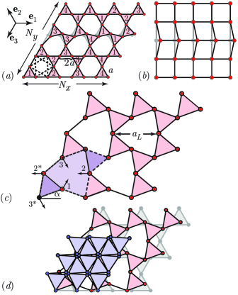
Figure 1: (a) Section of a kagome lattice with $N_{x}=N_{y}=4$ and $N_{c}=N_{x}N_{y}$ three-site unit cells. Nearest-neighbor bonds, occupied by harmonic springs, are of length $a$. The rotated row (second row from the top) represents a floppy mode. Next-nearest neighbor bonds are shown as dotted lines in the lower left hexagon. The vectors $\mathbf{e}_{1}$, $\mathbf{e}_{2}$, and $\mathbf{e}_{3}$ indicate symmetry directions of the lattice. The numbers in the triangles indicate those that twist together under PBCs in zero modes along the three symmetry direction. Note that there are only $4$ of these modes. (b) Section of a square lattice depicting a floppy mode in which all sites along a line are displaced uniformly. (c) Twisted kagome lattice, with lattice constant $a_{L}=2a\cos\alpha$, derived from the undistorted lattice by rigidly rotating triangles through an angle $\alpha$. A unit cell, bounded by dashed lines, is shown in violet. Arrows depict site displacements for the zone-center, i.e., zero wavenumber, $\phi$ mode which has zero (nonzero) frequency under free (periodic) boundary conditions. Sites $1$, $2$, and $3$ undergo no collective rotation about their center of mass whereas sites $1$, $2^{*}$, and $3^{*}$ do. (d) Superposed snapshots of the twisted lattice showing decreasing areas with increasing $\alpha$.

Though the isostatic point always separates rigid from floppy behavior, the properties of isostatic lattices are not universal; rather they depend on lattice architecture. Here we explore the the unusual properties of a particular class of periodic isostatic lattices derived from the two-dimensional kagome lattice by rigidly rotating triangles through an angle $\alpha$ without changing bond lengths as shown in Fig. 1. The bulk modulus $B$ of these lattices is rigorously zero for all $\alpha\neq 0$. As a result, their Poisson ratio acquires its limit value of $-1$; when stretched in one direction, they expand by an equal amount in the orthogonal direction: they are maximally auxetic Lakes1987 ; EvansRog1991 ; LakesChe1991 ; GreavesRou2011 . These modes represent collapse pathways HutchinsonFle2006 ; KapkoGue2009 of the kagome lattice. Modes of isostatic systems are generally very sensitive to boundary conditions Wyartwit2005b ; Wyart2005 ; TorquatoSti2001 , but the degree of sensitivity depends on the details of lattice structure. For reasons we will discuss more fully below, modes of the square lattice, which is isostatic, are in fact insensitive to changes from free boundary conditions (FBCs) to periodic boundary conditions (PBCs), whereas those of the undistorted kagome lattice are only mildly so. The modes of both, however, change significantly when rigid boundary conditions (RGBs) are applied. We show here that in all families of the twisted kagome lattice, modes depend sensitively on whether FBCs, PCBs or RGBs are applied: finite lattices with free boundaries have floppy surface modes that are not present in their periodic or rigid spectrum or in that of finite undistorted kagome lattices. In the long wavelength limit, the surface floppy modes, which are present in any $2d$ material with $B=0$, reduce to surface Rayleigh waves Landau-elasticity described by a conformally invariant energy whose analytic eigenfunctions are fully determined by boundary conditions. At shorter wavelengths, the surface waves become sensitive to lattice structure and remain confined to within a distance of the surface that diverges as the undistorted kagome lattice is approached. In the simplest twisted kagome lattice, all floppy modes are surface modes, but in more complicated lattices, including ones with uniaxial symmetry, we construct, there are both surface and bulk floppy modes.

Arguments due to J.C. Maxwell Maxwell1864 provide a criterion for network stability: networks in $d$ dimensions consisting of $N$ nodes, each connected with central-force springs to an average of $z$ neighbors, have $N_{0}=dN-\frac{1}{2}zN$ zero-energy modes when $z<2d$ (in the absence of redundant bonds - see below). Of these a number, $N_{\rm tr}$, which depends on boundary conditions, are trivial rigid translations and rotations, and the and the remainder are floppy modes of internal structural rearrangement. Under FBCs an PBCs, $N_{\rm tr}$ equals $d(d+1)/2$ and $d$, respectively. With increasing $z$, mechanical stability is reached at the isostatic point at which $N_{0}=N_{\rm tr}$. The Maxwell argument is a global one; it does not provide information about the nature of the floppy modes and does not distinguish between bulk or surface modes.

II Kagome zero modes and elasticity

The kagome lattice of central force springs shown in Fig. 1(a) is one of many locally isostatic lattices, including the familiar square lattice lattice in two dimensions [Fig. 1(b)] and the cubic and pyrochlore lattices in three dimensions, with exactly $z=2d$ nearest-neighbor ($NN$) bonds connected to each site not at a boundary. Under PBCs, there are no boundaries, and every site has exactly $2d$ neighbors. Finite, $N$-site sections of these lattices have surface sites with fewer than $2d$ neighbors and of order $\sqrt{N}$ zero modes. The free kagome lattice with $N_{x}$ and $N_{y}$ unit cells along its sides [Fig. 1(a)] has $N=3N_{x}N_{y}$ sites, $N_{B}=6N_{x}N_{y}-2(N_{x}+N_{y})+1$ bonds, and $N_{0}=2(N_{x}+N_{y})-1$ zero modes, all but three of which are floppy modes. These modes, depicted in Fig. 1(a), consist of coordinated counter rotations of pairs of triangles along the symmetry axes $\mathbf{e}_{1}$, $\mathbf{e}_{2}$ and $\mathbf{e}_{3}$ of the lattice. There are $N_{x}$ modes associated with lines parallel to $\mathbf{e}_{1}$, $N_{y}$ associated with lines parallel to $\mathbf{e}_{3}$, and $N_{x}+N_{y}-1$ modes associated with lines parallel to $\mathbf{e}_{2}$.

In spite of the large number of floppy modes in the kagome lattice, its longitudinal and shear Lamé coefficients, $\lambda$ and $\mu$, and its Bulk modulus $B=\lambda+\mu$ are nonzero and proportional to the nearest neighbor ($NN$) spring constant $k$: $\lambda=\mu=\sqrt{3}k/8$, and $B=\lambda+\mu=\sqrt{3}k/4$. The zero modes of this lattice can be used to generate an infinite number of distorted lattices with unstretched springs and thus zero energy KapkoGue2009 ; SouslovLub2011 . We consider only periodic lattices, the simplest of which are the twisted kagome lattices obtained by rotating triangles of the kagome unit cell through an angle $\alpha$ as shown in Figs. 1(c) and (d) GrimaEva2005 ; KapkoGue2009 . These lattices have $C_{3v}$ rather than $C_{6v}$ symmetry and, like the undistorted kagome lattice, three sites per unit cell. As Fig. 1(d) shows, the lattice constant of these lattices is $a_{L}=2a\cos\alpha$, and their area $A_{\alpha}$ decreases as $\cos^{2}\alpha$ as $\alpha$ increases. The maximum value that $\alpha$ can achieve without bond crossings is $\pi/3$ so that the maximum relative area change is $A_{\pi/3}/A_{0}=1/4$. Since all springs maintain their rest length, there is no energy cost for changing $\alpha$, and as a result, $B$ is zero for every $\alpha\neq 0$, whereas the shear modulus $\mu=\sqrt{3}k/8$ remains nonzero and unchanged. Thus, the Poisson ratio $\sigma=(B-\mu)/(B+\mu)$ attains its smallest possible value of $-1$. For any $\alpha\neq 0$, the addition of next-nearest-neighbor ($NNN$) springs, with spring constant $k^{\prime}$ (or of bending forces between springs) stabilizes zero-frequency modes and increases $B$ and $\sigma$. Nevertheless, for sufficiently small $k^{\prime}$, $\sigma$ remains negative. Figure 2 shows the region in the $k^{\prime}-\alpha$ plane with negative $\sigma$.

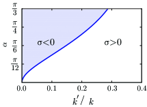
Figure 2: phase diagram in the $\alpha-k^{\prime}$ plane showing region with negative Poisson ratio $\sigma$.

III Kagome phonon spectrum

We now turn to the linearized phonon spectrum of the kagome and twisted kagome lattices subjected to PBCs. These conditions require displacements at opposite ends of the sample to be identical and thus prohibit distortions of the shape and size of the unit cell and rotations but not uniform translations, leaving two rather than three trivial zero modes. The spectrum SouslovLub2009 of the three lowest frequency modes along symmetry directions of the undistorted kagome lattice with and without $NNN$ springs is shown in Fig. 3(a). When $k^{\prime}=0$, there is a floppy mode for each wavenumber $\mathbf{q}\neq 0$ running along the entire length of the three symmetry-equivalent straight lines running from $M$ to $\Gamma$ to $M$ in the Brillouin zone [See inset to Fig. 3]. When $N_{x}=N_{y}$, there are exactly $N_{x}-1$ wavenumbers with $\mathbf{q}\neq 0$ along each of these lines for a total of $3(N_{x}-1)$ floppy modes. In addition, there are three zero modes at $\mathbf{q}=0$ corresponding to two rigid translations, and one floppy mode that changes unit cell area at second but not first order in displacements, yielding a total of $3N_{x}$ zero modes rather than the $4N_{x}-1$ modes expected from the Maxwell count under FBCs. This is our first indication of the importance of boundary conditions. The addition of $NNN$ springs endows the floppy modes at $k^{\prime}=0$ with a characteristic frequency $\omega^{*}\sim\sqrt{k^{\prime}}$ and causes them to hybridize with the acoustic phonon modes [Fig. 3(a)] SouslovLub2009 . The result is an isotropic phonon spectrum up to wavenumber $q^{*}=1/l^{*}\sim\sqrt{k^{\prime}}$ and gaps at $\Gamma$ and $M$ of order $\omega^{*}$. Remarkably, at nonzero $\alpha$ and $k^{\prime}=0$, the mode structure is almost identical to that at $\alpha=0$ and $k^{\prime}>0$ with characteristic frequency $\omega_{\alpha}\sim\sqrt{k}|\sin\alpha|$ and length $l_{\alpha}\sim 1/\omega_{\alpha}$. In other words, twisting the kagome lattice through an angle $\alpha$ has essentially the same effect on the spectrum as adding $NNN$ springs with spring constant $|\sin\alpha|^{2}k$. Thus under PBCs, the twisted kagome lattice has no zero modes other than the trivial ones: it is “collectively” jammed in the language of references TorquatoSti2001 ; DonevCon2004 , but because it is not rigid with respect to changing the unit cell size, it is not strictly jammed.

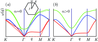
Figure 3: (a)Phonon spectrum for the undistorted kagome lattice. Dashed lines depict frequencies at $k^{\prime}=0$ and full lines at $k^{\prime}>0$. The inset shows the Brillouin zone with symmetry points $\Gamma$, $M$, and $K$. Note the line of zero modes along $\Gamma M$ when $k^{\prime}=0$, all of which develop nonzero frequencies for wavenumber $q>0$ when $k^{\prime}>0$ reaching $\omega^{*}\sim\sqrt{k^{\prime}}$ on a plateau beginning at $q\approx q^{*}\sim\sqrt{k^{\prime}}$ defining a length scale $l^{*}=1/q^{*}$. (b) Phonon spectrum for $\alpha>0$ and $k^{\prime}=0$. The plateau along $\Gamma M$ defines $\omega_{\alpha}\sim\sqrt{k}|\sin\alpha|$ and its onset at $q_{\alpha}\sim\omega_{\alpha}$ defines a length $l_{\alpha}\sim 1/|\sin\alpha|$.

IV Mode counting and states of self stress

To understand the origin of the differences in the zero-mode count for different boundary conditions, we turn to an elegant formulation Calladine1978 of the Maxwell rule that takes into account the existence of redundant bonds (i.e., bonds whose removal does not increase the number of floppy modes JacobsTho1995 ) and states in which springs can be under states of self-stress. Consider a ring network in two dimensions shown in Fig. 4 with $N=4$ nodes and $N_{b}=4$ springs with three springs of length $a$ and one spring of length $b$. The Maxwell count yields $N_{0}=4=3+1$ zero modes: two rigid translations, one rigid rotation, and one internal floppy mode – all of which are “finite-amplitude” modes with zero energy even for finite-amplitude displacements. When $b=3a$, the Maxwell rule breaks down. In the zero-energy configuration, the long spring and the three short ones are colinear, and a prestressed state in which the $b$-spring is under compression and the three $a$-springs are under tension (or vice versa) but the total force on each node remains zero becomes possible. This is called a state of self-stress. The system still has three finite amplitude zero modes corresponding to arbitrary rigid translations and rotations, but the finite-amplitude floppy mode has disappeared. In the absence of prestress, it is replaced by two “infinitesimal” floppy modes of displacements of the two internal nodes perpendicular of the now linear network. In the presence of prestress, these two modes have a frequency proportional to the square root of the tension in the springs. Thus, the system now has one state of self stress and one extra zero mode in the absence of prestress, implying $N_{0}=2N-N_{B}+S$, where $S$ is the number of states of self stress.

This simple count is more generally valid as can be shown with the aid of the equilibrium and compatibility matrices Calladine1978 , denoted, respectively, as $\mathbf{H}$ and $\mathbf{C}\equiv\mathbf{H}^{T}$. $\mathbf{H}$ relates the vector $\mathbf{t}$ of $N_{B}$ spring tensions to the vector $\mathbf{f}$ of $dN$ forces at nodes via $\mathbf{H}\cdot\mathbf{t}=\mathbf{f}$, and $\mathbf{C}$ relates the the vector $\mathbf{d}$ of $dN$ node displacements to the vector $\mathbf{e}$ of $N_{B}$ spring stretches via $\mathbf{C}\cdot\mathbf{d}=\mathbf{e}$. The dynamical matrix determining the phonon spectrum is $\mathbf{D}=k\mathbf{H}\cdot\mathbf{H}^{T}$. Vectors $\mathbf{t}_{0}$ in the null space of $\mathbf{H}$, ($\mathbf{H}\cdot\mathbf{t}_{0}=0$), describe states of self-stress whereas vectors $\mathbf{d}_{0}$ in the null space of $\mathbf{C}$ represent displacements with no stretch $\mathbf{e}$, i.e., modes of zero energy. Thus the nullspace dimensions of $\mathbf{H}$ and $\mathbf{C}$ are, respectively, $S$ and $N_{0}$. The rank-nullity theorem of linear algebra Birkhoff-Mac1998 states that the rank $r$ of a matrix plus the dimension of its null space equals its column number. Since the rank of a matrix and its transpose are equal, the $\mathbf{H}$ and $\mathbf{C}$ matrices, respectively, yield the relations $r+S=N_{B}$ and $r+N_{0}=dN$, implying $N_{0}=dN-N_{B}+S$. Under PBCs, locally isostatic lattices have $z=2d$ exactly, and the Maxwell rule yields $N_{0}=0$: there should be no zero modes at all. But we have just seen that both the square and undistorted kagome lattices under PBCs have of order $\sqrt{N}$ zero modes as calculated from the dynamical matrix, which, because it is derived from a harmonic theory, does not distinguish between infinitesimal and finite-amplitude zero modes. Thus, in order for there to be zero modes, there must be states of self-stress, in fact one state of self-stress for each zero mode.

In the square lattice under FBCs, $N=N_{x}N_{y}$ and $N_{B}=2N_{x}N_{y}-N_{x}-N_{y}$, there are no states of self stress, and $N_{0}=N_{x}+N_{y}$ zero modes depicted in Fig. 1(b). Under PBCs, the dimension of the nullspace of $\mathbf{H}$ is $S=N_{x}+N_{y}$, and there are also $N_{0}=S=N_{x}+N_{y}$ zero modes that are identical to those under FBCs. We have already seen that there are $N_{0}=2(N_{x}+N_{y})-1$ zero modes in the free undistorted kagome lattice. Direct evaluations HutchinsonFle2006 (See Text S1) of the dimension of the null spaces of $\mathbf{H}$ and $\mathbf{C}$ for the undistorted kagome lattice with PBCs yields $S=N_{0}=3N_{x}$ when $N_{x}=N_{y}$. The zero modes under PBCs are identical to those under FBCs except that the $2N_{x}-1$ modes associated with lines parallel to $\mathbf{e}_{2}$ under FBCs get reduced to $N_{x}$ modes because of the identification of apposite sides of the lattice required by the PBCs as shown in Fig. 1(a). Thus the modes of both the square and kagome lattices do not depend strongly on whether FCBs or PBCs are applied. Under RBC’s, however, the floppy modes of both disappear. The situation for the twisted kagome lattice is different. There are still $2(N_{x}+N_{y})-1$ zero modes under FBCs, but there are only two states of self stress under PBCs and thus only $N_{0}=S=2$ zero modes, as a direct evaluation of the null spaces of $\mathbf{H}$ and $\mathbf{C}$ verifies (See Appendix for details), in agreement with the results obtained via direct evaluation of the eigenvalues of the dynamical matrix SouslovLub2009 ; GuestHut2003 . All of the floppy modes under FBCs have disappeared.

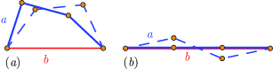
Figure 4: (a) Ring-network with $b>3a$ showing internal floppy mode. (b) Ring-network with $b=3a$ showing one of the two infinitesimal modes.

V Effective theory and edge modes

An effective long-wavelength energy $E_{\rm eff}$ for the low-energy acoustic phonons and nearly floppy distortions provides insight into the nature of the modes of the twisted kagome lattice. The variables in this theory are the vector displacement field $\mathbf{u}(\mathbf{x})$ of nodes at undistorted positions $\mathbf{x}$ and the scalar field $\phi(\mathbf{x})$ describing nearly floppy distortions within a unit cell. The detailed form of $E_{\rm eff}$ depends on which three lattice sites are assigned to a unit cell. Figure 1(c) depicts the lattice distortion $\phi$ for the nearly floppy mode at $\Gamma$ (with energy proportional to $|\sin\alpha|^{2}$) along with a particular representation of a unit cell, consisting of a central asymmetric hexagon and two equilateral triangles, with $8$ sites on its boundary. If sites $1$, $2$, and $3$ are assigned to the unit cell, then the distortion $\phi$ involves no rotations of these sites relative to their center of mass, and the harmonic limit of $E_{\rm eff}$ depends only on the symmetrized and linearized strain $u_{ij}=(\partial_{i}u_{j}+\partial_{j}u_{i})/2$ and on $\phi$:

$$E = \frac{1}{2}\int d^{2}x\Bigl{[}2\mu{\tilde{u}}_{ij}^{2}$$ (1)

$$+K(\phi+\xi u_{ii})^{2}+V(\partial_{i}\phi)^{2}-W\Gamma^{ijk}u_{ij}\partial_{k}\phi\Bigr{]},$$

where ${\tilde{u}}_{ij}=u_{ij}-\frac{1}{2}\delta_{ij}u_{kk}$ is the symmetric-traceless stain tensor, $\mu=\sqrt{3}k/8$, $K=3\sqrt{3}\tan^{2}\alpha/a^{2}$, $\xi=a\csc\alpha/(2\sqrt{3})$, $W=\sqrt{3}k/4+O(\alpha^{2})$, and $V=\sqrt{3}k/8+O(\alpha^{2})$. The last term in which $\Gamma^{ijk}$ is a third-rank tensor, whose only non-vanishing components are $\Gamma^{xxx}=-\Gamma^{xyy}=-\Gamma^{yyx}=-\Gamma^{xyx}=1$, is invariant under operations of the group $C_{6v}$ but not under arbitrary rotations. The $K\xi\phi u_{ii}$ term is the only one that reflects the $C_{3v}$ (rather than $C_{6v}$) symmetry of the lattice. There are several comments to make about this energy. The gauge-like coupling in which the isotropic strain $u_{ii}$ appears only in the combination $(\phi+\xi u_{ii})^{2}$ guarantees that the bulk modulus vanishes: $\phi$ will simply relax to $-\xi u_{ii}$ to reduce to zero the energy of any state with nonvanishing $u_{ii}$. The coefficient $K$ can be calculated directly from the observation that under $\phi$ alone, the length of every spring changes by $\delta a=-\sqrt{3}\phi\sin\alpha$, and this length change is reversed by a homogenous volume change $u_{ii}=\delta A_{\alpha}/A_{\alpha}=-2\delta a/a$. In the $\alpha\to 0$ limit, $K\to 0$, and the energy reduces to that of an isotropic solid with bulk modulus $B_{0}=\lim_{\alpha\to 0}K\xi^{2}=\sqrt{3}k/4$ if the $V$ and $W$ terms, which are higher order in gradients, are ignored. The $W$ term gives rise to a term, singular in gradients of $\mathbf{u}$, when $\phi$ is integrated out that is responsible for the deviations of the finite-wavenumber elastic energy from isotropy. At small $\alpha$, the length scale $l_{\alpha}$ appears in several places in this energy: in the length $\xi$ and in the ratios $\sqrt{\mu/K}$, $\sqrt{V/K}$, and $\sqrt{W/K}$. At length scales much larger than $l_{\alpha}$, the $V$ and $W$ terms can be ignored, and $\phi$ relaxes to $-\xi u_{ii}$ leaving only the shear elastic energy of an elastic solid proportional $\mu\tilde{u}_{ij}^{2}$. At length scales shorter than $l_{\alpha}$, $\phi$ deviates from $-\xi u_{ii}$ and contributes significantly to the form of the energy spectrum. If $1$, $2^{*}$ and $3^{*}$ in Fig. 1(d) are assigned to the unit cell, then $\phi$ involves rotations relative to the lattice axes, and the energy develops a Cosserat-like form Cosserat1909 ; Kunin1983 that is a function of $\phi-a({\boldsymbol{\nabla}}\times\mathbf{u})_{z}/2$ rather than $\phi$.

The modes of our elastic energy in the long-wavelength limit ($ql_{\alpha}\ll 1$) are simply those of an elastic medium with $B=0$. In this limit, there are transverse and longitudinal bulk sound modes with equal sound velocities $c_{T}=\sqrt{\mu/\rho}=(a/2)\sqrt{k/m}$ and $c_{L}=\sqrt{(B+\mu)/\rho}\to c_{T}$, where $m$ is the particle mass at each node and $\rho$ is the mass density. In addition there are Rayleigh surface waves Landau-elasticity in which there is a single decay length (rather than the two at $B>0$), and displacements are proportional to $e^{-q_{y}y}\cos[q_{x}x]$ with $q_{y}=q_{x}$ for a semi-infinite sample in the right half plane so that the penetration depth into the interior is $1/q_{x}$. These waves have zero frequency in two dimensions when $B=0$, and they do not appear in the spectrum with PBCs. Thus this simple continuum limit provides us with an explanation for the difference between the spectrum of the free and periodic twisted kagome lattices. Under FBCs, there are zero-frequency surface modes not present under PBCs.

Further insight into how boundary conditions affect spectrum follows from the observation that the continuum elastic theory with $B=0$ depends only on $\tilde{u}_{ij}$. The metric tensor $g_{ij}(\mathbf{x})$ of the distorted lattice is related to the strain $u_{ij}(\mathbf{x})$ via the simple relation $g_{ij}(\mathbf{x})=\delta_{ij}+2u_{ij}(\mathbf{x})$; and $\tilde{u}_{ij}=[g_{ij}(\mathbf{x})-\frac{1}{2}\delta_{ij}g_{kk}(\mathbf{x})]/2$, which is zero for $g_{ij}=\delta_{ij}$, is invariant, and thus remains equal to zero, under conformal transformations that take the metric tensor from its reference form $\delta_{ij}$ to $h(\mathbf{x})\delta_{ij}$ for any continuous function $h(\mathbf{x})$. The zero modes of the theory thus correspond simply to conformal transformations, which in two dimensions are best represented by the complex position and displacement variables $z=x+iy$ and $w(z)=u_{x}(z)+iu_{y}(z)$. All conformal transformations are described by an analytic displacement field $w(z)$. Since by Cauchy’s theorem, analytic functions in the interior of a domain are determined entirely by their values on the domain’s boundary (the “holographic” property Susskind1995 ), the zero modes of a given sample are simply those analytic functions that satisfy its boundary conditions. For example, a disc with fixed edges ($\mathbf{u}=0$) has no zero modes because the only analytic function satisfying this FBC is the trivial one $w(z)=0$; but a disc with free edges (stress and thus strain equal to zero) has one zero mode for each of the analytic functions $w(z)=a_{n}z^{n}$ for integer $n\geq 0$. The boundary conditions $\lim_{x\to\infty}\mathbf{u}(x,y)=0$ and $\mathbf{u}(x,y)=\mathbf{u}(x+L,y)$ on a semi-infinite cylinder with axis along $x$ are satisfied by the function $w(z)=e^{iq_{x}z}=e^{iq_{x}x}e^{-q_{x}y}$ when $q_{x}=2n\pi/L$, where $n$ is an integer. This solution is identical to that for classical Rayleigh waves on the same cylinder. Like the Rayleigh theory, the conformal theory puts no restriction on the value of $n$ (or equivalently $q_{x}$). Both theories break down, however, at $q_{x}=q_{c}\approx\min(l_{\alpha}^{-1},a^{-1})$ beyond which the full lattice theory, which yields a complex value of $q_{y}=q_{y}^{\prime}+iq_{y}^{\prime\prime}$, is needed.

Figure 5(a) shows an example of a surface wave. At the bottom of this figure, $u_{y}(x)$ is an almost perfect sinusoid. As $y$ decreases toward the surface, the amplitude grows, and in this picture reaches the nonlinear regime by the time the surface at $y=0$ is reached. Figure 5(b) plots $q_{y}^{\prime}$ as a function of $q_{x}$ obtained both by direct numerical evaluation and by an analytic transfer matrix procedure LeeJoa1981-2 for different values of $\alpha$ (Text S1). The Rayleigh limit $q_{y}^{\prime}=q_{x}$ is reached for all $\alpha$ as $q_{x}\to 0$. Interestingly the Rayleigh limit remains a good approximation up to values of $q_{x}$ that increase with increasing $\alpha$. The inset to Fig. 5, plots $q_{y}^{\prime}l_{\alpha}$ as a function of $\eta=q_{x}l_{\alpha}$ and shows that in the limit $\alpha\to 0$ ($l_{\alpha}/a\to\infty$), $q_{y}^{\prime}$ obeys an $\alpha$-independent scaling law of the form $q_{y}^{\prime}=l_{\alpha}^{-1}f(q_{x}l_{\alpha})$. The full complex $q_{y}$ obeys a similar equation. This type of behavior is familiar in critical phenomena where scaling occurs when correlation lengths become much larger than microscopic lengths. The function $f(\eta)$ approaches $\eta$ as $\eta\to 0$ and asymptotes to $4/3$ for $\eta\to\infty$. Thus for $q_{x}l_{\alpha}\ll 1$, $q_{y}^{\prime}=q_{x}$ and for $q_{x}l_{\alpha}\gg 1$, $q_{y}^{\prime}=(4/3)l_{\alpha}^{-1}$. As $\alpha$ increases, $l_{\alpha}/a$ is no longer much larger than one, and deviations from the scaling law result. The situation for surfaces along different directions (e.g., along $x=0$ rather than $y=0$) is more complicated and will be treated in a future publication SunLub2011 .

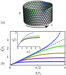
Figure 5: (a)Lattice distortions for a surface wave on a cylinder, showing exponential decay of the surface displacements into the bulk. This figure was constructed by specifying a small sinusoidal modulation on the bottom boundary and propagating lattice-site positions upward to the free boundary at the top under the constraint of of constant lengths and periodic boundary conditions around the cylinder. Distortions near and at the top boundary, which have become nonlinear, are not described by our linearized treatment. (b) $q_{y}^{\prime}a_{L}$ as a function of $q_{x}a_{L}$ for lattice Rayleigh surface waves for $\alpha=\pi/20,\pi/10,3\pi/20,\pi/5,\pi/4$, in order from bottom to top. Smooth curves are the analytic results from a transfer matrix calculation, and dots are from direct numerical calculations. The dashed line is the continuum Rayleigh limit $q_{y}^{\prime}=q_{x}$. Curves at smaller $\alpha$ break away from this curve at smaller values of $q_{y}$ than do those at large $\alpha$. At $\alpha=\pi/4$, $q_{x}^{\prime}$ diverges at $q_{y}a_{L}=\pi$. The inset plots $q_{y}^{\prime}l_{\alpha}$ as a function of $q_{x}l_{\alpha}$ for different $\alpha$. The lower curve in the inset(black) is the $\alpha$-independent scaling function of $q_{y}l_{\alpha}$ reached in the $\alpha\to 0$ limit. The other curves from top to bottom are for $\alpha=\pi/25$, $\pi/12$, $\pi/9$, and $\pi/6$ (chosen to best present results rather than to match the curves in the main figure). Curves for $\alpha<\pi/15$ are essentially indistinguishable from the scaling limit. The curve at $\alpha=\pi/6$ stops because $q_{y}<\pi/a_{L}$.

VI Other lattices and relation to jamming

The $C_{3v}$ twisted kagome lattice is the simplest of many lattices that can be formed from the kagome and other periodic isostatic lattices. Figures 6 (a) and (b) show two other examples of isostatic lattices constructed from the kagome lattice. Most intriguing is the lattice with pgg symmetry. Its geometry has uniaxial symmetry, yet its long-wavelength elastic energy is identical to that of the $C_{3v}$ twisted kagome lattice, i.e, it is isotropic with a vanishing bulk modulus, and its mode structure near $\mathbf{q}=0$ is isotropic as shown in Fig. 6 (c). Thus, this system loses long-wavelength zero-frequency bulk modes of the undistorted kagome lattice to surface modes. However, at large wavenumber, lattice anisotropy becomes apparent, and (infinitesimal) floppy bulk modes appear. Thus in this and related systems, a fraction of the zero modes of the under FBCs are bulk modes that are visible under PBCs, and a fraction are surface modes that are not.

Randomly packed spheres above the jamming transition with average coordination number $z=2d+\Delta z$ exhibit a characteristic frequency $\omega^{*}\sim\Delta z$ and length $l^{*}\sim(\Delta z)^{-1}$ and a transition from a Debye-like ($\sim\omega^{d-1}$) to a flat density of states at $\omega\approx\omega^{*}$ OhernNag2003 ; SilbertNag2005 . The square and kagome lattices with randomly added $NNN$ springs have the same properties MaoLub2010 ; MaoLub2011a . A general “cutting” argument Wyartwit2005b ; Wyart2005 provides a procedure for perturbing away from the isostatic limit and an explanation for these properties. However, it only applies provided a finite fraction of the of order $L^{d-1}$ floppy modes of a sample with sides of length $L$ cut from an isostatic lattice with PBCs are extended, i.e., have wave functions that extend across the sample rather than remaining localized either in the interior or at the surface the sample. Clearly the twisted kagome lattice, whose floppy modes are all surface modes, violates this criterion; and indeed, the density of states of the lattice with $\Delta z=0$ shows Debye-behavior crossing over to a flat plateau at $\omega\approx\omega_{\alpha}$. Adding next nearest neighbor bonds gives rise to a length $l_{c}\approx(l_{\alpha}^{-1}+l^{*-1})^{-1}$ and crossover to the plateau at $\omega_{c}\sim l_{c}^{-1}$. The pgg lattice in Fig. 6(a), however, has both extended and surface floppy modes, so its crossover to the a flat plateau occurs at $\omega\approx\omega^{*}$ rather than at $\omega_{\alpha}$ or $\omega_{c}$.

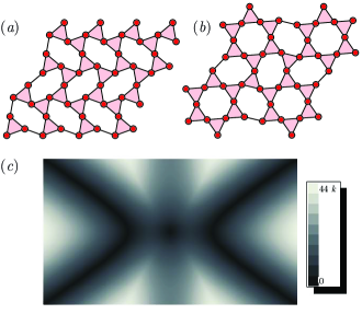
Figure 6: (a) Kagome-based lattice with pgg space group symmetry and uniaxial $c_{2v}$ point group symmetry. (b) Lattice with p6 space symmetry but global $C_{6}$ point-group symmetry. (c) Density plot of the spectrum of the lowest frequency branch of the pgg uniaxial kagome lattice. The spectrum is absolutely isotropic near the origin point $\Gamma$, but it has a zero modes on two symmetry related continuous curves at large values of wave-number.

VII Connections to other systems

Our study highlights the rich and remarkable variety of physical properties that isostatic systems can exhibit. Under FBCs, floppy modes can adopt a variety of forms, from all being extended to all being localized near surfaces to a mixture of the two. Under PBC’s, the presence of floppy modes depends on whether the lattice can or cannot support states of self stress. When a lattice exhibits a large number of zero-energy edge modes, its mechanical/dynamical properties become extremely sensitive to boundary conditions, much as do the electronic properties of the topological states of matter studied in

quantum systems KaneFisher1997 ; Jain2007 ; HasanKane2010 ; QiZhang2011 . The zero-energy edge modes observed in our isostatic lattices are collective modes whose amplitudes decay exponentially from the edge with a finite decay length, in direct contrast to the very localized and trivial floppy modes arising from dangling bonds. We focussed primarily on high-symmetry lattices derived from the kagome lattice, but the properties they exhibit, namely a deficit of floppy modes in the bulk and the existence of floppy surface modes, are shared by any two-dimensional system with a vanishing bulk modulus (or the equivalent in anisotropic systems). Three-dimensional analogs of the twisted kagome lattice SouslovLub2011 can be constructed by rotating tetrahedra in pyrochlore and zeolite lattices Zeolitereview ; SartbaevaTho2006 and in cristobalites HammondsWin1996 . These lattices are anisotropic. With $NN$ forces only, they exhibit a vanishing modulus for compression applied in particular planes rather than isotropically, but we expect them to exhibit many of the properties the two-dimensional lattices exhibit. Finally, we note that Maxwell’s ideas can be applied to spin systems such as the Heisenberg anti-ferromagnet on the kagome lattice MoessnerCha1998 ; Lawler2011 , and the possibility of unusual edge states in them is intriguing.

Appendix A Derivation of equilibrium, compatibility, and dynamical matrices.

In this section, we will provide some of the details for calculating the equilibrium and compatibility matrices $\mathbf{H}$ and $\mathbf{C}$ and the Dynamical matrix $\mathbf{D}$ under periodic boundary conditions. The equilibrium matrix $\mathbf{H}$ relates the $N_{B}=dN$ dimensional vector of bond tensions $\mathbf{t}$ to the $dN$ dimensional vector $\mathbf{f}$ of forces at the nodes via $\mathbf{H}\cdot\mathbf{t}=\mathbf{f}$. We label unit cells by the their position vectors $\mathbf{l}=l_{1}\mathbf{e}_{1}+l_{2}\mathbf{e}_{2}$, where $l_{1}$ and $l_{2}$ are integers and

$$\mathbf{e}_{n}=(\cos\phi_{n},\sin\phi_{n});\qquad\phi_{n}=\frac{2\pi(n-1)}{3}$$ (2)

are the primitive lattice vectors. (Here we take the lattice spacing to be one, i.e., $2a\cos\alpha\to 1$.) Each unit cell has three sites, labeled $1$, $2$, and $3$ as shown in Fig. 7, so we label the $3N_{c}$ sites by $(\mathbf{l},a)$, where $a=1,2,3$ and $N_{c}=N/3$ is the number of unit cells. Forces at the nodes are denoted by $\mathbf{f}_{\mathbf{l},a}$ and their $6N_{c}=2N$ components as $\mathbf{f}_{\mathbf{l},a,i}$, where $i=x,y$. They have to be balanced by stretching forces in the springs located on the bonds. There are six bonds per cell, which we can take to be the six bonds in the distorted hexagon shown in Fig. 7, oriented parallel to the unit vectors

$$\mathbf{b}_{n}(\alpha)=(\cos\psi_{n},\sin\psi_{n});\qquad\psi_{n}=\frac{(n-1)\pi}{3}+(-1)^{n}\alpha$$ (3)

for $n=1,...,6$, where $\alpha$ is the twist angle of the twisted kagome lattice. When $\alpha=0$, these vector reduce to the edge vectors of a symmetric hexagon with $\mathbf{b}_{p}(0)=-\mathbf{b}_{p+3}(0)$.

The $6N_{c}=2N$ bonds, labeled with $\mathbf{l},n$, are occupied by springs under tension $t_{\mathbf{l},n}$ that exert pulling (for $t_{\mathbf{l},n}>0$) forces, direct along the bond vectors $\pm\mathbf{b}_{n}(\alpha)$, on nodes. We define vectors $\mathbf{t}_{\mathbf{l},n}=t_{\mathbf{l},n}\mathbf{b}_{n}(\alpha)$. Because we have periodic boundary conditions, we can express both $\mathbf{f}_{\mathbf{l},a}$ and $\mathbf{t}_{\mathbf{l},n}$ in terms of their Fourier components,

$$\mathbf{f}_{\mathbf{l},a} = \frac{1}{\sqrt{N_{c}}}\sum_{\mathbf{q}}e^{i\mathbf{q}_{\cdot}\mathbf{l}}\mathbf{f}_{\mathbf{q},n}$$ (4)

$$\mathbf{t}_{\mathbf{l},n} = \frac{1}{\sqrt{N_{c}}}\sum_{\mathbf{q}}e^{i\mathbf{q}_{\cdot}\mathbf{l}}\mathbf{t}_{\mathbf{q},n}.$$ (5)

The equilibrium matrix is diagonal in $\mathbf{q}$, so it breaks up into independent $6\times 6$ blocks for each of the $N_{c}=N_{x}N_{y}$ independent vectors $\mathbf{q}$. For simplicity, we consider only the case $N_{x}=N_{y}$ for which $N_{c}=N_{x}^{2}$ and for which the number of sites is $N=3N_{x}^{2}$.

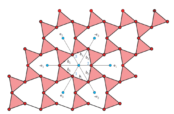
Figure 7: Watch this space

A.1 The Equilibrium Matrix

There are four bonds incident on each site. The equations relating $\mathbf{f}_{\mathbf{l},a}$ to $\mathbf{t}_{\mathbf{l},n}$ follow from Fig. 7:

$$\mathbf{f}_{\mathbf{l},1} = \mathbf{t}_{\mathbf{l},1}-\mathbf{t}_{\mathbf{l},6}+\mathbf{t}_{\mathbf{l}+\mathbf{e}_{3},4}-\mathbf{t}_{\mathbf{l}+\mathbf{e}_{3},3}$$ (6)

$$\mathbf{f}_{\mathbf{l},2} = \mathbf{t}_{\mathbf{l},3}-\mathbf{t}_{\mathbf{l},2}+\mathbf{t}_{\mathbf{l}+\mathbf{e}_{1},6}-\mathbf{t}_{\mathbf{l}+\mathbf{e}_{1},5}$$ (7)

$$\mathbf{f}_{\mathbf{l},3} = \mathbf{t}_{\mathbf{l},5}-\mathbf{t}_{\mathbf{l},4}+\mathbf{t}_{\mathbf{l}+\mathbf{e}_{2},2}-\mathbf{t}_{\mathbf{l}+\mathbf{e}_{2},1}.$$ (8)

We map $(a,i)$ to a single index $m$ with $(a,x)\to 2a-1$ and $(a,y)\to 2a$ and then Fourier transform. The result is that $\mathbf{H}$ breaks up into independent $6\times 6$ blocks $\mathbf{H}_{nm}(\mathbf{q})$ for each $\mathbf{q}$. This leads to

$$f_{n}(\mathbf{q})=H_{n,m}(\mathbf{q})t_{m}(\mathbf{q}),$$ (9)

where

$$\mathbf{H}(\mathbf{q})=\begin{pmatrix}b_{1,x}(\alpha)&0&-e^{i\mathbf{q}\cdot\mathbf{e}_{3}}b_{3,x}(\alpha)&e^{i\mathbf{q}\cdot\mathbf{e}_{3}}b_{4,x}(\alpha)&0&-b_{6,x}(\alpha)\\ b_{1,y}(\alpha)&0&-e^{i\mathbf{q}\cdot\mathbf{e}_{3}}b_{3,y}(\alpha)&e^{i\mathbf{q}\cdot\mathbf{e}_{3}}b_{4,y}(\alpha)&0&-b_{6,y}(\alpha)\\ 0&-b_{2,x}(\alpha)&b_{3,x}(\alpha)&0&-e^{i\mathbf{q}\cdot\mathbf{e}_{1}}b_{5,x}(\alpha)&e^{i\mathbf{q}\cdot\mathbf{e}_{1}}b_{6,x}(\alpha)\\ 0&-b_{2,y}(\alpha)&b_{3,y}(\alpha)&0&-e^{i\mathbf{q}\cdot\mathbf{e}_{1}}b_{5,y}(\alpha)&e^{i\mathbf{q}\cdot\mathbf{e}_{1}}b_{6,y}(\alpha)\\ -e^{i\mathbf{q}\cdot\mathbf{e}_{2}}b_{2,x}(\alpha)&e^{i\mathbf{q}\cdot\mathbf{e}_{2}}b_{1,x}(\alpha)&0&b_{5,x}(\alpha)&-b_{4,x}(\alpha)&0\\ -e^{i\mathbf{q}\cdot\mathbf{e}_{2}}b_{2,y}(\alpha)&e^{i\mathbf{q}\cdot\mathbf{e}_{2}}b_{1,y}(\alpha)&0&b_{5,y}(\alpha)&-b_{4,y}(\alpha)&0\end{pmatrix}.$$ (10)

The null space of this matrix is easily calculated with the aid of Mathematica.

Case 1, $\alpha=0$: This is the untwisted kagome lattice. When $\mathbf{q}\neq 0$, the null space of $\mathbf{H}(\mathbf{q})$ is empty unless $\mathbf{q}$ is perpendicular to one of the primitive lattice vectors:

$$\mathbf{q}=q_{\perp,n}\mathbf{e}_{\perp,n}=q(-\sin\phi_{n},\cos\phi_{n}),\qquad n=1,2,3,$$ (11)

and $\mathbf{q}\cdot\mathbf{e}_{n}=q_{||,n}=0$, in which case there is a single vector,

$$t_{1}(\mathbf{q}) = \sqrt{N_{c}}\delta_{q_{||,1},0}(1,0,0,e^{-iq_{\perp,1}\,\mathbf{e}_{3}\cdot\mathbf{e}_{\perp,1}},0,0)$$ (12)

$$t_{2}(\mathbf{q}) = \sqrt{N_{c}}\delta_{q_{||,2},0}(0,1,0,0,e^{-iq_{\perp,2}\,\mathbf{e}_{1}\cdot\mathbf{e}_{\perp,2}},0)$$ (13)

$$t_{3}(\mathbf{q}) = \sqrt{N_{c}}\delta_{q_{||,3},0}(0,0,1,0,0,e^{-iq_{\perp,3}\,\mathbf{e}_{2}\cdot\mathbf{e}_{\perp,3}}),$$ (14)

where $N_{c}$ is the number of cells, for each $n$ and $q_{\perp,n}$ in the null space. When $\mathbf{q}=0$, there are three vectors, $(1,0,0,1,0,0)$, $(0,1,0,0,1,0)$, and $(0,0,1,0,0,1)$ in the null space. These are the $q=0$ limits of $t_{1}(\mathbf{q})$, $t_{2}(\mathbf{q})$, and $t_{3}(\mathbf{q})$, respectively. We can, therefore, take the set of null-space vectors of $\mathbf{H}$ to be $t_{1}(\mathbf{q})$, $t_{2}(\mathbf{q})$, and $t_{2}(\mathbf{q})$ for the $N_{x}$ values of $q$, which include $q=0$. Linear combinations of these vectors are also null-space vectors, and we can use them to construct vectors confined to a single line of bonds. For example the vector

$$t_{1}(\mathbf{l})=\frac{1}{N_{c}}\sum_{q}e^{i\mathbf{q}\cdot\mathbf{l}}t_{1}(\mathbf{q})=(\delta_{l_{y},0},0,0,\delta_{l_{y},-\sqrt{3}/2},0,0)$$ (15)

corresponds to a state in which springs on all $1$-bond in cells with centers at $\mathbf{l}=l_{1}\mathbf{e}_{1}$ for any $l_{1}$ and on all $4$-bonds in cells with centers at $\mathbf{l}=l_{1}\mathbf{e}_{1}+\mathbf{e}_{3}=(l_{1}-(1/2),-\sqrt{3}/2)$ are all under the same tension. This is a state of self-stress in which all bonds along a particular straight line parallel to the $\mathbf{e}_{1}$-axis are under tension. Similar states of self-stress for any of the $3N_{x}$ lines of bonds can be constructed.

Case 2, $\alpha>0$: This is the twisted lattice. The null space of $\mathbf{H}(\mathbf{q})$ is empty for all $\mathbf{q}>0$, and it contains only two vectors when $\mathbf{q}=0$. These correspond to two states of self-stress in which the stress the stress on the six bonds take on both positive and negative values that are identical in all unit cells.

A.2 The Compatibility Matrix

The compatibility matrix $\mathbf{C}$ relates the $dN$ displacements $\mathbf{d}$ to the $N_{b}$ stretches $\mathbf{s}_{\mathbf{l},a}$. The displacements are labeled the same way as the forces, i.e. as $\mathbf{d}_{\mathbf{l},a}$ and the stretches in the same way as the bond tensions, i.e. as $s_{\mathbf{l},n}$. The equations relating $\mathbf{d}_{\mathbf{l},a}$ and $\mathbf{s}_{\mathbf{l},n}\equiv-s_{\mathbf{l},n}\mathbf{b}_{n}(\alpha)$ are

$$\mathbf{d}_{\mathbf{l}-\mathbf{e}_{2},3}-\mathbf{d}_{\mathbf{l},1} = \mathbf{s}_{\mathbf{l},1}=-s_{\mathbf{l},1}\mathbf{b}_{1}(\alpha)$$

$$\mathbf{d}_{\mathbf{l},2}-\mathbf{d}_{\mathbf{l}-\mathbf{e}_{2},3} = \mathbf{s}_{\mathbf{l},2}=-s_{\mathbf{l},2}\mathbf{b}_{2}(\alpha)$$

$$\mathbf{d}_{\mathbf{l}-\mathbf{e}_{3},1}-\mathbf{d}_{\mathbf{l},2} = \mathbf{s}_{\mathbf{l},3}=-s_{\mathbf{l},3}\mathbf{b}_{3}(\alpha)$$

$$\mathbf{d}_{\mathbf{l},3}-\mathbf{d}_{\mathbf{l}-\mathbf{e}_{3},1} = \mathbf{s}_{\mathbf{l},4}=-s_{\mathbf{l},4}\mathbf{b}_{4}(\alpha)$$

$$\mathbf{d}_{\mathbf{l}-\mathbf{e}_{1},2}-\mathbf{d}_{\mathbf{l},3} = \mathbf{s}_{\mathbf{l},5}=-s_{\mathbf{l},5}\mathbf{b}_{5}(\alpha)$$

$$\mathbf{d}_{\mathbf{l},1}-\mathbf{d}_{\mathbf{l}-\mathbf{e}_{1},2} = \mathbf{s}_{\mathbf{l},6}=-s_{\mathbf{l},6}\mathbf{b}_{6}(\alpha).$$ (16)

Fourier transforming and using the same $(n,m)$ notation as for the equilibrium matrix, we obtain

$$\mathbf{C}_{mn}(\mathbf{q})d_{n}(\mathbf{q})=s_{m}(\mathbf{q}),$$ (17)

where $\mathbf{C}_{mn}(\mathbf{q})=\mathbf{H}_{nm}(-\mathbf{q})=\mathbf{H}_{mn}^{\dagger}(\mathbf{q})$ as required by the constraint $\mathbf{C}=\mathbf{H}^{T}$.

A.3 The Dynamical Matrix

Finally, the dynamical matrix is $\mathbf{D}(\mathbf{q})=k\mathbf{H}(\mathbf{q})\cdot\mathbf{C}(\mathbf{q})$, whose components are

$$D_{11}(\mathbf{q}) = \frac{1}{2}[\cos(2\alpha)+4]$$

$$D_{12}(\mathbf{q}) = =-\frac{1}{2}\sqrt{3}\cos(2\alpha)$$

$$D_{13}(\mathbf{q}) = =D_{31}^{*}(\mathbf{q})=-e^{-i\left(\frac{q_{x}}{2}+\frac{\sqrt{3}q_{y}}{2}\right)}\sin^{2}\left(\frac{\pi}{6}-\alpha\right)-e^{-iq_{x}}\sin^{2}\left(\alpha+\frac{\pi}{6}\right)$$

$$D_{14}(\mathbf{q}) = D_{41}^{*}(\mathbf{q})=\frac{1}{2}e^{-iq_{x}}\cos\left(\frac{\pi}{6}-2\alpha\right)+\frac{1}{2}e^{-i\left(\frac{q_{x}}{2}+\frac{\sqrt{3}q_{y}}{2}\right)}\cos\left(2\alpha+\frac{\pi}{6}\right)$$

$$D_{15}(\mathbf{q}) = D_{51}^{*}(\mathbf{q})=-2e^{-\frac{1}{2}i\sqrt{3}q_{y}}\cos^{2}(\alpha)\cos\left(\frac{q_{x}}{2}\right)$$

$$D_{16}(\mathbf{q}) = D_{61}^{*}(\mathbf{q})=ie^{-\frac{1}{2}i\sqrt{3}q_{y}}\sin(2\alpha)\sin\left(\frac{q_{x}}{2}\right)$$

$$D_{22}(\mathbf{q}) = 2\sin^{2}(\alpha)+\cos^{2}\left(\frac{\pi}{6}-\alpha\right)+\cos^{2}\left(\alpha+\frac{\pi}{6}\right)$$

$$D_{23}(\mathbf{q}) = D_{32}^{*}(\mathbf{q})=\frac{1}{2}e^{-iq_{x}}\cos\left(\frac{\pi}{6}-2\alpha\right)+\frac{1}{2}e^{-i\left(\frac{q_{x}}{2}+\frac{\sqrt{3}q_{y}}{2}\right)}\cos\left(2\alpha+\frac{\pi}{6}\right)$$

$$D_{24}(\mathbf{q}) = D_{42}^{*}(\mathbf{q})=-e^{-i\left(\frac{q_{x}}{2}+\frac{\sqrt{3}q_{y}}{2}\right)}\cos^{2}\left(\frac{\pi}{6}-\alpha\right)-e^{-iq_{x}}\cos^{2}\left(\alpha+\frac{\pi}{6}\right)$$

$$D_{2,5}(\mathbf{q}) = D_{5,2}^{*}(\mathbf{q})=ie^{-\frac{1}{2}i\sqrt{3}q_{y}}\sin(2\alpha)\sin\left(\frac{q_{x}}{2}\right)$$

$$D_{2,6}(\mathbf{q}) = D_{6,2}^{*}(\mathbf{q})=-2e^{-\frac{1}{2}i\sqrt{3}q_{y}}\sin^{2}(\alpha)\cos\left(\frac{q_{x}}{2}\right)$$

$$D_{33}(\mathbf{q}) = 2\sin^{2}\left(\frac{\pi}{6}-\alpha\right)+2\sin^{2}\left(\alpha+\frac{\pi}{6}\right)$$

$$D_{34}(\mathbf{q}) = D_{43}^{*}(\mathbf{q})=0$$

$$D_{3,5}(\mathbf{q}) = D_{5,3}(\mathbf{q})=-e^{-i\left(\frac{\sqrt{3}q_{y}}{2}-\frac{q_{x}}{2}\right)}\sin^{2}\left(\frac{\pi}{6}-\alpha\right)-e^{iq_{x}}\sin^{2}\left(\alpha+\frac{\pi}{6}\right)$$

$$D_{3,6}(\mathbf{q}) = D_{6,3}^{*}(\mathbf{q})=-\frac{1}{2}e^{iq_{x}}\cos\left(\frac{\pi}{6}-2\alpha\right)-\frac{1}{2}e^{i\left(\frac{q_{x}}{2}-\frac{\sqrt{3}q_{y}}{2}\right)}\cos\left(2\alpha+\frac{\pi}{6}\right)$$

$$D_{4,4}(\mathbf{q}) = 2\cos^{2}\left(\frac{\pi}{6}-\alpha\right)+2\cos^{2}\left(\alpha+\frac{\pi}{6}\right)$$

$$D_{4,5}(\mathbf{q}) = D_{5,4}^{*}(\mathbf{q})=-\frac{1}{2}e^{iq_{x}}\cos\left(\frac{\pi}{6}-2\alpha\right)-\frac{1}{2}e^{i\left(\frac{q_{x}}{2}-\frac{\sqrt{3}q_{y}}{2}\right)}\cos\left(2\alpha+\frac{\pi}{6}\right)$$

$$D_{4,6}(\mathbf{q}) = D_{6,4}^{*}(\mathbf{q})=-e^{i\left(\frac{q_{x}}{2}-\frac{\sqrt{3}q_{y}}{2}\right)}\cos^{2}\left(\frac{\pi}{6}-\alpha\right)-e^{iq_{x}}\cos^{2}\left(\alpha+\frac{\pi}{6}\right)$$

$$D_{5,5}(\mathbf{q}) = \sin^{2}\left(\frac{\pi}{6}-\alpha\right)+\sin^{2}\left(\alpha+\frac{\pi}{6}\right)+2\cos^{2}(\alpha)$$

$$D_{5,6}(\mathbf{q}) = D_{6,5}^{*}(\mathbf{q})=\frac{1}{2}\cos\left(\frac{\pi}{6}-2\alpha\right)+\frac{1}{2}\cos\left(2\alpha+\frac{\pi}{6}\right)$$

$$D_{6,6}(\mathbf{q}) = 2\sin^{2}(\alpha)+\cos^{2}\left(\frac{\pi}{6}-\alpha\right)+\cos^{2}\left(\alpha+\frac{\pi}{6}\right)$$ (18)

Its eigenvalue spectrum can easily be calculated with the aid of Mathematica. The results are shown in Fig. 3 of the main text.

Appendix B Surface Modes

Surface modes decay exponentially into the bulk. They are characterized by a wavevector $\mathbf{q}_{||}$ parallel to the plane of the surface, their frequency $\omega_{s}(\mathbf{q}_{||})$, their decay length $l(\mathbf{q}_{||})$ perpendicular to the surface. In lattices with nearest-neighbor forces only, $\omega_{s}(\mathbf{q}_{||})$ and $l(\mathbf{q}_{||})$ can be determined by setting $\mathbf{q}=\mathbf{q}_{||}+\mathbf{q}_{\perp}$, where $\mathbf{q}$ is the wavevector that appears in the dynamical matrix and $\mathbf{q}_{\perp}\equiv q_{\perp}\mathbf{e}_{\perp}$ is the component of $\mathbf{q}$ perpendicular to the surface ($\mathbf{e}_{\perp}$ is the unit vector perpendicular to the surface), setting $q_{\perp}=il^{-1}$, requiring

$$\det[\omega^{2}I-D(\mathbf{q}_{||},il^{-1})]=0,$$ (19)

where $I$ is the unit matrix, and that the equation of motion of the surface layer be satisfied. In the case of surface modes of with zero frequency, the relation $\det[D(\mathbf{q}_{||},il^{-1})]=0$ determines $l$ as a function of $\mathbf{q}_{||}$. The surface modes of the twisted kagome lattice have zero frequency, so we need only solve this equation. We consider only the case in which the surface is perpendicular to the $y$-direction and set $q_{x}=q$ and $r=e^{i\sqrt{3}q_{y}/2}\equiv e^{-\sqrt{3}/(2l)}$. We find

$$\det[D(q,r)]=\frac{9}{64}a(q)\left[r+r^{-1}-2g(q)\right]\left[r+r^{-1}-2g^{*}(q)\right],$$ (20)

where

$$a(q) = 2[2-\cos q+(1-2\cos q)\cos(4\alpha)]$$ (21)

$$g(q) = \frac{\cos(q/2)[3-2\cos p+\cos p\cos(4\alpha)]+2i\sqrt{3}\sin^{3}(3q/2)\sin(4\alpha)}{2-\cos q+(1-2\cos q)\cos(4\alpha)}$$ (22)

Solving for $r$ in Eq. (20) and to a lattice spacing of $2a\cos\alpha$, we obtain

$$k_{y}\equiv l^{-1}=\frac{1}{a\sqrt{3}\cos\alpha}\log[-g(2aq\cos\alpha)+\sqrt{g(2aq\cos\alpha)^{2}-1}].$$ (23)

This is the function that is plotted in Fig. 5(b) in the text. Note that $k_{y}$ has both a real and an imaginary part, but that in the limit $q\to 0$, $k_{y}=q$.

References

- (1) M. F. Thorpe, J. Non-Cryst. Solids 57, 355 (1983).
- (2) C. R. Calladine, Int. J. Solids and Structures 14,161 (1978).
- (3) S. Feng and P. N. Sen Phys. Rev. Lett. 52, 216 (1984).
- (4) D. J. Jacobs and M. F. Thorpe, Phys. Rev. Lett. 75, 4051 (1995).
- (5) J. Heyman, The Science of Structural Engineering (Cengage Learning, Stamford CT,2005).
- (6) A. Kassimali, Structural Analysis (Cengage Learning, Stamford CT, 2005).
- (7) A. J. Liu and S. R. Nagel, Nature 396, 21 (1998).
- (8) A. J. Liu and S. R. Nagel, Soft Matter 6, 2869 (2010).
- (9) A. J. Liu and S. R. Nagel, Annu. Rev. Condens. Matter Phys. 1, 347 (2010).
- (10) S. Torquato and F. H. Stillinger, Rev. Mod. Phys. 82, 2633 (2010).
- (11) J. C. Phillips, J. Non-Cryst. Solids 43, 37 (1981).
- (12) K. D. Hammonds, M. T. Dove, A. P.Giddy, V. Heine and B. Winkler, American Mineralogist 81, 1057 (1996).
- (13) S. M. Auerbach, K. A. Carrado and P. K. Dutta, eds Zeolite Science and Technology (Taylor and Francis, New York, 2005).
- (14) A. Sartbaeva, S. A. Wells, M. M. J. Treacy and M. F. Thorpe, Nature Materials 5, 962 (2006).
- (15) J. Wilhelm and E. Frey, Phys. Rev. Lett. 91, 108103 (2003).
- (16) C. Heussinger and E. Frey, Phys. Rev. Lett. 97, 105501 (2006).
- (17) L. Huisman and T. Lubensky Phys. Rev. Lett. 106, 088301, (2011).
- (18) C. P. Broedersz, X. Mao, T.C. Lubensky and F. C. MacKintosh, Nature Physics 7, 983 (2011).
- (19) R. Lakes, Science 235,1038 (1987).
- (20) K. E. Evans, M. A. Nkansah, I. J. Hutchinson and S. C. Rogers, Nature 353, 124 (1991).
- (21) C. P. Chen and R. S. Lakes, Journal of Materials Science 26, 5397 (1991).
- (22) G. Greaves, A. Greer, R. Lakes and T. Rouxe, Nature Materials 10,823 (2011).
- (23) R. G. Hutchinson and N. A. Fleck, Journal of the Mechanics and Physics of Solids 54, 756 (2006).
- (24) V. Kapko, M. M. J. Treacy, M. F. Thorpe and S. D. Guest, Proc. Royal Soc. A 465, 3517 (2009).
- (25) M. Wyart, S. R. Nagel and T. A. Witten, Europhys. Lett. 72, 486 (2005).
- (26) M. Wyart, Ann. Phys. (Paris) 30, 1 (2005).
- (27) S. Torquato and F. H. Stillinger, J. Phys. Chem B 105 11849 (2001).
- (28) L. Landau and E. Lifshitz, Theory of Elasticity, 3rd Edition (Pergamon Press, New York, 1986).
- (29) J. C. Maxwell, Philos. Mag. 27, 294 (1865).
- (30) A. Souslov and T. C. Lubensky, (unpublished).
- (31) J. N. Grima, A. Alderson and K. E. Evans, Phys. Status Solidi B 242 561 (2005).
- (32) A. Souslov, A. J. Liu and T. C. Lubensky, Phys. Rev. Lett. 103, 205503 (2009).
- (33) A. Donev, S. Torquato, F. H. Stillinger, and R. Connelly, J. Appl. Phys. 95, 989 (2004).
- (34) G. Birkhoff and S. MacLane, A Survey of Modern Algebra (Taylor and Francis (A K Peters/CRC Press), New York, 1998).
- (35) S. D. Guest and J. W. Hutchinson, J. Mech. Phys. Solids 51, 383 (2003).
- (36) E. Cosserat and F. Cosserat, Théorie des Corps Déformables (Hermann et Fils, Paris, 1909).
- (37) I. Kunin, Elstic Media and Microstructure II (Springer-Verlag, Berlin, 1983).
- (38) L. Susskind, J. Math. Phys. 36, 6377 (1995).
- (39) D.-H. Lee and J. D. Joannopoulos, Phys. Rev. B 23, 4988 (1981).
- (40) K. Sun, X. Mao and T. C. Lubensky (unpublished).
- (41) C. S. O’Hern, L. E. Silbert, A. J. Liu and S. R. Nagel, Phys. Rev. E 68, 011306 (2003).
- (42) L. E. Silbert, A. J. Liu and S. R. Nagel, Phys. Rev. Lett. 95, 098301 (2005).
- (43) X. M. Mao, N. Xu and T. C. Lubensky, Phys. Rev. Lett. 104, 085504 (2010).
- (44) X. M. Mao and T. C. Lubensky, Phys. Rev. E 83, 011111 (2011).
- (45) C. Kane and M. P. Fisher, in Perspectives in Quantum Hall Effects, eds Das Sarma S, Pinczuk A (John Wiley and Sons, Inc., New York, 1997).
- (46) J. K. Jain, Composite Fermions (Cambridge Universit Press, New York, 2007).
- (47) M. Z. Hasan and C. L. Kane, Rev. Mod. Phys. 82, 3045 (2011).
- (48) X.-L.Qi and S.-C. Zhang, Rev. Mod. Phys. 83, 1057 (2011)
- (49) Moessner R and Chalker JT, Phys. Rev. B 58, 12049 (1998).
- (50) M. J. Lawler, arXiv:1104.0721, (unpublished).