THEORY OF SOLAR MERIDIONAL CIRCULATION AT HIGH LATITUDES

Abstract

We build a hydrodynamical model for computing and understanding the Sun’s large-scale high latitude flows, including Coriolis forces, turbulent diffusion of momentum and gyroscopic pumping. Side boundaries of the spherical ’polar cap’, our computational domain, are located at latitudes $\geq 60^{\circ}$. Implementing observed low latitude flows as side boundary conditions, we solve the flow equations for a cartesian analog of the polar cap. The key parameter that determines whether there are nodes in the high latitude meridional flow is $\epsilon=2\Omega n\pi H^{2}/\nu$, in which $\Omega$ is the interior rotation rate, n the radial wavenumber of the meridional flow, $H$ the depth of the convection zone and $\nu$ the turbulent viscosity. The smaller the $\epsilon$ (larger turbulent viscosity), the fewer the number of nodes in high latitudes. For all latitudes within the polar cap, we find three nodes for $\nu=10^{12}{\rm cm}^{2}{\rm s}^{-1}$, two for $10^{13}$, and one or none for $10^{15}$ or higher. For $\nu$ near $10^{14}$ our model exhibits ’node merging’: as the meridional flow speed is increased, two nodes cancel each other, leaving no nodes. On the other hand, for fixed flow speed at the boundary, as $\nu$ is increased the poleward most node migrates to the pole and disappears, ultimately for high enough $\nu$ leaving no nodes. These results suggest that primary poleward surface meridional flow can extend from $60^{\circ}$ to the pole either by node-merging or by node migration and disappearance.

1 INTRODUCTION

It has been demonstrated both observationally and theoretically that meridional circulation plays a crucial role in the workings of the solar cycle. In flux-transport dynamos, the meridional circulation is responsible for determining the cycle period (Wang & Sheeley, 1991; Dikpati & Charbonneau, 1999; Küker, Rüdiger & Schültz, 2001) and also plays an important role in setting the cycle ’shape’, that is, its rise and fall patterns. It follows that it is very important for understanding and predicting solar cycles that we have the best possible information about meridional circulation on the Sun. The accurate measurements of surface flow-patterns as a function of latitude as well as time would be very useful for simulating the evolutionary pattern of the Sun’s large-scale fields, particularly the polar fields (Baumann et al, 2004; Wang, Lean & Sheeley, 2005; Dikpati, de Toma & Gilman, 2008).

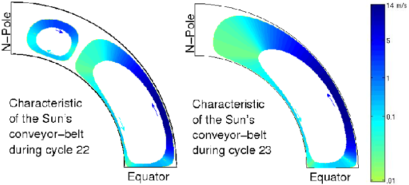
Figure 1: The Sun’s characteristic conveyor-belts during cycles 22 (left frame) and 23 (middle frame), derived from surface observations and mass-conservation, are shown. The speed associated with the colors is shown in the colorbar (right frame). The maximum surface flow-speeds at $25^{\circ}$ latitude were almost the same in both the conveyor-belts, but the flow turning down towards the equator around $60^{\circ}$ latitude during cycle 22 made the length of the primary conveyor-belt shorter than that during cycle 23, in which flow went all the way to the pole before turning equatorward.

While meridional flow at all latitudes is important for the solar dynamo, its pattern near the poles of the Sun may be particularly significant. Recently Dikpati et al (2010) showed the variation in solar cycle duration could be explained by variations in the latitudinal extent of the Sun’s primary ’conveyor belt’ or meridional circulation. Observations of the Sun’s surface Doppler plasma flow from Mount Wilson Observatory data indicate that in both cycles 22 and 23, the maximum poleward surface flow-speed in the primary belt was the same (Ulrich & Boyden (2005); also see the figure 1 of Dikpati et al (2010)). But in cycle 22, the primary circulation cell flowed poleward only to about $60^{\circ}$ latitude, thus making a shorter path for the magnetic flux transport via the conveyor belt and resulting in a cycle duration of $\sim 10.5$ years (see the left frame of Figure 1). On the other hand, in cycle 23, the poleward surface flow went all the way to the poles (see the middle frame in Figure 1), leading to a longer path via the conveyor-belt cycle of $\sim 12.5$ years.

In the past, some flux-transport dynamo calculations (Bonanno et al, 2005) and surface-transport calculations (Jiang et al, 2008) have dealt with possible multi-cell meridional flow scenarios, in the context of understanding the role of these flows in solar cycle features. We now see that these studies are not just the merely playing with models; such scenarios could happen in reality. The change in the surface poleward flow-pattern – its reversing around $60^{\circ}$ as it did in cycle 22 and maintaining poleward flow all the way to the pole as in cycle 23 – have significantly impacted the duration of cycle 23 and the length of the minimum that followed it, compared to that in cycle 22.

The plasma velocity can also be determined by helioseismic analysis, either from ring diagrams or from time-distance diagrams (Giles et al, 1997; Haber et al, 2002; Zhao & Kosovichev, 2004; Gonzalez-Hernandez et al, 2008; Gizon, Birch & Spruit, 2010). Alternatively, features seen on the images such as magnetic structures and supergranule cells, can be tracked with cross-correlation analysis to yield a drift velocity for that feature (Komm, Howard & Harvey, 1993; Snodgrass & Dailey, 1996; $\check{\rm S}$vanda et al, 2006, 2007, 2008). Ulrich (2010) reanalyzed the Mount Wilson surface Doppler data for cycles 22 and 23, from 1986 through 2009. Ulrich (2010) computed meridional flow profiles up to at least $80^{\circ}$ latitude, found smooth evolution of the signal from one year to the next, and confirmed the difference in high latitude flow patterns between cycles 22 and 23, in particular, the existence of a second reversed cell poleward of about $60^{\circ}$ during most of cycle 22, and a single cell with poleward surface flow all the way to the poles during the major part of cycle 23.

Differential rotation throughout the solar convection zone is fairly well known from helioseismic measurements (Thompson, 2004). It is difficult to measure at high latitudes because of foreshortening and other effects. Most methods measure the linear rotational velocity rather than the angular rotation rate, so it is particularly difficult to calculate the angular measure with the short moment-arm near the poles. It appears that on average the angular measure of differential rotation at the surface declines monotonically to the poles (Beck, 2000), though the existence of a ’polar vortex’ has been suggested by theory (Gilman, 1979). Although our focus on this paper is more on meridional flow at high latitudes than on differential rotation there, our model will calculate both quantities, so we will need to compare results from the model with both flows.

Given the important consequences of a second, reversed meridional cell in high latitudes, it is important to develop hydrodynamical theories that could indicate what to expect to occur in the Sun. What physics determines the presence or absense of a second cell? Can we develop a simple physical argument that we should expect to see a single primary cell, or two or more cells? This is the question we attempt to answer in this paper. The theory we develop filters out all convective instability and concentrates on forcing high latitude meridional circulation mechanically by the primary meridional flow, and possibly by differential rotation, from lower latitudes. We recognize that in the Sun there could be both this mechanical forcing and axisymmetric convection in high latitudes.

Meridional circulation is produced in virtually all fluid dynamical models used to simulate and understand the origins of the differential rotation of the Sun. These fluid dynamical models fall generally into two classes: mean field models that are axisymmetric and include parameterizations of turbulent transport of momentum (Rüdiger, 1989; Rempel, 2005), and global 3D numerical models that simulate global convection in a deep rotating spherical shell (Miesch et al, 2008). For both types of models there are numerous results that show a wide variety of meridional flow patterns, but recently both approaches have been converging toward a common result of a dominant meridional flow cell that has poleward flow near the outer boundary, and equatorward return flow near the bottom (Rempel, 2005; Miesch et al, 2008).

For some parameter choices the mean field models give a second, reversed cell at high latitudes (Rempel, 2005) and the 3D global convection models can give multiple high latitude cells (Miesch et al, 2008). Both classes of models also show that the percentage fluctuations in the amplitudes of meridional flow with time are much larger than for the differential rotation. This appears to be due to time-fluctuations in the Reynolds stresses and the fact that the meridional flow is a result of a slight imbalance between large forces, while the forces responsible for differential rotation are small enough to make the differential rotation change only very slowly.

These models are all global, and focused primarily on the problem of understanding the details of differential rotation with depth and latitude in the Sun, as well as such features as torsional oscillations. To focus primarily on the fluid dynamics of high latitudes, it is possible to build simpler models, particularly at first, and then build up to more realistic models more comparable to the global models just described. This is the approach we take below.

2 DEVELOPMENT OF THEORY

As far as is known, all main sequence stars with outer convection zones rotate, so they all have well defined equatorial planes and rotation poles. They are also almost certain to have a meridional circulation. But depending on the rotation rate, as well as the convection zone thickness, this circulation could differ greatly (Küker& Rüdiger, 2005, 2008). For example, fast-rotating solar type stars may have meridional circulation whose primary cell has flow toward the equator rather than the poles as on the Sun (Rüdiger & Küker, 2002). We know little about meridional flow from observations in stars other than the Sun, but a comparision to planetary circulations makes the point.

Most planetary atmospheres for which there are velocity measurements display meridional circulation cells, the number of which in each hemisphere varies significantly from planet to planet (due in part to the differences in planetary rotation rate) and with seasons as well as the presence or absence of internal heat sources. Jupiter is a rather fast rotator, and it has many axisymmetric meridional cells between equator and pole (see Kaspi, Flierl & Showman (2009) and references therein). By contrast, Venus, a slow rotator, has a much more global pattern of meridional flow with usually only a single cell between equator and pole (Lebonnois et al, 2010). Mars (Heavens et al, 2011) and Earth (Lorenz, 1967) have two or three cells in each hemisphere. In the Earth’s atmosphere, the so-called Hadley cell is the counterpart to the primary meridional cell in the solar convection zone. This Hadley cell, and the so-called Ferrell cell poleward of it, which is a countercell, show substantial variations in amplitude, latitudinal extent, as well as multiple equilibria in simple models (Hu, Zhou & Liu, 2011; Levine & Schneider, 2011; Adam & Paldor, 2010; Bellon & Sobel, 2010; Friersen, Lu & Chen, 2007). The driver of these circulations is different than in stars, nevertheless the observed patterns of planetary and solar circulation cells compare well.

As the Sun demonstrates, well defined meridional circulation exists and persists in the solar convection zone despite the much larger rms velocities of the convective turbulence. This turbulence, influenced by rotation, is generally thought to be the driver of the Sun’s differential rotation, and may also play a role in maintaining the meridional flow. A good place to start in considering a theory for meridional circulation is Rempel (2005), who showed that in a mean field theory of differential rotation, the buildup of higher angular velocity in equatorial latitudes leads to an outward radial Coriolis force which drives fluid up to the outer boundary from below. By mass conservation this fluid must flow toward the poles and eventually return to the bottom at higher latitudes to complete the flow circuit. What is less clear from this reasoning is to how high a latitude should the circulation reach. For flux-transport dynamos, this is a crucial question, since the period of the solar dynamo may be determined by the length of this meridional circulation ’conveyor belt’ (Dikpati et al, 2010).

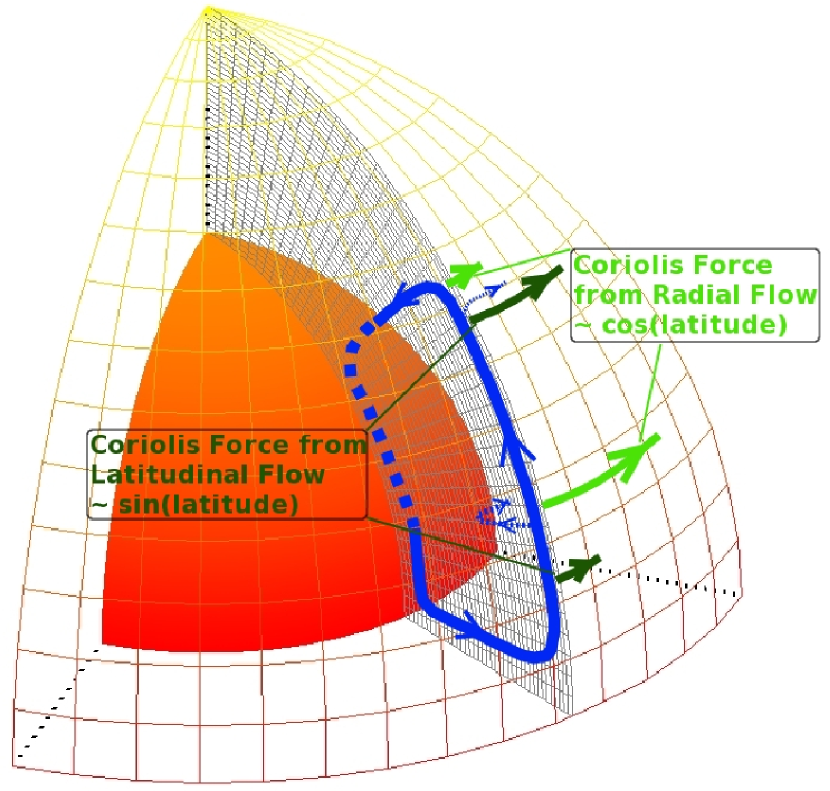
Figure 2: Schematic diagram of Coriolis forces from meridional flow as a function of latitude, illustrating that the force from radial flow is large in low latitudes and low at high latitudes, while the Coriolis force from latitudinal flow is small in low latitudes and large in high latitudes.

The radial Coriolis force may drive the meridional circulation in low and perhaps midlatitudes, but it can not do so in high latitudes, because, since there the rotation axis and the local vertical are nearly parallel, the radial Coriolis force is very weak (see Figure 2). Moreover, retaining it in the equations of motion complicates the problem mathematically. In particular, retaining the radial component of Coriolis force precludes using separation of variables to solve even the axisymmetric problem for a spherical polar cap. Therefore we will begin from the spherical shell equations but then approximate the spherical polar cap (see Figure 3) by a cylinder with the same polar axis; this eliminates the relatively mild spherical curvature in the cap while retaining the strong convergence to the pole. Then the outer boundary of the cylinder is identified with low latitude boundary of the spherical polar cap.

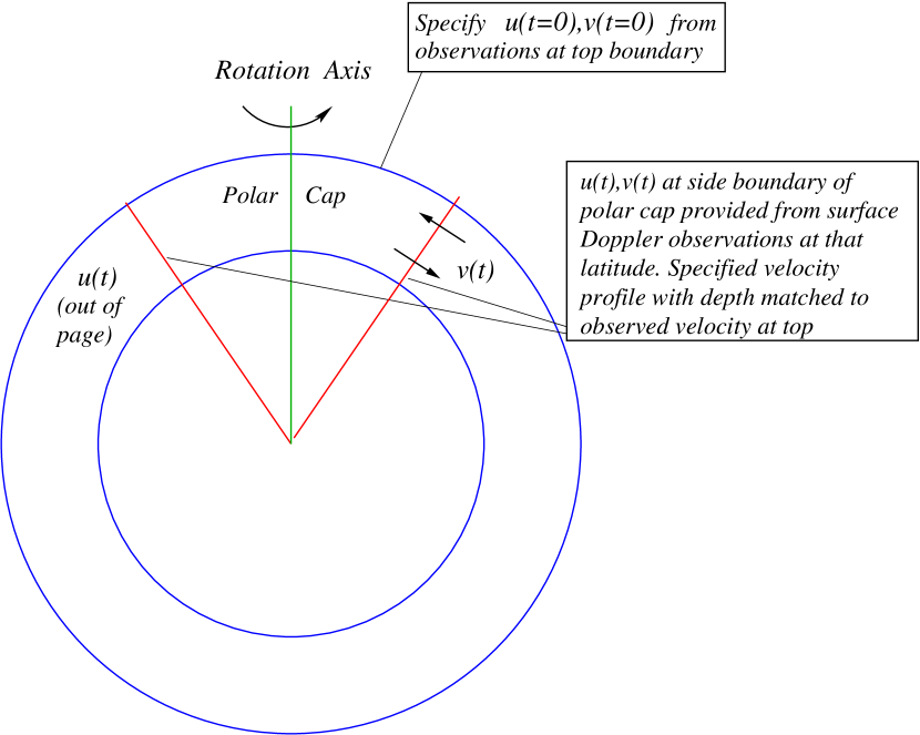
Figure 3: Schematic diagram showing our ’polar cap’ computation domain for calculating meridional flow and differential rotation. This domain is bounded in latitude by the red radial lines, and at the top and bottom boundaries of the convection zone, depicted by the concentric blue circles. For simulations of time average meridional flow and differential rotation in the polar cap, both velocities would be specified on the latitudinal boundary, guided by surface observations at that latitude. These solutions are compared to the observed surface flows at the top of the cap. For simulations of time varying flow, the model would use time dependent side boundary conditions, again taken from observations, and would initialize the integration with observations at the top boundary of the cap.

We recognize that imposing such a boundary is somewhat artificial, since no such physical boundary exists in the Sun. But we can think of it as the location where the physics that determines the meridional flow changes from the forces that are dominant in low and mid-latitudes, to those that are most important at high latitudes. We do not know exactly the latitude where the dominant forces change, so we treat the location of the boundary as a parameter of the problem. One guide to its placement comes from numerical simulations of global convection in deep rotating spherical shells (Gilman, 1979; Miesch et al, 2008) that show for a shell of the thickness of the solar convection zone as a fraction of the radius, the latitudinal Reynolds stress that transports angular momentum toward the equator to maintain the differential rotation reaches only to about $60^{\circ}$ latitude.

But even this cylindrical problem must be solved numerically; we can get a first idea of the nature of meridional flow in high latitudes by further approximating the cylinder with a cartesian analog. In this analog the cylinder is replaced by a channel infinite in longitude, whose left side boundary is identified with the axis of the cylinder, and whose right side boundary is identified with the outer wall of the cylinder. Thus through this sequence of transformations of the equations we can trace the side boundaries of the cartesian channel back to the polar axis and equatorward boundary of the spherical polar cap. This cartesian geometry allows solutions in ’latitude’ in terms of simple periodic and exponential functions. We judge that such a simplification is justified for a first study of the polarcell problem, but should be followed by much more realistic systems, which we plan for future papers.

To make this connection back to the spherical problem as strong as possible, we apply the same boundary conditions in the cartesian case as we would have in the cylindrical and spherical cases. In words, in the spherical cap case these conditions are that all physical variables remain bounded at the polar axis and axisymmetry is maintained. These requirements imply that the azimuthal flow, the latitudinal flow, the latitudinal pressure gradient and the viscous stress all vanish on the axis. To actually solve the cylindrical problem, we would apply the same conditions on the axis of the cylinder, but latitude is replaced by the cylindrical radius variable as a coordinate. In the cartesian analog, the cylindrical radius variable is replaced by the cross-channel coordinate of the infinite channel, and the azimuthal coordinate by the coordinate along the channel. In all three systems, the meridional and azimuthal flows are specified on the boundary that corresponds to the equatorward boundary of the spherical polar cap, namely the outer boundary of the cylinder, and the right hand side boundary of the channel.

In the cartesian problem, the boundary conditions at the sides introduce the possibility that momentum associated with the flow parallel to the channel walls can enter the domain from the right side and exit from the left, which has no counterpart in the cylindrical or spherical cases. But we can show that this transfer has no effect on the solutions for meridional flow, so it is not significant dynamically.

In determining meridional circulation quantitatively, the large increase in fluid density with depth in the convection zone has to be important, but it also adds considerable mathematical complexity. It is possible to write the equations of motion in terms of mass flux rather than velocities, in which case the effect of the density increase with depth is seen explicitly only in lower order terms in the turbulent diffusion expressions. We will keep these terms in the initial equations shown below, but set aside this variation in looking for the first simplest solutions.

Other effects of possible importance in determining meridional circulation in the solar convection zone include departures from the adiabatic gradient, so that buoyancy forces come into the problem, and jxB forces from magnetic fields. Departures from the adiabatic gradient, particularly their variations in latitude, could be important for determining the profile of differential rotation in the bulk of the convection zone and at its base, but the meridional flow is not very different from the case with adiabatic stratification. Therefore we will initially leave out such departures from the adiabatic. This means that when the hydrostatic pressure of the reference state is subtracted from the equations, gravity (which includes the centrifugal force of the rotating coordinate system) drops out of the problem. The effects of magnetic stresses are also deferred to a later paper. Because meridional flow and differential rotation are very subsonic flows, we do not expect acoustic effects to be important, so we start from equations in which acoustic modes have been filtered out. In that case the mass-continuity equation contains no time derivative. We are in effect using the so-called ’anelastic’ equations.

3 MATHEMATICAL FORMULATION

In this section we develop the hierarchy of equations for meridional circulation and differential rotation in the polar cap, starting from vector-invariant forms of the equations of motion and mass conservation.

3.1 Vector invariant and spherical component equations

In vector form, the equations of motion are given by

$${\partial{{\mathbf{v}}}\over\partial t}=-{1\over\rho}\mbox{\boldmath$\nabla$}p-\mbox{\boldmath$\nabla$}\left({\mathbf{v}}\cdot{\mathbf{v}}/2\right)+{\mathbf{v}}{\mathbf{\times}}\left(\mbox{\boldmath$\nabla$}{\mathbf{\times}}{\mathbf{v}}\right)-2{\Omega}{\mathbf{\times}}{\mathbf{v}}-{1\over\rho}\mbox{\boldmath$\nabla$}{\mathbf{\times}}\rho\nu\left(\mbox{\boldmath$\nabla$}{\mathbf{\times}}{\mathbf{v}}\right)-g\hat{z}\quad$$

and

$$\mbox{\boldmath$\nabla$}{\mathbf{\cdot}}\hskip 1.5pt\left(\rho{\mathbf{v}}\right)=0.\quad$$

If we subtract out a reference state hydrostatic balance, then gravity is removed from the problem and the pressure variable $p$ contains the departure of pressure from this hydrostatic balance. In this anelastic system, the density $\rho$ is the reference state density. Then in spherical coordinates ($r,\theta,\phi$) the component equations for the flow are

$${\partial w\over\partial t}=-{1\over\rho}{\partial p\over\partial r}+2\Omega\sin\theta u-{1\over{\rho r^{2}\sin\theta}}{\partial\over\partial\theta}\left(\rho\nu\sin\theta\left({\partial\over\partial r}(rv)-{\partial w\over\partial\theta}\right)\right)+F_{r};\quad$$

$${\partial v\over\partial t}=-{1\over\rho r}{\partial p\over\partial\theta}+2\Omega\cos\theta u+{1\over\rho r}{\partial\over\partial r}\left(\rho\nu\left({\partial\over\partial r}(rv)-{\partial w\over\partial\theta}\right)\right)+F_{\theta};\quad$$

$${\partial u\over\partial t}=-2\Omega\cos\theta v-2\Omega\sin\theta w+{1\over\rho r}\left({\partial\over\partial r}\left(\rho\nu{\partial\over\partial r}(ru)\right)+{1\over r}{\partial\over\partial\theta}\left({\rho\nu\over\sin\theta}{\partial\over\partial\theta}\left(\sin\theta u\right)\right)\right)+F_{\phi}.\quad$$

These equations are subject to the constraint of mass-conservation, given by

$${1\over r}{\partial\over\partial r}(\rho r^{2}w)+{1\over\sin\theta}{\partial\over\partial\theta}(\rho\sin\theta v)=0.\quad$$

In these equations, $u$ is the (linear) rotational velocity, $v$ the velocity in colatitude $\theta$ and $w$ the radial velocity. $\Omega$ is the rotation rate of the coordinate system, $\rho$ the reference state density, which varies only in radius, $p$ the pressure relative to a spherically symmetric hydrostatic pressure, $\nu$ the turbulent viscosity. $F_{r},F_{\theta}$ and $F_{\phi}$ are force components that would arise from turbulent Reynolds stresses. Nonlinear inertial terms involving products of axisymmetric meridional and rotational flow have been excluded from equations for simplicity and because the turbulent Reynolds stresses should be larger. A nonzero $F_{\phi}$ in the polar cap leads to ‘gyroscopic pumping’ as described in McIntyre (2007). In particular, if this process is at work, in order to get poleward flow the Reynolds stress must be transporting angular momentum toward the equator there, by an amount that increases with colatitude.

3.2 Spherical equations for streamfunction and rotational velocity

Equations (3)-(6) above can be solved as is, or the perturbation pressure can be eliminated by cross-differentiation of equations (3) and (4), together with defining a streamfunction $\chi$ for the meridional flow $v,w$ such that the mass continuity equation (6) is satisfied automatically. By inspection, this streamfunction is defined so that

$$\rho w={1\over r\sin\theta}{\partial\over\partial\theta}(\sin\theta\chi);\rho v=-{1\over r}{\partial\over\partial r}(r\chi).\quad$$

The prediction equation for $\chi$ is given by

$${\partial\over\partial t}L\chi=-{2\Omega\cos\theta\over r}{\partial\over\partial r}(r\rho u)+{2\Omega\over r}{\partial\over\partial\theta}(\sin\theta\rho u)$$

$$+L(\nu L\chi)-L\left({\nu\over r}{\partial(ln\rho)\over\partial r}{\partial\over\partial r}(r\chi)\right)$$

$$-{1\over r}{\partial\over\partial r}(\rho rF_{\theta})+{\rho\over r}{\partial\over\partial\theta}F_{r},\quad$$

in which the $L\chi$ is defined by

$$L\chi=\left(\nabla^{2}-{1\over r^{2}\sin^{2}\theta}\right)\chi.\quad$$

Here $\nabla^{2}$ is the standard axisymmetric Laplacian operator in spherical polar coordinates.

Finally the prediction equation (5) for the rotational flow $u$ becomes

$${\partial\over\partial t}u={2\Omega\cos\theta\over\rho r}{\partial\over\partial r}(r\chi)-{2\Omega\over\rho r}{\partial\over\partial\theta}(\sin\theta\chi)+{1\over\rho r}{\partial\over\partial r}(\rho\nu{\partial\over\partial r}(ru))+{1\over\rho r^{2}}{\partial\over\partial\theta}({\rho\nu\over\sin\theta}{\partial\over\partial\theta}(\sin\theta u))+F_{\phi}.\quad$$

Equations (8)-(10) can be solved numerically. However, this is the first attempt to understand the flow behavior in the Sun’s polar latitudes. So, in order to understand how this model works, we seek further approximations to a cylindrical system as an intermediate step before going to a rectangular system.

3.3 Cylindrical component equations

In this subsection, we define a cylindrical coordinate system whose axis coincides with the rotation axis of the Sun. The independent variables in this system are $s,\phi,z$; $s$ is the outward radial coordinate (colatitude at the pole), $\phi$ the azimuthal coordinate (longitude on the Sun), and $z$ the axial coordinate (corresponding to the outward radial coordinate at the pole). The corresponding velocities for these coordinates are defined as $v,u,w$. If we restrict ourselves to axisymmetric variables, then the azimuthal flow $u$ is identified with the solar differential rotation linear velocity in high latitudes, and $v,w$ with the solar meridional circulation there. In the axisymmetric case, the three component equations of fluid motion are given by,

$${\partial v\over\partial t}=-{1\over\rho}{\partial p\over\partial s}-{\partial\over\partial s}\left({v^{2}+u^{2}+w^{2}\over 2}\right)+{u\over s}{\partial\over\partial s}\left(su\right)+w\left({\partial w\over\partial s}-{\partial v\over\partial z}\right)$$

$$+2\Omega u-{1\over{{\rho}s}}{\partial\over\partial z}\left(s\rho\nu\left({\partial w\over\partial s}-{\partial v\over\partial z}\right)\right);\quad$$

$${\partial u\over\partial t}=-{v\over s}{\partial\over\partial s}(su)-w{\partial\over\partial z}(su)-2\Omega v+{1\over\rho}{\partial\over\partial s}\left({\rho\nu\over s}{\partial\over\partial s}(su)\right)+{1\over\rho}{\partial\over\partial z}\left({\rho\nu\over s}{\partial\over\partial z}(su)\right);\quad$$

$${\partial w\over\partial t}=-{1\over\rho}{\partial p\over\partial z}-{\partial\over\partial z}\left({v^{2}+u^{2}+w^{2}\over 2}\right)+u{\partial\over\partial z}(su)-v\left({\partial w\over\partial s}-{\partial v\over\partial z}\right)$$

$$+{1\over\rho s}{\partial\over\partial s}\left(s\rho\nu\left({\partial w\over\partial s}-{\partial v\over\partial z}\right)\right).\quad$$

In cylindrical coordinates the axially symmetric mass continuity equation is given by,

$${1\over s}{\partial\over\partial s}(\rho sv)+{\partial\over\partial z}(\rho w)=0.\quad$$

3.4 Steady state linear equations

The simplest meaningful problem we can solve is one in which the flow is taken to be steady and the velocities relative to the rotating reference frame are small enough that the nonlinear inertial terms can be dropped. We also take $\rho$ and $\nu$ to be independent of $s$ and functions only of $z$. The fluid flow inside the cylinder is forced by fluid entering and leaving from the outer radial boundary (the equivalent of a latitude circle in the spherical case).

With the above conditions, the mass continuity equation (14) is unchanged, while the equations of motion (11)-(13) reduce to

$${1\over\rho}{\partial\over\partial z}\left(\rho\nu\left({\partial w\over\partial s}-{\partial v\over\partial z}\right)\right)+{1\over\rho}{\partial p\over\partial s}-2\Omega u=0;\quad$$

$$\nu{\partial\over\partial s}\left({1\over s}{\partial\over\partial s}(su)\right)+{1\over\rho}{\partial\over\partial z}\left(\rho\nu{\partial u\over\partial z}\right)-2\Omega v=0;\quad$$

$${\nu\over s}{\partial\over\partial s}\left(s\left({\partial w\over\partial s}-{\partial v\over\partial z}\right)\right)-{1\over\rho}{\partial p\over\partial z}=0.\quad$$

The physical boundary conditions we take for the cylinder are to allow no flow through, and no viscous stress on, the top and bottom; we impose meridional flow on the outer radial boundary, representing the primary poleward cell in the Sun. To obtain steady solutions, there must also be no net torque applied to the outer boundary. As stated above, certain conditions must also be imposed on the axis, to ensure all physical variables remain bounded and single-valued there and axisymmetry is maintained. These requirements imply that azimuthal flow $u$, radial flow $v$, radial pressure gradient and viscous stress all vanish there.

3.5 Separation of variables: incompressibile case

3.5.1 Separated equations

If we discard density variations in the $z$ direction, so density is constant, we can absorb the density into the pressure, defining a new variable $\Pi$=$p/\rho$. Then we define a stream function $\psi$ that satisfies the mass continuity equation through the relations

$$v=-{\partial\psi\over\partial z};w={1\over s}{\partial\over\partial s}(s\psi).\quad$$

With these variable changes, equations (15)-(17) become

$$\nu{\partial\over\partial z}\left(\nabla^{2}\psi-\psi/s^{2}\right)-2\Omega u+{\partial\Pi\over\partial s}=0;\quad$$

$$\nu\nabla^{2}u+2\Omega{\partial\psi\over\partial z}=0;\quad$$

$${\nu\over s}{\partial\over\partial s}\left(s(\nabla^{2}\psi-\psi/s^{2})\right)-{\partial\Pi\over\partial z}=0.\quad$$

In equations (19)-(21), $\nabla^{2}$ is the standard axisymmetric cylindrical Laplacian operator.

We can eliminate the pressure variable $\Pi$ from equations (19) and (21) by cross differentiation, reducing the system to one second order equation, equation (20), and one fourth order equation, given by

$$\left(\left(\nabla^{2}-1/s^{2}\right)\left(\nabla^{2}\psi-\psi/s^{2}\right)\right)-2\Omega{\partial u\over\partial z}=0.\quad$$

There are two distinct classes of solutions to the system (20),(22). Since these equations are linear, these solutions can be superimposed with relative amplitudes determined by the boundary conditions for each. One class is found by setting the meridional flow streamfunction $\psi=0$ everywhere. It yields pure differential rotation independent of $z$ forced at the outer boundary of the cylinder. To satisfy the condition that there be no net torque at the outer boundary, to allow steady solutions in the interior of the cyclinder, there must be no viscous stress at this boundary. This corresponds to solutions with constant angular velocity, or linear rotational velocity $u$ that decreases linearly with $s$ toward the axis of the cylinder. The other class of solutions can be found by separation of variables, since coefficients in this system are functions of $s$ only. We place the lower and upper boundaries of our cylinder at $z=0,H$ respectively. Then if we allow no flow through the lower or upper boundary, these boundaries must coincide with a streamline, and there should be no viscous stress there either. These conditions are satisfied if we take

$$\psi=\sum_{n=1}^{\infty}\Psi_{n}\sin(n\pi z/H);u=\sum_{n=1}^{\infty}U_{n}\cos(n\pi z/H).\quad$$

With this choice of representation of the solutions, we can find separate solutions for each $n$ for $\psi$ and $u$. We can then represent the forcing at the boundary in the same way, so the amplitude of the solutions for each $n$ is determined separately by the amplitude of the forcing for the same $n$. There could be other solutions that use other representations, but we have not looked for them.

Then if we substitute expressions (23) into equations (20),(22), and define $\sigma_{n}=n\pi/H$, then equations (20) and (22) become, for each $n$,

$$\nu{{\nabla}^{2}}_{n}U_{n}+2\Omega\sigma_{n}\Psi_{n}=0,\quad$$

and

$$\nu(\left(\nabla_{n}^{2}-1/s^{2}\right)\left(\nabla_{n}^{2}\Psi_{n}-\Psi_{n}/s^{2}\right)-2\Omega\sigma_{n}U_{n}=0,\quad$$

in which

$$\nabla_{n}^{2}={1\over s}{d\over ds}s{d\over ds}-\sigma_{n}^{2}.\quad$$

The set of solutions to equations for which there is no meridional flow are for $u$ only, which from equation (22) must satisfy the relation ${\partial u\over\partial z}=0$ everywhere, so $u$ is a function of $s$ only; $u$ is independent of $z$. For $\psi=0$ everywhere, equation (20) becomes ${\partial\over\partial s}(s{\partial u\over\partial s})=0$. The solutions to this equation all are for constant angular velocity, or linear rotational velocity that is a linear function of $s$. Since this linear velocity is independent of $z$ it will also satisfy stress free boundary conditions at top and bottom. But since $\psi=0$ in these solutions, they do not contribute to determining the amplitude of meridional flow or where the nodes in this flow occur. These properties are determined entirely from solutions to equations (24)-(26) for $\Psi_{n}$ and $U_{n}$. The solutions for $u$ with $\psi=0$ everywhere can be used to match the total solution for differential rotation linear velocity with observational estimates. These total solutions will therefore have a differential rotation that is in part independent of $z$ and in part a cosine function of $z$.

3.5.2 Nodimensionalization and setting of parameters

If we scale all lengths in the problem by $H$, the depth of the cylinder, and recognize that $U_{n}$ scales differently from that of $\Psi_{n}$ by $H$, then the dimensional system (24)-(25) can be written in dimensionless form as

$$\nabla_{n}^{2}U_{n}+\epsilon_{n}\Psi_{n}=0,\quad$$

and

$$\left(\nabla_{n}^{2}-1/s^{2}\right)^{2}\Psi_{n}-\epsilon_{n}U_{n}=0,\quad$$

in which $\epsilon_{n}$ is a dimensionless parameter, defined as $\epsilon_{n}=2\Omega\sigma_{n}H^{3}/\nu$. In this dimensionless system, velocities are scaled by $\nu/H$ and therefore the streamfunction by $\nu$.

For this system the boundary conditions, defined physically in section 3.3, that should be applied are that

$$\Psi_{n}=0;\,\,{d^{2}\Psi_{n}\over ds^{2}}=0;\,\,U_{n}=0;\,\,{dU_{n}\over ds}=0\,\,\,{\rm at}\,\,\,s=0;\quad$$

and

$$\Psi_{n}\,\,{\rm and}\,\,U_{n}\,\,\,{\rm specified\,\,\,at}\,\,\,s=R.\quad$$

These boundary conditions completely specify the system for solutions containing both meridional flow and differential rotation for which $n\geq 1$. For forcing with any $n$ imposed on the boundary, there will be a response in meridional circulation and differential rotation in the interior that contains the same $n$. Since the problem is linear, solutions with multiple $n$ values can be constructed simply by adding together solutions for each individual $n$. The relative amplitudes of each of these solutions would be determined by the relative amplitudes of the forcing for different $n$.

If equations (27) and (28) were combined into a single equation for $\Psi_{n}$, it would be sixth order, yielding a total of six independent solutions. We would need to apply a total of six boundary conditions; these include four on the $z$ axis, and two at the outer radial boundary. For any added differential rotation component $U_{0}$ that satisfies the equation $d(s(dU_{0}/ds))/ds=0$ the boundary conditions are $U_{0}=0$ and $dU_{0}/ds=0$ at $s=0$, and $U_{0}$ specified at $s=R$.

$\epsilon_{n}$ is the only dimensionless parameter that is explicit in the equation system (27)-(29), but in fact there are others, implied or implicit in this system, which may be useful in evaluating the results. We define them here, and discuss their possible significance.

A traditional dimensionless number used to characterize the relative influence of Coriolis and viscous forces in a fluid dynamical problem is the so-called Taylor number $Ta=4\Omega^{2}H^{4}/\nu^{2}$. By inspection, it is related to $\epsilon_{n}$ by the relationship $\epsilon_{n}=n\pi{Ta}^{1/2}$. In a typical problem involving both rotation and viscosity, $Ta$ needs to be $10^{3}$ or higher to show substantial influence of rotation. If we take $\nu\sim 10^{12}{\rm cm}^{2}\,{\rm s}^{-1}$, $Ta=4\times 10^{6}$ for the whole depth of the solar convection zone, so we should expect a substantial influence of rotation on the solutions of most interest for the Sun. Another number often used in such problems is the Ekman number $E=1/2Ta^{1/2}$. This number would be small for the solar convection zone; it measures the thickness of the boundary layers that would form if the top or bottom of the convection zone were considered to be ’nonslip’. But, more realisticly, we take these boundaries to be stress free, so no Ekman layers are allowed to form.

Because the rotational velocity $U$ is specified on the outer boundary of the cylinder, we can also define a Rossby number $Ro=U/2\Omega H$ and a Reynolds number $Re=UH/\nu$. A plausible linear rotational velocity at the outer boundary would be $60{\rm m}\,{\rm s}^{-1}$, for which $Ro=0.115$. When $Ro<<1$ the flow tends to be geostrophic; that is, there is a near balance in latitude (radius in the cylinder) between Coriolis and pressure gradient forces. This balance should therefore be checked in the solutions we find. With the scaling we have used, the Reynolds number is the velocity itself. We should expect different behavior of the solutions depending on whether $Re>>1$ or $Re<<1$. We will see that we can get $Re>>1$ in our model only if we assume quite low turbulent viscosity $\nu\sim 10^{10}{\rm cm}^{2}\,{\rm s}^{-1}$. For most of the parameter space of interest $Re<1$, in many cases much less. In general, the implication of small $Re$ is that the flows are likely to be smooth and laminar, i.e., not turbulent. If the flow imposed at the low latitude boundary of the polar cap (outer boundary of the cylinder) is time dependent, the interior flows induced will also be, but will generally have similar time dependence to that seen at the boundary.

3.6 Formulation in cartesian geometry

3.6.1 Equations

We can get a preliminary idea of the nature of the solutions for meridional circulation and differential rotation in the cylindrical problem if we look at it in a ’cartesian limit’, found by conceptually replacing the full cylinder by a cylindrical annulus and taking both the inner and outer boundaries of the annulus to a large distance from the axis. Then all curvature effects can be ignored; a disadvantage is that we lose the convergence of the meridional flow to the polar axis. The effect of this approximation will need to be assessed in a later study. In this cartesian limit, equations (27) and (28) reduce to

$$\left({d^{2}\over dx^{2}}-\sigma_{n}^{2}\right)U_{n}+\epsilon_{n}\Psi_{n}=0\quad$$

and

$$\left({d^{2}\over dx^{2}}-\sigma_{n}^{2}\right)^{2}\Psi_{n}-\epsilon_{n}U_{n}=0,\quad$$

in which we have replaced $s$ with $x$ as the independent variable to avoid confusion between cylindrical and cartesian coordinates. Here the quantity $\sigma_{n}=n\pi$ is the dimensionless form.

Equations (30) and (31) admit of solutions of the form

$$\left(\Psi_{n},U_{n}\right)\sim e^{k_{n}x},\quad$$

in which $k_{n}$ is in general complex. Substitution of the forms (32) into equations (30) and (31) yields a $3\times 3$ determinant of the coefficients, which must vanish for there to be a nontrivial solution to the equations. This yields the relationship

$$\left(k_{n}^{2}-n^{2}\pi^{2}\right)^{3}+\epsilon_{n}^{2}=0.\quad$$

This equation has six distinct roots in $k_{n}$ for each $n$; they come in two sets of three, from

$$k_{n}=\pm\left(n^{2}\pi^{2}+(-1)^{1/3}\epsilon_{n}^{2/3}\right)^{1/2}.\quad$$

The argument of the square root has three distinct values, because $-1=e^{\pm i\pi},e^{\pm 3i\pi}$ and therefore $(-1)^{1/3}=e^{\pm i\pi/3},-1$. The first two choices yield complex $k_{n}$, meaning that these solutions are both exponential and sinusoidal with respect to $x$, while the third choice leads to $k_{n}$ either real or imaginary, depending on the values of $n$ and $\epsilon_{n}$. These solutions are therefore either purely exponential or purely oscillatory with respect to $x$. In general, we expect to need all six solutions for $k_{np},p=1,6$ to satisfy the boundary conditions at the sides of the Cartesian channel.

As stated above, the left hand edge of the cartesian channel corresponds to the axis in cylindrical geometry. In the cylindrical case we required $U_{n}=0$ on the axis, to keep the angular velocity finite and avoid multiple-valued functions, but, strictly speaking, these conditions do not apply in the cartesian case. However, for comparison with the cylindrical and spherical systems, we retain the same boundary conditions. This has the artificial effect of allowing momentum to cross this boundary, which can not happen in the cylindrical or spherical cases. But this property is inconsequential in that it has no effect on the solutions for meridional circulation.

In the cartesian limit we have distorted only the geometry in order to find analytical solutions that should tell us something about how extended the primary meridional flow cell is as a function of the parameters of the problem, particularly $\epsilon_{n}$, which is the same in cartesian and cylindrical cases. Therefore in cartesian coordinates the boundary conditions are

$$\Psi_{n}=0,{d^{2}\Psi_{n}\over d^{2}x}=0,U_{n}=0,{dU_{n}\over dx}=0,\,\,\,{\rm at}\,\,\,x=0;\quad\Psi_{n},U_{n}\,\,\,{\rm specified\,\,at}\,\,\,x=R.\quad$$

Next we generalize the equation forms (32) to account for the six solutions for each variable by representing each as

$$\Psi_{n}=\sum_{p=1}^{6}\Psi_{np}e^{k_{np}x},\quad U_{n}=\sum_{p=1}^{6}U_{np}e^{k_{np}x}.\quad$$

Then satisfaction of the boundary conditions at $x=0$ requires that

$$\sum_{p=1}^{6}\Psi_{np}=0,\quad\sum_{p=1}^{6}k_{np}^{2}\Psi_{np}=0,\quad\sum_{p=1}^{6}U_{np}=0,\quad\sum_{p=1}^{6}k_{np}U_{np}=0.\quad$$

Satisfaction of the inhomogeneous boundary conditions at the right hand boundary of the channel (corresponding to the outer radial boundary of the cylinder) requires

$$\sum_{p=1}^{6}\Psi_{np}e^{k_{np}R}=\Psi_{n}(R),\quad\sum_{p=1}^{6}U_{np}e^{k_{np}R}=U_{n}(R),\quad$$

in which $\Psi_{n}(R)$ and $U_{n}(R)$ are the values imposed on the system by the boundary conditions at the right hand boundary $x=R$.

Then equations (37) and (38) are a system of six linear equations, four homogeneous, two inhomogeneous, for 12 independent variables – seemingly a very underdetermined system. But we must recognize that equations (30)-(31) impose relationships among $\Psi_{np},U_{np}$, since they all must be satisfied separately for each $n,p$. These relationships are

$$(k_{np}^{2}-\sigma_{n}^{2})U_{np}+\epsilon_{n}\Psi_{np}=0;\quad\quad p=1,6\quad$$

and

$$(k_{np}^{2}-\sigma_{n}^{2})^{2}\Psi_{np}-\epsilon_{n}U_{np}=0;\quad\quad p=1,6.\quad$$

If we invoke all these relationships, then it would seem that the system is overdetermined, but since the $k_{np}$ are found from equation (33) also by substitution of form (32) into (30)-(31) only one of equations (39)-(40) are in fact independent. Therefore (39)-(40) provide twelve independent relationships among $\Psi_{np}$ and $U_{np}$, exactly what we need to constrain and solve the system (37)-(38) for these variables. In practice, we eliminate $U_{np}$ from (37) and (38) by substitution from (39). These equations are:

$$\sum_{p=1}^{6}\Psi_{np}=0;\quad$$

$$\sum_{p=1}^{6}{k_{np}^{2}}\Psi_{np}=0;\quad$$

$$\sum_{p=1}^{6}{1\over(k_{np}^{2}-\sigma_{n}^{2})}\Psi_{np}=0;\quad$$

$$\sum_{p=1}^{6}{k_{np}\over(k_{np}^{2}-\sigma_{n}^{2})}\Psi_{np}=0;\quad$$

$$\sum_{p=1}^{6}e^{k_{np}R}\Psi_{np}=\Psi_{n}(R);\quad$$

and

$$\sum_{p=1}^{6}{\epsilon_{n}e^{k_{np}R}\over(k_{np}^{2}-\sigma_{n}^{2})}\Psi_{np}=-U_{n}(R).\quad$$

These equations can be solved using Cramer’s rule, provided the $6\times 6$ determinant of the coefficients of these equations does not vanish. This system has either one or two inhomogeneous equations, and respectively either five or four homogeneous equations.

By separating the real and imaginary parts of these six complex equations, we numerically solve the system of twelve linear equations by factoring into lower and upper triangular form followed by back substitution. The magnitudes of solution vectors varies widely in the range of parameters of our interest. However, we have found that it is always the case that the highest magnitude of $L^{2}=||{\bf A}\cdot{\bf x}-{\bf b}||$ norm error of the solved system is at least twelve orders of magnitude lower than the magnitudes of solution vectors.

If we wish to add to these a solution for pure differential rotation (no meridional flow) driven by a linear rotation velocity independent of $z$ on the right hand channel boundary, it must satisfy the relationship $d^{2}U_{0}/d^{2}x=0$ with $U_{0}=0$ at $x=0$ and $U_{0}$ specified at the right hand boundary, so this flow simply decreases linearly to zero from right to left, corresponding to constant angular velocity in the cyclindrical and spherical cases. Not surprisingly, in the cartesian case, it is not possible to satisfy the boundary condition $dU_{0}/dx=0$ at $x=0$, because momentum that flows in from the right side must flow out on the left side to maintain a steady state. As stated above for the cylindrical case, these linear solutions have no effect on the amplitudes or the positions of the nodes in $x$ for meridional flow or differential rotation that are functions of $z$.

3.6.2 Parameter ranges of interest

There are four independent parameters to be varied in our dimensionless cartesian system. These include $\epsilon_{n}$, which measures the relative influence of Coriolis and viscous forces; $R$, which measures the aspect ratio of the channel and therefore the colatitude of the equatorial boundary of the polar cap; $U_{n}(R)$, the linear rotational velocity imposed at this boundary; and $\Psi_{n}(R)$, representing the meridional flow imposed there. To estimate the range of $\epsilon_{n}$ of interest, we use for $\Omega$ the core rotation rate of the Sun, $2.6\times 10^{-6}{\rm s}^{-1}$ and for $H$ the depth of the convection zone, $2\times 10^{10}{\rm cm}$. Then the range of $\epsilon_{n}$ is given by $6.53\times 10^{15}n/\nu$. Therefore for the range $10^{11}<\nu<10^{16}{\rm cm}^{2}\,{\rm s}^{-1}$ for $n=1$, the lowest vertical mode, we get $6.53\times 10^{4}>\epsilon_{1}>0.653$. The most plausible values for $\nu$ in the convection zone of the Sun are in the range $10^{12}-10^{14}{\rm cm}^{2}\,{\rm s}^{-1}$.

A typical dimensional meridional flow speed observed in midlatitudes near the boundary of our polar cap falls in the range -5 to -20 ${\rm m}\,{\rm s}^{-1}$ (the negative sign is for flow toward the left hand edge of the channel, corresponding to poleward flow in the polar cap). Relative to the core rotation rate, a surface linear rotational flow speed at similar latitudes would be in the range -20 to -90 ${\rm m}\,{\rm s}^{-1}$. What dimensionless values these correspond to vary according to what value of $\nu$ we assume. For $5\,{\rm m}\,{\rm s}^{-1}$ and $\nu$ of $10^{11}\,{\rm cm}^{2}\,{\rm s}^{-1}$ we get a dimensionless velocity of one unit and a streamfunction of $1/\pi$ units. For a dimensional speed of $90\,{\rm m}\,{\rm s}^{-1}$ and $\nu$ of $10^{15}{\rm cm}^{2}\,{\rm s}^{-1}$, the dimensionless velocity is $1.8\times 10^{-4}$ units. The streamfunction associated with a peak meridional flow of $20\,{\rm m}{\rm s}^{-1}$ and $\nu=10^{15}\,{\rm cm}^{2}\,{\rm s}^{-1}$ is $4\times 10^{-4}/\pi$. The results that follow will be for parameter values within these ranges and for even higher viscosity, in order to show the full range of behavior of the solution with respect to node number and location.

In the case of the differential rotation linear velocity imposed at the side boundary, we must decide the relative amplitudes of the $z$ independent part $U_{0}$ and the $z$-dependent part $U_{n}$. This choice will be guided by observations. Whatever the choice, only the $z$ dependent part of $U$ has dynamical consequences for the meridional flow and the position of its nodes.

4 RESULTS

Our results are of two types: displays of the latitude positions of all the nodes in the streamfunction as functions of the parameters of the problem, and contour plots of that streamfunction. We discuss node position first. We focus on solutions for which the boundary forcing is chosen with $n=1$, corresponding to a primary meridional circulation cell that has poleward flow in the upper half of the polar cap, and equatorward flow in the lower half. To produce a meridional flow in the polar cap that contains $n>1$ requires forcing at the boundary that includes components with $n>1$, which, if the amplitude of the $n>1$ components were large enough, would imply the existence of more than one meridional flow cell with depth at all latitudes, as well as latitudinal differential rotation changing sign with depth. We are not aware of observational evidence for such flows, so we have not considered that case. We could alter the simple $\sin\pi z$ dependence with depth without introducing a second cell, if we added a $\sin 2\pi z$ term to the forcing with a sufficiently small amplitude factor. We have not explored that possibility in this paper.

4.1 Latitude locations of nodes

Figure 4 displays the latitude positions of streamfunction nodes for a solar type turbulent viscosity of $\nu=10^{13}{\rm cm}^{2}\,{\rm s}^{-1}$ for a range of plausible meridional flows and four choices of differential rotation imposed at the boundary, which for this case is at $60^{\circ}$ latitude. Figure 5 displays node position as a function of boundary meridional flow speed for boundaries set at $60^{\circ}$, $65^{\circ}$ and $70^{\circ}$ (frames a,b,c respectively), for a wide range of turbulent viscosities and for a plausible rotation of the solar core. We recognize that the range of viscosities is much wider than plausible for the sun, but in this first study we want to illustrate the full range of behavior of our model. Figure 6 illustrates detailed behavior of the nodes for the boundary at $65^{\circ}$ in a part of the parameter space in which a change in the meridional flow at the boundary leads to a merging of nodes, which implies that the number of nodes drops from two to zero. Figure 7 displays the latitude of the first and second nodes as functions of the turbulent viscosity for the different boundary placements and a typical flow speed, namely $10\,{\rm m}\,{\rm s}^{-1}$.

Figure 4 shows that for the parameters chosen there are two nodes within the channel, the first located between $60^{\circ}$ and $65^{\circ}$ (solid color curves), the second between $76^{\circ}$ and $81^{\circ}$ (dashed curves), depending on the meridional flow amplitude at the boundary. The red curves are for a vertical and latitudinal differential rotation linear velocity that approximates the solar profile at $60^{\circ}$; hence the label ’Normal’. The other curves are for specified fractions of that value. We see from Figure 4 that the latitude of nodes is only weakly a function of differential rotation at the boundary, so in subsequent results presented we focus on a solar differential rotation. We do this also because we know from helioseismic measurements that the differential rotation profile changes very little with time (torsional oscillations are only a few % of the time average differential rotation). In addition, the latitude spacing between the first and second nodes, about $16^{\circ})$, is virtually independent of choice of differential rotation and meridional flow speed.

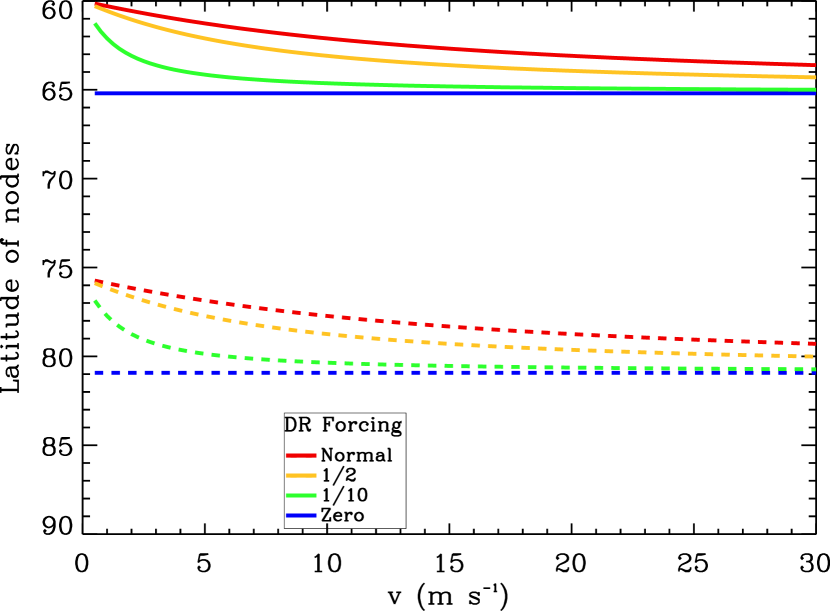
Figure 4: Latitudinal positions of streamfunction nodes as a function of meridional flow speed at the boundary, for selected differential rotation amplitudes at the same boundary (color key is shown in the figure).

How sensitive are the node positions to the turbulent viscosity? Figure 5 gives the answer. For all three boundary latitudes, for $\nu=10^{12}{\rm cm}^{2}\,{\rm s}^{-1}$, there are three nodes. For $10^{13}{\rm cm}^{2}\,{\rm s}^{-1}$ there are two. For $\nu=10^{15}$ and above there is at most one node; as the turbulent viscosity is raised, the range of meridional flow speeds for which there is even one node shrinks toward zero. For meridional flow speeds at the boundary of, say, $10\,{\rm m}\,{\rm s}^{-1}$, the last node does not disappear until the turbulent viscosity is as high as $10^{16}-10^{17}{\rm cm}^{2}\,{\rm s}^{-1}$, values two to three orders of magnitude larger than plausible for the Sun, even for the solar surface where supergranules are active.

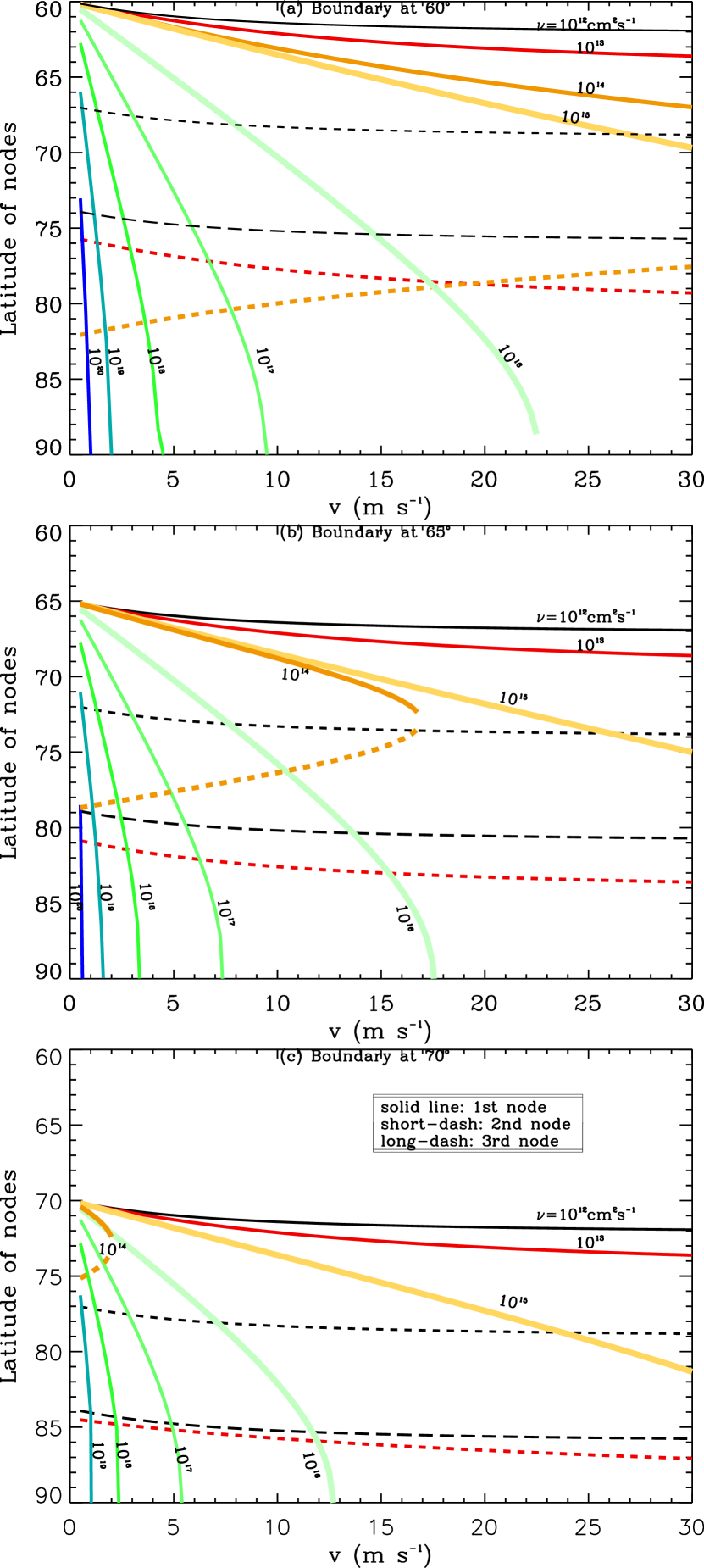
Figure 5: Latitudinal positions of streamfunction nodes as a function of meridional flow speed at the boundary, for solar type differential rotation amplitude at the same boundary and a wide range of values of turbulent viscosity, for boundaries at $60^{\circ}$ (frame a), $65^{\circ}$ (frame b) and $70^{\circ}$ (frame c). Solid curves are for the location of the node closest to the imposed boundary, short dashed curves the second node, and long dashes the third node. The color code is defined by the viscosity values shown on each of the solid curves.

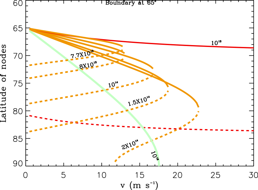
Figure 6: Latitudinal positions of streamfunction node for boundary at $65^{\circ}$ as a function of meridional flow speed, for turbulent viscosities for which an increase of meridional flow speed leads to node merger. The color code is defined by the curve labels.

We might conclude from these results that it is virtually impossible to generate meridional flow that reaches all the way to the pole for solar like viscosity, and that therefore some additional physics would be necessary to include to create such flow for solar conditions. But this conclusion would be premature, since in frames 5b and c we see evidence of node ’merging’ as the meridional flow is increased. Two nodes merge, eliminating both at higher meridional flow speeds. This occurs near $\nu=10^{14}{\rm cm}^{2}\,{\rm s}^{-1}$ (see orange solid and dashed curves). For the boundary at $65^{\circ}$ this merger takes place at a meridional flow speed of about $17{\rm m}\,{\rm s}^{-1}$, and for a boundary at $70^{\circ}$, at about $2{\rm m}\,{\rm s}^{-1}$. Other neighboring boundary placements would yield merger flow speeds near these values. We show streamfunctions for parameter values near those for which merger occurs in the next section.

Figure 6 gives a more detailed picture of the range of parameter values for which node merger occurs. Here we display node latitudes for several turbulent viscosity values in the range $10^{13}-10^{16}{\rm cm}^{2}\,{\rm s}^{-1}$. We see that from $\nu=7.7\times 10^{13}$ up to $2\times 10^{14}$ node merger occurs, for increased meridional flow speed as the viscosity is increased. Above this viscosity range the solution contains only one node, similar to the $\nu=10^{16}{\rm cm}^{2}\,{\rm s}^{-1}$ case shown in green. Below $\nu=7.7\times 10^{13}$, the solutions have two nodes for all meridional flow speeds. So for a range of turbulent viscosity of a factor of about three, there is node merging in the range of meridional flow speed of solar interest.

This phenomenon of node merger occurs for turbulent viscosity values that are plausible for the Sun, if somewhat high. Since we know the meridional flow speed is observed to vary with time by up to $50\%$, we can easily imagine a scenario in which a rise in this speed caused two nodes to merge, allowing the primary poleward flow to reach all the way to the pole, as it did for most of cycle 23. Thus it may be possible to explain the difference in latitude to which the primary poleward flow on the Sun reaches using only the physics we have included here. Since we have made many approximations to get to the solutions we have found, we should regard the node-mergers shown in Figure 6 as an example of what is possible, not definitive proof of an explanation. We anticipate that similar phenomena would occur in the much more realistic case of a spherical polar cap with a large density increase downward through the convection zone. That will be explored in a future paper. A key question to answer will be whether mode-merging in the spherical case with radial density and viscosity variations occurs for viscosity values that are more plausible for the Sun.

Figures 5 and 6 do not fully capture the detailed patterns of node location as a function of the turbulent viscosity. To see these patterns more clearly, we show in Figure 7 the positions of the first two nodes poleward of the boundary as a function of the turbulent viscosity, for a meridional flow speed of $10{\rm m}\,{\rm s}^{-1}$ for boundary placement at $60^{\circ}$, $65^{\circ}$ and $70^{\circ}$. In effect, these plots depict vertical cuts from Figures 5 and 6 taken at $v=10{\rm m}\,{\rm s}^{-1}$.

What we see is a rather complex pattern of node locations, divided roughly into three parts in turbulent viscosity: one pattern with two nodes for $10^{11}\leq\nu\leq 2\times 10^{13}{\rm cm}^{2}\,{\rm s}^{-1}$, a complex transitional pattern in the range $2\times 10^{13}\leq\nu\leq 3\times 10^{14}{\rm cm}^{2}\,{\rm s}^{-1}$ (the zero node part of which is marked with the vertical yellow band), and a pattern with one node or no nodes for $\nu\geq 3\times 10^{14}{\rm cm}^{2}\,{\rm s}^{-1}$. The transitional pattern domain is where node mergers occur, causing the node location and number to be quite sensitive to the turbulent viscosity value, as contained in the parameter $\epsilon$. We can make sense out of these pattern domains by reference to equation (34) for the complex wavenumber $k_{n}$. If we bring the quantity $n^{2}\pi^{2}$ outside the square root we get

$$k_{n}=\pm n\pi(1+(-1)^{1/3}\epsilon_{n}^{2/3}/n^{2}\pi^{2})^{1/2}.\quad$$

If we put in solar numbers we find that the expression that includes $\epsilon$ inside the square root is of order one when $\nu$ is in the transition domain we defined in the neighborhood of $10^{14}{\rm cm}^{2}\,{\rm s}^{-1}$. In physical terms in this range there is a near-equal competition between Coriolis forces and turbulent viscous forces. In mathematical terms, in this range the phase, or ratio of real to imaginary parts, of several of the roots for $k_{n}$ can change significantly for a small change in $\nu$, leading to significantly different node positions and number for neighboring $\nu$ values.

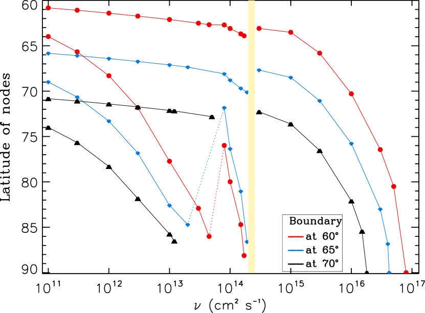
Figure 7: Latitudinal positions of streamfunction nodes as a function of turbulent viscosity, for a meridional flow speed of $10{\rm m}\,{\rm s}^{-1}$ at the boundary, for solar type differential rotation amplitude at the same boundary and three different latitude placements of the boundary. The color code is defined in the figure.

By contrast, when $\nu$ is smaller, the phase of $k_{n}$ is relatively stable and the real and imaginary parts are comparable, leading to a stable pattern of node number and location. In this situation, it is possible to have two or even more nodes. As $\nu$ is increased, all nodes migrate to higher latitudes, because the viscous force is increasingly opposing the Coriolis force. The position of the second node moves more rapidly to higher latitudes with increasing $\nu$ because the amplitude of the polewardmost cell is so much weaker than those at lower latitudes.

Finally, when $\nu$ is greater than in the transition domain, the real part of $k_{n}$ becomes dominant over the imaginary part, largely eliminating the oscillatory component of the solutions. The resulting exponential functions for the streamfunction are much harder to combine into solutions with nodes, so there remain only one or zero nodes. These nodes also migrate toward the poles with increasing $\nu$. In this domain the viscous forces are totally dominant over the Coriolis forces. As $\epsilon\rightarrow 0$ in equation (47), $k_{n}\rightarrow\pm n\pi$, leading to purely exponential functions as solutions for $\Psi_{n}$ in this singular limit. Satisfying the boundary conditions at $x=0,R$ leads to solutions of the form $\Psi_{n}(x)=\Psi_{n}(R)(e^{n\pi x}-e^{-n\pi x})/(e^{n\pi R}-e^{-n\pi R})$. By inspection we see that this solution has no node, consistent with the approach of the curves tracing position of the first node to $90^{\circ}$ on the right hand side of Figure 7. $\epsilon=0$ is equivalent to rotation being zero, so clearly any nodes existent in the solutions must be due to the action of Coriolis forces.

To what degree does the presence and location of the artificial low latitude boundary of the determine the latitude of the first node , especially when it occurs very close to this boundary? We can not know for sure, but we can point out that the influence of Coriolis forces will be very important. If we ignore viscosity, than the latitudinal extent of the meridional flow beyond the boundary should be limited by the so-called ’inertia circle’, which measures the distance over which a meridional flow isw largely turned into the direction of rotation by Coriolis forces. Its amplitude is given at high latitudes approximately by $v/2\Omega$. For a meridional flow speed of $10\,{\rm m}\,{\rm s}^{-1}$, this corresponds to a distance of only about $2\times 10^{3}\,{\rm km}$, extremely short compared to the distance from the boundary to the pole. On the other hand, as we have pointed out earlier, if rotation is absent, there is no mechanism to create nodes at all, and the meridional flow reaches all the way to the pole no matter what the viscosity. Thus in this simple model viscosity is needed to break this constraint and allow the flow to reach closer to the pole.

4.2 Streamfunction typical cases

Here we illustrate how the streamfunction patterns evolve as various parameters are varied. First we show the full range of meridional flow cell structures as a function of turbulent viscosity. Then we illustrate the two quite different ways that the number of streamfunction nodes changes as velocity or turbulent viscosity is changed.

Examples of the full range of possible meridional flow structures found with our model is displayed in Figure 8; the turbulent viscosity increases from top to bottom, over the range $10^{12}-10^{17}{\rm cm}^{2}\,{\rm s}^{-1}$. The examples shown range from having three nodes in the streamfunction (frames a,b) down to zero nodes (frames g,h). This evolution is accomplished first by the countercell expanding to ever higher latitudes, followed by the primary cell doing the same. In all cases, the amplitude of each cell peaks near its low latitude boundary and each cell successively closer to the poles is weaker than its neighbor on the low latitude side. The color contours are logarithmic to allow one to see the weaker cells better; from the right hand column of frames, it is clear that no matter how many nodes there are, on a linear velocity scale, at most only the countercell is detectable, and it is always substantially smaller than the primary cell that is imposed from low latitudes. These results imply that on the Sun, for all viscosity values, it should be possible to detect the countercell, but perhaps none of the smaller cells, if any, occurring poleward of it.

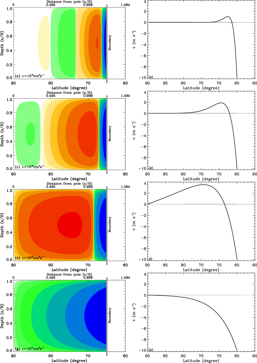
Figure 8: Streamfunction contours and line drawings for $v=10{\rm m}\,{\rm s}^{-1}$ and boundary at $65^{\circ}$ for increasing values of $\nu$. Frames a,b: $10^{12}{\rm cm}^{2}\,{\rm s}^{-1}$; frames c,d: $10^{13}$; frames e,f: $10^{15}$; frame g,h: $10^{17}$ that show wide range of typical streamfunction patterns. Color code same as Figure 8.

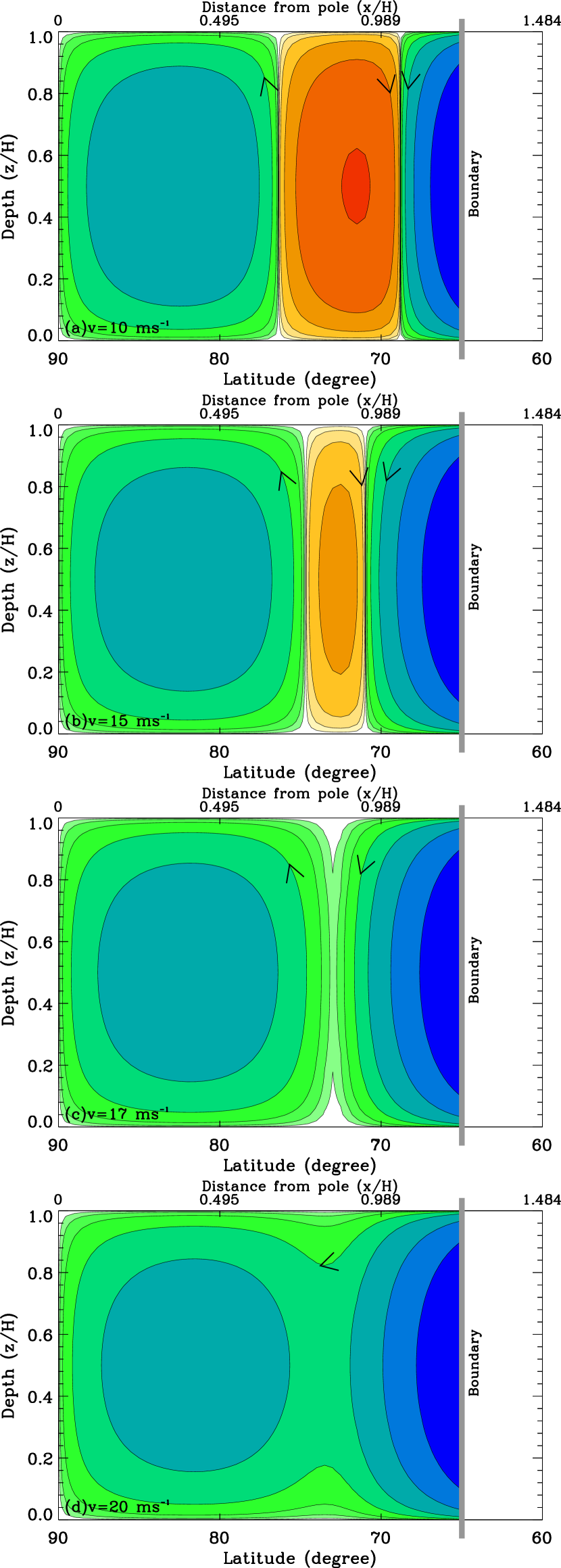
Figure 9: Streamfunction contours (logarithmic; red-yellow areas clockwise flow, green-blue areas counterclockwise flow; arrows indicate the direction of flow) for a sequence of increasing meridional flow speeds at the boundary at $65^{\circ}$, with turbulent viscosity $\nu=10^{14}{\rm cm}^{2}\,{\rm s}^{-1}$, which show the topological changes in the flow patterns as two nodes merge and cancel each other out. In frame a, $v=12{\rm m}\,{\rm s}^{-1}$; frame b, $15{\rm m}\,{\rm s}^{-1}$; frame c, $17{\rm m}\,{\rm s}^{-1}$; frame d, $20{\rm m}\,{\rm s}^{-1}$.

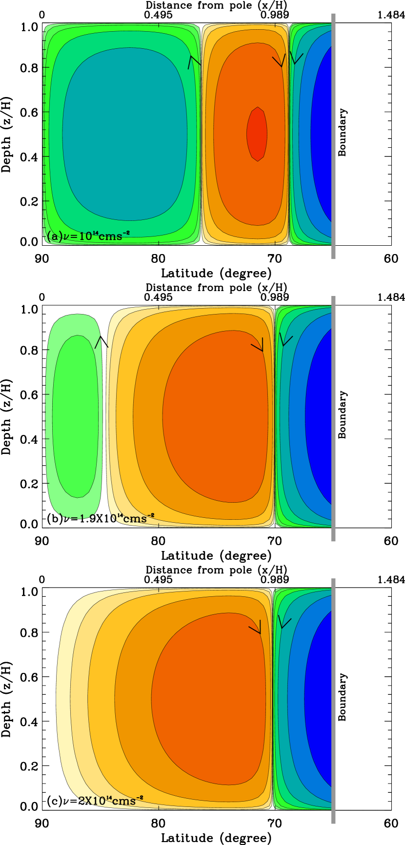
Figure 10: Streamfunction contours for $v=10{\rm m}\,{\rm s}^{-1}$ and boundary at $65^{\circ}$ for increasing values of $\nu=10^{14}{\rm cm}^{2}\,{\rm s}^{-1}$ (frame a); $1.8\times 10^{14}$ (frame b); $2\times 10^{14}$ (frame c) that show evolution of a two node streamfunction pattern into one node as the turbulent viscosity is increased, starting from the same case as in frame a of Figure 9. Color code same as in Figure 8.

Node merger is displayed in Figure 9. In Figure 9 we can see clearly that as the meridional flow speed is increased, node merger, first illustrated in Figures 5, 6 and 7, is accomplished topologically by the two counterclockwise cells increasing their latitudinal dimension toward each other, until the clockwise counter-cell is completely squeezed out and the two counter-clockwise cells in effect merge to create a single cell that reaches all the way to the poles.

By contrast, a very different evolution of the pattern occurs if the boundary flow speed is fixed and the turbulent viscosity is increased. This is shown in Figure 10. Here we see that with increasing $\nu$ by just a factor of two, starting from the same case as shown in Figure 9a, the larger amplitude primary cell and particularly the countercell migrate toward the poles, squeezing the second counterclockwise cell out of existence there. The result is to retain one node, at a relatively low latitude within the polar cap. rather than jumping from two nodes to zero. In this example the turbulent viscosity must be raised two orders of magnitude to eliminate the last node.

We can understand the physics behind this feature if we start with the definition of viscosity. The viscous coefficient is defined by the ratio of shear force per unit area and the gradient of velocity perpendicular to the direction of shear. It is inversely proportional to the velocity gradient. Therefore with the increase in viscous coefficient the velocity gradient should decrease, which means velocities will be more correlated over longer distance. Thus each cell grows bigger in the latitude direction and pushes the next cell, eventually making the polwardmost cell to vanish.

4.3 Differential rotation

In Figure 11 we display solutions for the differential rotation linear velocity that arises from the forcing at the boundary, for the same cases for which streamfunction node positions were plotted in Figure 4. We have not included in these solutions any differential rotation that is independent of $z$ that we might wish to include to allow a closer comparison with solar observations, since, as we have stated earlier, this $z$ independent differential rotation has no effect on the streamfunctions of meridional flow. It is simply a linear function of $x$, declining to zero at the left hand boundary of the cartesian channel from whatever value was specified on the right boundary (black straight line). As stated earlier, it corresponds to constant angular velocity in the cylindrical and spherical shell cases. The total solution for differential rotation would be the sum of the appropriate colored curve and the black line.

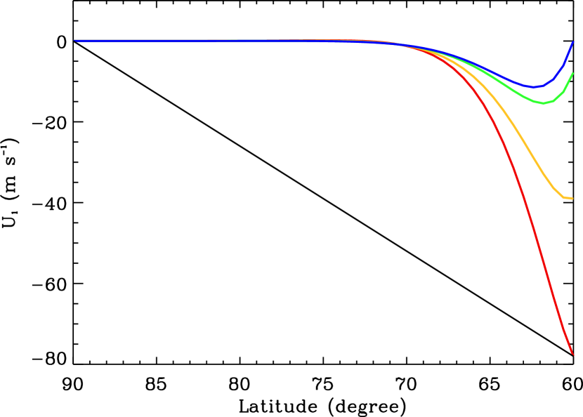
Figure 11: Differential rotation linear velocity that occurs in the interior of the polar cap due to forcing by meridional circulation and differential rotation at the boundary, for the same cases as shown in Figure 4. Color code is the same as in Figure 4. Dimensional linear rotational velocities are calculated relative to a rotating coordinate system whose rotation is that of the solar interior below the convection zone. As a consequence all velocities shown are negative. All linear rotational velocities are zero at the pole (the left boundary of the cartesian analog). The solid black straight line running from $-78\,{\rm m}{\rm s}^{-1}$ at $60^{\circ}$ to zero at $90^{\circ}$ represents approximately the $z$ independent part of the differential rotation linear velocity observed in the Sun at these latitudes. In all cases, the differential rotation at $60^{\circ}$ in the solution matches that of the boundary there. There is no discontinuity in the rotation rate there.

We already saw from Figure 4 that imposing a $z$-dependent differential rotation on the boundary has rather little effect on the positions of nodes in the streamfunction. In Figure 11 we see that the perturbation in differential rotation does not extend that far into the polar cap domain. When no differential rotation is imposed (blue curve) a drop in linear rotation is produced that is confined to the first $10^{\circ}$ of the forcing boundary. This arises due to the Coriolis force from the meridional flow, which itself is declining in amplitude with distance polarward from the forcing boundary. The amplitude of this differential rotation is about that of the observed torsional oscillations.

For much higher forcing by differential rotation at the boundary, this structure is overwhelmed by the simple viscous damping of the rotational flow with poleward distance from the boundary. Coriolis forces from the meridional flow can not maintain these higher values, and the Coriolis force from the imposed differential rotation has only a minor effect on the meridional flow. As a point of comparison, the observed $z$-independent linear differential rotation at high latitudes is given by a straight diagonal line (in black) from the lower right corner of Figure 11, up to the zero point on the left axis, in accordance with the solutions that contain only differential rotation discussed in section 3.6.1. The large difference between this amplitude and that of the four colored curves shown shows how small the differential rotation in our $n=1$ solutions is, except very close to the boundary where the forcing is applied.

5 Discussions and conclusions

We have developed a relatively simple hydrodynamical model of the circulation at high latitudes in the solar convection zone and photosphere that contains only three forces: pressure gradients, viscous and Coriolis forces. The model equations are solved in a cartesian ’analog’ of a spherical polar cap that leaves out curvature effects as well as the large density increase with depth. This system is assumed to be stress-free at the top and bottom, corresponding to the top and bottom of the solar convection zone. It is forced with meridional flow and differential rotation, guided by observations, imposed at the low latitude boundary of the cap, placed at latitudes between $60^{\circ}$ and $70^{\circ}$ latitude. While the inclusion of such a boundary is artificial, it is intended to separate the physics of low and mid-latitudes, responsible for the primary meridional circulation cell that has poleward flow at the top, from the physics active at high latitudes, which should be the primary determinant of the circulation found there.

Our general results are that, as the turbulent viscosity is increased, the number of nodes decreases. As the meridional flow is increased for a given turbulent viscosity, the latitude of a node increases; or, in other words, the node migrates poleward. The first of these results is explained by the viscous forces increasingly overpowering the deflecting effect of the coriolis force to allow the poleward flow of the primary cell to reach a higher latitude. The second is due to the increased poleward momentum of the poleward moving particles that allows them to reach a higher latitude before sinking down to feed the return flow. Overall, we find that our general results are not particularly sensitive to the differential rotation imposed at the boundary, provided it is plausible for the Sun. Unlike for the meridional circulation, changes in the differential rotation of the Sun at all latitudes are very small percentages of the mean differential rotation.

Most interestingly, we find that the decrease in the number of nodes as the turbulent viscosity is increased is not monotonic. In particular, in the neighborhood of $\nu=10^{14}{\rm cm}^{2}\,{\rm s}^{-1}$ in this model, we find that two nodes merge as the meridional flow is increased, leaving no nodes for higher meridional flow at the boundary. This is true even though, for still higher viscosity, there remains one node. Two nodes implies the presence of both a reversed (clockwise) cell and, on its poleward side, a second, weak, counterclockwise cell that has a poleward flow near the top, just as in the primary cell. With the merger of the two nodes, the reverse cell is squeezed out, merging the primary cell with its polar counterpart.

We speculate that it is this phenomenon that could be responsible for the primary cell reaching all the way to the poles during much of cycle 23, whereas there was a node near $65^{\circ}$ in both cycles 22 and the early stages of cycle 24. At present, observations can not tell us whether there is a second node near $80^{\circ}$ as our model predicts. Better observations in the future of velocities at the highest latitudes would obviously be valuable for testing this theory and that of the spherical polar cap that will be developed later. Better information about variations of meridional flow with depth at high latitudes would also be very useful.

Our solutions are for steady flow, but we know that the meridional flow at high latitudes on the Sun changes with time. Given our results, we can expect that a time dependent theory could determine whether changes in meridional flow at the boundary would lead to changes in meridional flow at higher latitudes that agree with observed changes in flow at the highest latitudes. If the Sun merges two nodes with a meridional flow increase, does the model do the same? Does the model predict a merger as a result of an increase in meridional flow that is not observed on the Sun? Questions such as these can only be answered with a time dependent model.

Our results suggest that it may not be necessary to invoke any additional physics to explain changes in the meridional flow cells with time in high latitudes. That does not mean, however, that the presence or importance of such physics can be ruled out at this time.

There are several additional effects that should be included in the high latitude meridional circulation model to make it more realistic. Even keeping the same physics, results from this model using spherical geometry could change significantly. With spherical geometry the meridians converge to the pole, making it harder for as much mass flux to reach the pole as does in the straight channel. In addition, the spherical problem does not separate easily in radius and colatitude due to the Coriolis forces. This has the effect of linking different latitudes and different depths of the flow in ways not present in the cartesian analog. All of these spherical effects should influence the structure of the flow, including the location of nodes in the streamfunction, and how many nodes there are for a given turbulent viscosity.

Within spherical geometry, the flow patterns will change substantially when the density increase with depth through the convection zone is included; the patterns of mass flux, or $\rho v$, could look somewhat like those without the density variation, but the velocity itself should decline substantially with depth. This effect could also change the location and number of nodes present. In this version of the model, effects of the variation of the turbulent viscosity with depth should also be studie; we have already seen that the number and latitude of nodes in the meridional flow is sensitive to the turbulent viscosity used. Allowing this quantity to vary with radius in the spherical case could change the results substantially, as could allowing for the density increase with depth.

In its present form, the model is for axisymmetric motions, and, beyond the turbulent diffusion, our model contains no effect of organized global scale Reynolds stresses. Yet these stresses are surely important in driving the global differential rotation as well as playing a role in the maintenance of the primary meridional cell. We do not know to what latitude these Reynolds stresses reach, but they could be active within the polar cap. Their possible effects on the polar meridional flows should also be considered.

Our model currently also does not include explicitly any thermodynamics. Allowing for departures of the temperature from the adiabatic gradient could be important, particularly at the top and the bottom of the convection zone. Finally, our model is hydrodynamic, so no effects of magnetic fields are included. But the Sun is a dynamo which generates fields, some quite strong, throughout the convection zone, so the effects of these should also be taken into account. One possible effect is that different amplitudes of polar fields might influence the amplitude of meridional flow in high latitudes, as well as the locations of its nodes.

References

- (1)
- Adam & Paldor (2010) Adam, O. & Paldor, N. 2010, GRL, 37, L16801
- Baumann et al (2004) Baumann, I., Schmitt,D., Schüssler, M. & Solanki, S.K. 2004, A & A, 426, 1075
- Beck (2000) Beck, J.G. 2000, Sol.Phys., 191, 47
- Bellon & Sobel (2010) Bellon, G. & Sobel, A.H. 2010, J. Climate, 23, 1760
- Bonanno et al (2005) Bonanno, A., Elstner, D., Belvedere, G. & Rüdiger, G. 2005, AN, 326, 370
- Dikpati & Charbonneau (1999) Dikpati, M. & Charbonneau, P. 1999, ApJ, 518, 508
- Dikpati, de Toma & Gilman (2008) Dikpati, M., de Toma, G. & Gilman, P. A., 2008, ApJ, 675, 920
- Dikpati et al (2010) Dikpati, M., Gilman, P.A., de Toma, G., & Ulrich, R.K., 2010, GRL, 37, L14107
- Friersen, Lu & Chen (2007) Friersen, D.M.W., Lu, J. & Chen, G. 2007, GRL, 34, L18804
- Giles et al (1997) Giles, P.M., Duvall, T.L., Jr., Scherrer, P.H. & Bogart, R.S. 1997, Nature, 390, 52
- Gilman (1979) Gilman, P.A. 1979, ApJ, 231, 284
- Gizon, Birch & Spruit (2010) Gizon, L., Birch, A. & Sprüit, H. 2010, Ann. Rev. Astron. Astrophys., 48, 289
- Gonzalez-Hernandez et al (2008) Gonzalez-Hernandez, I., Kholikov, S., Hill, F., Howe, R. & Komm, R. 2008, Sol. Phys., 252, 235
- Haber et al (2002) Haber, D.A., Hindman, B. W., Toomre, J., Bogart, R. S., Larsen, R. M. & Hill, F. 2002, ApJ, 570, 855
- Heavens et al (2011) Heavens, N.G. et al 2011, JGR, 116, E01010
- Hu, Zhou & Liu (2011) Hu, Y., Zhou, C. & Liu, J. 2011, Adv. Atmos. Sci., 28, 33
- Jiang et al (2008) Jiang, J., Cameron, R., Schmitt, D. & Schüssler, M. 2008, ApJ, 693, 96
- Kaspi, Flierl & Showman (2009) Kaspi, Y., Flierl, G.R. & Showman, A.D. 2009, Icarus, 202, 525
- Kippenhahn (1963) Kippenhahn, R. 1963, ApJ, 137, 664
- Köhler (1970) Köhler, H. 1970, Sol. Phys., 13, 3
- Korty & Schnieder (2008) Korty, R.L. & Schnieder, T. 2008, GRL, 35, L23803
- Küker, Rüdiger & Schültz (2001) Küker, M., Rüdiger, G. & Schültz, M. 2001, A&A, 374, 301
- Küker& Rüdiger (2005) Küker, M., & Rüdiger, G. 2005, A&A, 433, 1023
- Küker& Rüdiger (2008) Küker, M., & Rüdiger, G. 2008, J. Phys:Conf Series 118, 012029
- Komm, Howard & Harvey (1993) Komm, R., Howard, R. F. & Harvey, J. H. 1993, Sol. Phys., 147, 207
- Lebonnois et al (2010) Lebonnois, S. et al 2010, JGR, 115, E06006
- Levine & Schneider (2011) Levine, X.J. & Schneider, T. 2011, J. Atmos. Sci., 68, 769
- Lorenz (1967) Lorenz, E.N. 1967, The Nature and Theory of the General Circulation of the Atmosphere, Geneva (World Meteorological Organization), 161pp
- McIntyre (2007) McIntyre, M.E. 2007, in The Solar Tachocline, ed D.W. Hughes, R. Rosner & N. Weiss (Cambridge: Cambridge Univ. Press), 183
- Miesch et al (2008) Miesch, M. S., Brun, A.S., De Rosa, M. L. & Toomre, J.2008, ApJ, 673, 557
- Rempel (2005) Rempel, M. 2005, ApJ, 622, 1320
- Rüdiger (1989) Rüdiger, G. 1989 ”Differential rotation and stellar convection. Sun and solar-type stars”, Berlin: Akademie Verlag
- Rüdiger & Küker (2002) Rüdiger, G. & Küker, M. 2002, A&A, 385, 308
- Snodgrass & Dailey (1996) Snodgrass, H. B. & Dailey, S.B. 1996, Sol. Phys., 163, 21
- vanda et al (2006) vanda, M., Klvaa, M. & Sobotka, M. 2006, A&A, 458, 301
- vanda et al (2007) vanda, M., Zhao, J. & Kosovichev, A.G. 2007, Sol. Phys., 241, 27
- vanda et al (2008) vanda, M., Klvaa, M., Sobotka, M. & Bumba, V. 2008, A&A, 477, 285
- Thompson (2004) Thompson, M.J. 2004, Astron. Geophys., 45, 4.21
- Ulrich & Boyden (2005) Ulrich, R. K., & Boyden, J. E. 2005, ApJ, 620, L123
- Ulrich (2010) Ulrich, R. K. 2010, ApJ, 725, 658
- Wang & Sheeley (1991) Wang, Y.-M. & Sheeley, N. R. Jr., 1991, ApJ, 375, 761
- Wang, Lean & Sheeley (2005) Wang, Y.-M.,Lean, J. L. & Sheeley, N.R. Jr. 2005, ApJ, 625, 522
- Zhao & Kosovichev (2004) Zhao, J. & Kosovichev, A.G. 2004, ApJ, 203, 776