THE DARK MAGNETISM OF THE UNIVERSE

Abstract

Despite the success of Maxwell’s electromagnetism in the description of the electromagnetic interactions on small scales, we know very little about the behaviour of electromagnetic fields on cosmological distances. Thus, it has been suggested recently that the problems of dark energy and the origin of cosmic magnetic fields could be pointing to a modification of Maxwell’s theory on large scales. Here, we review such a proposal in which the scalar state which is usually eliminated be means of the Lorenz condition is allowed to propagate. On super-Hubble scales, the new mode is essentially given by the temporal component of the electromagnetic potential and contributes as an effective cosmological constant to the energy-momentum tensor. The new state can be generated from quantum fluctuations during inflation and it is shown that the predicted value for the cosmological constant agrees with observations provided inflation took place at the electroweak scale. We also consider more general theories including non-minimal couplings to the space-time curvature in the presence of the temporal electromagnetic background. We show that both in the minimal and non-minimal cases, the modified Maxwell’s equations include new effective current terms which can generate magnetic fields from sub-galactic scales up to the present Hubble horizon. The corresponding amplitudes could be enough to seed a galactic dynamo or even to account for observations just by collapse and differential rotation in the protogalactic cloud.

1 Introduction

Out of the four fundamental interactions, gravity and electromagnetism are the only long-range forces in nature. The standard theories for these two interactions, namely General Relativity (GR) and Maxwell’s electromagnetism have received a vast experimental support in a huge range of scales. GR is able to explain the gravitational phenomena from sub-millimeters distances up to Solar System scales and standard electromagnetism has been probed from the tiny scales involved in high-energy colliders up to distances of order 1.3 A.U. corresponding to the coherence lengths of the magnetic fields dragged by the solar wind[1]. However, despite the enormous success of these two theories, both of them present some unresolved problems when large scales are involved. For GR, cosmological observations require the presence of exotic components in the universe, i.e. dark matter and dark energy. Indeed, some attempts to account for such observations without invoking dark components include infrared modifications of GR. On the other hand, the presence of cosmic magnetic fields found in galaxies, clusters[2, 3, 4] and, very recently[5, 6, 7, 8], also in the voids cannot be accommodated within Maxwell’s theory. This could also be signaling that a more careful analysis of the behavior of electromagnetic fields in cosmological contexts is needed.

A particularly interesting aspect is the quantization of gauge theories in non-trivial spacetimes. The usual quantization procedures of the electromagnetic field in flat spacetime rely on some type of subsidiary condition on the physical states to get rid of the unphysical gauge modes. Although all the approaches are equivalent in flat spacetime, such an equivalence has not been proven in curved background. In fact, the Gupta-Bleuler formalism for the covariant quantization has been shown to present difficulties in a time-dependent spacetime [9, 10]. The BRST method also exhibits similar pathologies in certain spacetimes[11, 12].

Here, we shall review a recent proposal of an extended theory of electromagnetism in which we can avoid the aforementioned difficulties. This extension is based on allowing the propagation of the state that is usually eliminated from the physical Hilbert space by means of the subsidiary condition. We shall show how this theory can be consistently quantized in an expanding universe with three physical states comprising the two polarizations of the usual photons plus one additional scalar state. The remarkable feature of the resulting theory is that the additional state can be generated from quantum fluctuations during inflation and give rise to and effective cosmological constant on large scales, whereas on sub-Hubble scales it leads to the generation of cosmic magnetic fields.

2 Quantization in Minkowski spacetime

The electromagnetic interaction is considered as a paradigm of a well-behaved quantum field theory in Minkowski space-time. Standard Maxwell’s electromagnetism is the theory describing a pure spin one massless particle. Nevertheless, the presence of the local $U(1)$ symmetry in the kinetic term for the photon leads to some difficulties when we want to quantize the theory. The underlying reason for the appearance of these difficulties is the redundancy in the description of the theory due to the $U(1)$ invariance so that we can be wrongly trying to quantize superfluous degrees of freedom corresponding to pure gauge modes. Let us briefly review these difficulties, since it will be useful for our approach.

The starting point will be the Maxwell’s action:

$$S=\int d^{4}x\left(-\frac{1}{4}F_{\mu\nu}F^{\mu\nu}+A_{\mu}J^{\mu}\right)$$ (1)

where $F_{\mu\nu}=\partial_{\mu}A_{\nu}-\partial_{\nu}A_{\mu}$ and $J_{\mu}$ is a conserved current. This action naturally arises when imposing the $U(1)$ gauge symmetry in the sector of charged particles, leading to the symmetry $A_{\mu}\rightarrow A_{\mu}+\partial_{\mu}\chi$ with $\chi$ an arbitrary function of space-time coordinates for the electromagnetic potential. The classical equations of motion derived from this action are the usual Maxwell’s equations:

$$\partial_{\nu}F^{\mu\nu}=J^{\mu}.$$ (2)

The quantization of this theory is not straightforward for a series of reasons that are connected, namely: the vanishing of the conjugate momentum of the temporal component makes not possible to write down its corresponding commutation relation and it is not possible to construct a propagator for the $A_{\mu}$ field. As commented above, the underlying reason for these problems is the presence of the gauge symmetry because that implies the presence of unphysical degrees of freedom which we have to get rid of before proceeding to the quantizations of the physical ones. In order to achieve that, two approaches are commonly used. On one hand, we have the gauge-fixing procedure where we use the gauge symmetry to impose a condition on the electromagnetic potential. Thus for example, we can impose the so-called Lorenz condition $\partial_{\mu}A^{\mu}=0$ so that the equations of motion reduce to:

$$\Box A_{\mu}=J_{\mu}.$$ (3)

Since the Lorenz condition still leaves a residual gauge invariance $A_{\mu}\rightarrow A_{\mu}+\partial_{\mu}\theta$, provided $\Box\theta=0$, we can eliminate one additional component of the $A_{\mu}$ field in the asymptotically free regions (typically $A_{0}$) which means $\vec{\nabla}\cdot\vec{A}=0$. Thus the temporal and longitudinal photons are removed and we are left with the two transverse polarizations of the massless free photon, which are the only modes (with positive energies) which are quantized in this formalism.

On the other hand, in the covariant (Gupta-Bleuler) quantization approach, we start with a modified version of Maxwell’s action, namely:

$$S=\int d^{4}x\left(-\frac{1}{4}F_{\mu\nu}F^{\mu\nu}+\frac{\xi}{2}(\partial_{\mu}A^{\mu})^{2}+A_{\mu}J^{\mu}\right).$$ (4)

that only preserves the residual gauge invariance. The equations of motion obtained from this action now read:

$$\partial_{\nu}F^{\mu\nu} + \xi\partial^{\mu}(\partial_{\nu}A^{\nu})=J^{\mu}.$$ (5)

In order to recover Maxwell’s equations, the Lorenz condition must be imposed so that the $\xi$ term does not contribute. At the classical level this can be achieved by means of appropriate boundary conditions on the field because $\partial_{\nu}A^{\nu}$ evolves as a free scalar field, as obtained from the divergence of (5):

$$\Box(\partial_{\nu}A^{\nu})=0$$ (6)

where we have made use of current conservation. Thus, if $\partial_{\nu}A^{\nu}$ vanishes for large $|t|$, it will vanish at all times. At the quantum level, the Lorenz condition cannot be imposed as an operator identity, but only in the weak sense $\partial_{\nu}A^{\nu\,(+)}|\phi\rangle=0$, where $(+)$ denotes the positive frequency part of the operator and $|\phi\rangle$ stands for a physical state. This condition is equivalent to imposing $[{\bf a}_{0}(\vec{k})+{\bf a}_{\parallel}(\vec{k})]|\phi\rangle=0$, with ${\bf a}_{0}$ and ${\bf a}_{\parallel}$ the annihilation operators corresponding to temporal and longitudinal electromagnetic states. Thus, in the covariant formalism, the physical states contain the same number of temporal and longitudinal photons, so that their energy densities, having opposite signs, cancel each other. Thus, we see that also in this case, the Lorenz condition seems to be essential in order to recover standard Maxwell’s equations and get rid of the negative energy states. Now let us see what happens when moving on to an expanding universe.

3 Quantization in an expanding universe

We shall consider a curved background and, in particular, an expanding universe, and we shall show how consistently imposing the Lorenz condition in the covariant formalism turns out to be difficult to realize [9, 10]. Let us consider the curved space-time version of action (4):

$$S=\int d^{4}x\sqrt{g}\left[-\frac{1}{4}F_{\mu\nu}F^{\mu\nu}+\frac{\xi}{2}(\nabla_{\mu}A^{\mu})^{2}+A_{\mu}J^{\mu}\right]$$ (7)

leading to the corresponding equations of motion:

$$\nabla_{\nu}F^{\mu\nu}+\xi\nabla^{\mu}(\nabla_{\nu}A^{\nu})=J^{\mu}$$ (8)

whose divergence imposes:

$$\Box(\nabla_{\nu}A^{\nu})=0.$$ (9)

We see once again that $\nabla_{\nu}A^{\nu}$ behaves as a free scalar field which is decoupled from the conserved electromagnetic currents, but it is non-conformally coupled to gravity so that it can be excited from quantum vacuum fluctuations by the expanding background in a completely analogous way to the inflaton fluctuations during inflation. Thus, this poses the question of the validity of the Lorenz condition at all times.

In order to illustrate this effect, we will present a toy example. Let us consider quantization in the absence of currents, in a spatially flat expanding background, whose metric is written in conformal time as $ds^{2}=a(\eta)^{2}(d\eta^{2}-d\vec{x}^{2})$ with $a(\eta)=2+\tanh(\eta/\eta_{0})$ where $\eta_{0}$ is constant. This metric has two asymptotically Minkowskian regions in the remote past and far future. We solve the coupled system of equations (8) for the corresponding Fourier modes, which are defined as ${\mathcal{A}}_{\mu}(\eta,\vec{x})=\int d^{3}k{\mathcal{A}}_{\mu\vec{k}}(\eta)e^{i\vec{k}\vec{x}}$. Thus, for a given mode $\vec{k}$, the ${\mathcal{A}}_{\mu}$ field is decomposed into temporal, longitudinal and transverse components. The corresponding equations read:

$${\mathcal{A}}_{0k}^{\prime\prime}-\left[\frac{k^{2}}{\xi}-2{\mathcal{H}}^{\prime}+4{\mathcal{H}}^{2}\right]{\mathcal{A}}_{0k}-2ik\left[\frac{1+\xi}{2\xi}{\mathcal{A}}_{\parallel k}^{\prime}-{\mathcal{H}}{\mathcal{A}}_{\parallel k}\right] = 0$$

$${\mathcal{A}}_{\parallel k}^{\prime\prime}-k^{2}\xi{\mathcal{A}}_{\parallel k}-2ik\xi\left[\frac{1+\xi}{2\xi}{\mathcal{A}}_{0k}^{\prime}+{\mathcal{H}}{\mathcal{A}}_{0k}\right] = 0$$

$$\vec{{\mathcal{A}}}_{\perp k}^{\prime\prime}+k^{2}\vec{{\mathcal{A}}}_{\perp k} = 0$$ (10)

with ${\cal H}=a^{\prime}/a$ and $k=|\vec{k}|$. We see that the transverse modes are decoupled from the background, whereas the temporal and longitudinal ones are non-trivially coupled to each other and to gravity. Let us prepare our system in an initial state $|\phi\rangle$ belonging to the physical Hilbert space, i.e. satisfying $\partial_{\nu}{\mathcal{A}}^{\nu\,(+)}_{in}|\phi\rangle=0$ in the initial flat region. Because of the expansion of the universe, the positive frequency modes in the $in$ region with a given temporal or longitudinal polarization $\lambda$ will become a linear superposition of positive and negative frequency modes in the $out$ region and with different polarizations $\lambda^{\prime}$ (we will work in the Feynman gauge $\xi=-1$). Thus, we have:

$${\mathcal{A}}_{\mu\vec{k}}^{\lambda\;(in)}=\sum_{\lambda^{\prime}=0,\parallel}\left[\alpha_{\lambda\lambda^{\prime}}(\vec{k}){\mathcal{A}}_{\mu\,\vec{k}}^{\lambda^{\prime}\;(out)}+\beta_{\lambda\lambda^{\prime}}(\vec{k})\overline{{\mathcal{A}}_{\mu\,-\vec{k}}^{\lambda^{\prime}\;(out)}}\,\right]$$ (11)

or in terms of creation and annihilation operators:

$${\bf a}_{\lambda}^{(out)}(\vec{k})=\sum_{\lambda^{\prime}=0,\parallel}\left[\alpha_{\lambda\lambda^{\prime}}(\vec{k}){\bf a}_{\lambda^{\prime}}^{(in)}(\vec{k})+\overline{\beta_{\lambda\lambda^{\prime}}(\vec{k})}{\bf a}_{\lambda^{\prime}}^{(in)\dagger}(-\vec{k})\right]$$ (12)

with $\lambda,\lambda^{\prime}=0,\parallel$ and where $\alpha_{\lambda\lambda^{\prime}}$ and $\beta_{\lambda\lambda^{\prime}}$ are the so-called Bogolyubov coefficients (see Ref. Birrell for a detailed discussion), which are normalized in our case according to:

$$\sum_{\rho,\rho^{\prime}=0,\parallel}(\alpha_{\lambda\rho}\,\overline{\alpha_{\lambda^{\prime}\rho^{\prime}}}\,\eta_{\rho\rho^{\prime}}-\beta_{\lambda\rho}\,\overline{\beta_{\lambda^{\prime}\rho^{\prime}}}\,\eta_{\rho\rho^{\prime}})=\eta_{\lambda\lambda^{\prime}}$$ (13)

with $\eta_{\lambda\lambda^{\prime}}=diag(-1,1)$ with $\lambda,\lambda^{\prime}=0,\parallel$. Notice that the normalization is different from the standard one [13], because of the presence of negative norm states.

Thus, the system will end up in a final state which no longer satisfies the weak Lorenz condition i.e. in the out region $\partial_{\nu}{\mathcal{A}}^{\nu\,(+)}_{out}|\phi\rangle\neq 0$. This is shown in Fig. 1, where we have computed the final number of temporal and longitudinal photons $n_{\lambda}^{out}(k)=\sum_{\lambda^{\prime}}|\beta_{\lambda\lambda^{\prime}}(\vec{k})|^{2}$, starting from an initial vacuum state with $n_{0}^{in}(k)=n_{\parallel}^{in}(k)=0$. We see that, as commented above, in the final region $n_{0}^{out}(k)\neq n_{\parallel}^{out}(k)$ and the state no longer satisfies the Lorenz condition. Notice that the failure comes essentially from large scales ($k\eta_{0}\ll 1$), since on small scales ($k\eta_{0}\gg 1$), the Lorenz condition can be restored. This can be easily interpreted from the fact that on small scales the geometry can be considered as essentially Minkowskian.

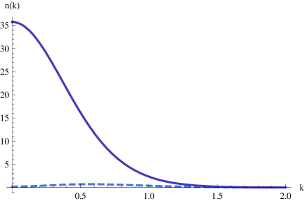
Figure 1: Occupation numbers for temporal (continuous line) and longitudinal (dashed line) photons in the $out$ region vs. $k$ in $\eta_{0}^{-1}$ units.

In order to overcome this problem, it would be possible to use the so called Faddeev-Popov quantization method [14, 15]. In this approach additional unphysical modes (ghosts) are introduced in the theory. They are scalar fields but satisfying fermionic statistics. The physical states of the theory then are chosen as those for which the ghost contribution exactly cancels the contribution from the unphysical gauge modes. However, it has been recently shown that in certain geometries, this type of cancellation can be also problematic [11, 12].

In the following, we shall follow a different approach in order to deal with the difficulties found in the Gupta-Bleuler formalism and we shall explore the possibility of quantizing electromagnetism in an expanding universe without imposing the subsidiary Lorenz condition.

4 Quantization without the Lorenz condition

As we have shown in the previous section, consistently imposing the Lorenz condition is not an easy task. This could actually be signaling a subtle difficulty in formulating a gauge invariant theory of electromagnetism in non-trivial background spacetimes. Here we shall explore the possibility that the fundamental theory of electromagnetism is not given by the gauge invariant action (1), but by the gauge non-invariant action:

$$S=\int d^{4}x\sqrt{g}\left[-\frac{1}{4}F_{\mu\nu}F^{\mu\nu}+\frac{\xi}{2}(\nabla_{\mu}A^{\mu})^{2}+A_{\mu}J^{\mu}\right].$$ (14)

Notice that although this action is not invariant under general gauge transformations, it respects the invariance under residual ones. Moreover, the dynamics of the ordinary transverse photons is not affected, since the extra term only involves temporal and longitudinal polarizations. Let us emphasize that we are assuming that the inclusion of the gauge-breaking term is not a mathematical trick in order to quantize an otherwise gauge-invariant theory, but that such a term is an essential part of a gauge non-invariant electromagnetic theory. Since the fundamental electromagnetic theory is assumed non-invariant under arbitrary gauge transformations, then there is no need to impose the Lorenz constraint in the quantization procedure. Therefore, having removed one constraint, the theory contains one additional degree of freedom. Thus, the general solution for the modified equations (8) can be written as:

$${\mathcal{A}}_{\mu}={\mathcal{A}}_{\mu}^{(1)}+{\mathcal{A}}_{\mu}^{(2)}+{\mathcal{A}}_{\mu}^{(s)}+\partial_{\mu}\theta$$ (15)

where ${\mathcal{A}}_{\mu}^{(i)}$ with $i=1,2$ are the two transverse modes of the massless photon, ${\mathcal{A}}_{\mu}^{(s)}$ is a new scalar state that represents the mode that would have been eliminated if we had imposed the Lorenz condition and, finally, $\partial_{\mu}\theta$ is a purely residual gauge mode, which can be eliminated by means of a residual gauge transformation in the asymptotically free regions, in a completely analogous way to the elimination of the $A_{0}$ component in the Lorenz gauge.

In order to define the quantum theory, apart from the dynamics given by the above Lagrangian, we have to specify the Hilbert space of the physical states. Thus we follow a similar approach to the Lorenz or Coulomb gauge quantization procedure in which the gauge is fixed and then only the physical modes are quantized. In the present case, as commented before, the free theory contains three physical states and we perform the mode expansion of the field with the corresponding creation and annihilation operators:

$${\mathcal{A}}_{\mu}=\int d^{3}\vec{k}\ \sum_{\lambda=1,2,s}\left[{\bf a}_{\lambda}(k){\mathcal{A}}_{\mu k}^{(\lambda)}+{\bf a}_{\lambda}^{\dagger}(k)\overline{{\mathcal{A}}_{\mu k}^{(\lambda})}\,\right]$$ (16)

where the modes are required to be orthonormal with respect to the scalar product[16]

$$\left({\mathcal{A}}^{(\lambda)}_{k},{\mathcal{A}}^{(\lambda^{\prime})}_{k^{\prime}}\right) = i\int_{\Sigma}d\Sigma_{\mu}\left[\,\overline{{\mathcal{A}}_{\nu k}^{(\lambda)}}\;\Pi^{(\lambda^{\prime})\mu\nu}_{k^{\prime}}-\overline{\Pi^{(\lambda)\mu\nu}_{k}}\;{\mathcal{A}}_{\nu k^{\prime}}^{(\lambda^{\prime})}\right]$$ (17)

$$= \delta_{\lambda\lambda^{\prime}}\delta^{(3)}(\vec{k}-\vec{k}^{\prime}),\;\;\;\;\;\lambda,\lambda^{\prime}=1,2,s$$

where $d\Sigma_{\mu}$ is the three-volume element of the Cauchy hypersurfaces. In a Robertson-Walker metric in conformal time, it reads $d\Sigma_{\mu}=a^{4}(\eta)(d^{3}x,0,0,0)$. The generalized conjugate momenta are defined as:

$$\Pi^{\mu\nu}=-(F^{\mu\nu}-\xi g^{\mu\nu}\nabla_{\rho}A^{\rho})$$ (18)

Notice that the three modes can be chosen to have positive normalization. The equal-time commutation relations:

$$\left[{\mathcal{A}}_{\mu}(\eta,\vec{x}),{\mathcal{A}}_{\nu}(\eta,\vec{x}\,^{\prime})\right]=\left[\Pi^{0\mu}(\eta,\vec{x}),\Pi^{0\nu}(\eta,\vec{x}^{\prime})\right]=0$$ (19)

and

$$\left[{\mathcal{A}}_{\mu}(\eta,\vec{x}),\Pi^{0\nu}(\eta,\vec{x}\,^{\prime})\right]=i\frac{\delta_{\mu}^{\;\nu}}{\sqrt{g}}\delta^{(3)}(\vec{x}-\vec{x}\,^{\prime})$$ (20)

can be seen to imply the canonical commutation relations

$$\left[{\bf a}_{\lambda}(\vec{k}),{\bf a}_{\lambda^{\prime}}^{\dagger}(\vec{k^{\prime}})\right]=\delta_{\lambda\lambda^{\prime}}\delta^{(3)}(\vec{k}-\vec{k^{\prime}}),\;\;\;\lambda,\lambda^{\prime}=1,2,s$$ (21)

by means of the normalization condition in (17). Notice that the sign of the commutators is positive for the three physical states, i.e. there are no negative norm states in the theory, which in turn guarantees that there are no negative energy states as we will see below in an explicit example.

Notice that unlike the quantization in the Gupta-Bleuler formalism, in this extended theory it is not possible to eliminate the unphysical degree of freedom in a manifestly covariant way.

Since $\nabla_{\mu}{\mathcal{A}}^{\mu}$ evolves as a minimally coupled scalar field, as shown in (9), on sub-Hubble scales ($|k\eta|\gg 1$), we find that for arbitrary background evolution, $|\nabla_{\mu}{\mathcal{A}}^{(s)\mu}_{k}|\propto e^{\pm ik\eta}a^{-1}$, i.e. the mode behaves as a plane-wave with decaying amplitude giving rise through (8) to a longitudinal electric wave. This is an important difference with respect to ordinary electromagnetism, since the modified theory allows the propagation of longitudinal electric waves in the absence of sources. As we will show below, these longitudinal fields in the presence of a highly conductive plasma could induce the production of large scale magnetic fields.

On the other hand, on super-Hubble scales ($|k\eta|\ll 1$), $|\nabla_{\mu}{\mathcal{A}}^{(s)\mu}_{k}|=const.$ which implies that the field contributes as a cosmological constant in (7). Indeed, the energy-momentum tensor derived from (7) reads:

$$T_{\mu\nu} = -F_{\mu\alpha}F_{\nu}^{\;\;\alpha}+\frac{1}{4}g_{\mu\nu}F_{\alpha\beta}F^{\alpha\beta}$$ (22)

$$+ \frac{\xi}{2}\left[g_{\mu\nu}\left[\left(\nabla_{\alpha}A^{\alpha}\right)^{2}+2A^{\alpha}\nabla_{\alpha}\left(\nabla_{\beta}A^{\beta}\right)\right]-4A_{(\mu}\nabla_{\nu)}\left(\nabla_{\alpha}A^{\alpha}\right)\right]$$

Notice that for the scalar electromagnetic mode in the super-Hubble limit, the contributions involving $F_{\mu\nu}$ vanish and only the piece proportional to $\xi$ is relevant. Thus, it can be easily seen that, since in this case $\nabla_{\alpha}A^{\alpha}=constant$, the energy-momentum tensor is just given by:

$$T_{\mu\nu}=\frac{\xi}{2}g_{\mu\nu}(\nabla_{\alpha}A^{\alpha})^{2}$$ (23)

which is the energy-momentum tensor of a cosmological constant and whose value is given by the four-divergence of the electromagnetic field. In fact, this result is not specific of FLRW spacetimes, but it is valid for any geometry. In a field configuration with the vector potential given by the gradient of a scalar that is not a pure residual gauge mode, i.e., $A_{\mu}=\partial_{\mu}\phi$ with $\Box\phi\neq 0$, we obtain that $F_{\mu\nu}$ vanishes. Thus, from the equations of motion (8) in the absence of external currents we get that $\nabla_{\mu}A^{\mu}$ is constant so that the energy momentum tensor reduces once again to the form (23). This implies that we can always reproduce the solutions of Einstein equations plus a cosmological constant with $\nabla_{\mu}A^{\mu}$ playing the role of the effective cosmological constant.

5 Quantum fluctuations during inflation

Let us consider an explicit example which is given by the quantization in an inflationary de Sitter spacetime with $a(\eta)=-1/(H_{I}\eta)$, with $H_{I}$ the constant Hubble parameter during inflation. The explicit solution in the case $\xi=1/3$ for the normalized scalar state is:

$${\mathcal{A}}_{0k}^{(s)}= \frac{-1}{(2\pi)^{3/2}}\frac{i}{\sqrt{2k}}\left\{k\eta e^{-ik\eta}+\frac{1}{k\eta}\left[\frac{1}{2}(1+ik\eta)e^{-ik\eta}-k^{2}\eta^{2}e^{ik\eta}E_{1}(2ik\eta)\right]\right\}e^{i\vec{k}\vec{x}}$$

$${\mathcal{A}}_{\parallel k}^{(s)}= \frac{1}{(2\pi)^{3/2}}\frac{1}{\sqrt{2k}}\left\{(1+ik\eta)e^{-ik\eta}-\left[\frac{3}{2}e^{-ik\eta}+(1-ik\eta)e^{ik\eta}E_{1}(2ik\eta)\right]\right\}e^{i\vec{k}\vec{x}}$$

where $E_{1}(x)=\int_{1}^{\infty}e^{-tx}/tdt$ is the exponential integral function. Using this solution, we find:

$$\nabla_{\mu}{\mathcal{A}}^{(s)\mu}_{k}=-\frac{a^{-2}(\eta)}{(2\pi)^{3/2}}\frac{ik}{\sqrt{2k}}\frac{3}{2}\frac{(1+ik\eta)}{k^{2}\eta^{2}}e^{-ik\eta+i\vec{k}\vec{x}}$$ (25)

so that the field is suppressed in the sub-Hubble limit as $\nabla_{\mu}{\mathcal{A}}^{(s)\mu}_{k}\sim{\cal O}((k\eta)^{-2})$.

On the other hand, from the energy density given by $\rho_{A}=T^{0}_{\;\;0}$, we obtain in the sub-Hubble limit the corresponding Hamiltonian, which is given by:

$$H=\frac{1}{2}\int\frac{d^{3}\vec{k}}{a^{4}(\eta)}k\sum_{\lambda=1,2,s}\left[{\bf a}_{\lambda}^{\dagger}(\vec{k}){\bf a}_{\lambda}(\vec{k})+{\bf a}_{\lambda}(\vec{k}){\bf a}_{\lambda}^{\dagger}(\vec{k})\right].$$ (26)

We see that the theory does not contain negative energy states (ghosts).

Also, from (LABEL:scalar) it is possible to obtain the dispersion of the effective cosmological constant during inflation:

$$\langle 0|(\nabla_{\mu}{\mathcal{A}}^{\mu})^{2}|0\rangle=\int\frac{dk}{k}P_{A}(k)$$ (27)

with $P_{A}(k)=4\pi k^{3}|\nabla_{\mu}{\mathcal{A}}^{(s)\mu}_{k}|^{2}$. In the super-Hubble limit, we get in a quasi-de Sitter inflationary phase characterized by a slow-roll parameter $\epsilon$:

$$P_{\nabla A}(k)=\frac{9H_{k_{0}}^{4}}{16\pi^{2}}\left(\frac{k}{k_{0}}\right)^{-4\epsilon}$$ (28)

where $H_{k_{0}}$ is the Hubble parameter when the $k_{0}$ mode left the horizon [17, 18]. Notice that this result implies that $\rho_{A}\sim(H_{k_{0}})^{4}$. The measured value of the cosmological constant then requires $H_{k_{0}}\sim 10^{-3}$ eV, which corresponds to an inflationary scale $M_{I}\sim 1$ TeV. Thus we see that the cosmological constant scale can be naturally explained in terms of physics at the electroweak scale. This is one of the most relevant aspects of the present model in which, unlike existing dark energy theories based on scalar fields, dark energy can be generated without including any potential term or dimensional constant. It is also interesting to note that the required scale is the electroweak scale, since for higher energies electromagnetism becomes unified with the electroweak interactions so that it would not make sense to speak about photons anymore.

On the other hand, despite the fact that the background evolution in the present case is the same as in $\Lambda$CDM, the evolution of metric perturbations could be different. We have calculated the evolution of metric, matter density and electromagnetic perturbations [19]. The propagation speeds of scalar, vector and tensor perturbations are found to be real and equal to the speed of light, so that the theory is classically stable. On the other hand, it is possible to see that all the parametrized post-Newtonian (PPN) parameters [20] agree with those of General Relativity, i.e. the theory is compatible with all the local gravity constraints for any value of the homogeneous background electromagnetic field [17, 18, 21].

Concerning the evolution of scalar perturbations, we find that the only relevant deviations with respect to $\Lambda$CDM appear on large scales $k\sim H_{0}$ and that they depend on the primordial spectrum of electromagnetic fluctuations. However, the effects on the CMB temperature and matter power spectra are compatible with observations except for very large primordial fluctuations [19].

6 Generation of cosmic magnetic fields

By looking at the equations of motion, we realize that the $\xi$-term can be interpreted as a conserved effective current: $-\xi\nabla^{\mu}(\nabla_{\nu}A^{\nu})\equiv J_{\nabla\cdot A}^{\mu}$ which, according to (9), satisfies the conservation equation $\nabla_{\mu}J_{\nabla\cdot A}^{\mu}=0$. More precisely, the equations of motion can be recast in the form:

$$\nabla_{\nu}F^{\mu\nu}=J^{\mu}_{T}$$ (29)

with $J^{\mu}_{T}=J^{\mu}+J^{\mu}_{\nabla\cdot A}$ and $\nabla_{\mu}J^{\mu}_{T}=0$. Physically, this means that, while the new scalar mode can only be excited gravitationally, once it is produced it will generally give rise to an effective source of electromagnetic fields. Therefore, the modified theory is described by ordinary Maxwell’s equations with an additional ”external” current. For an observer with four-velocity $u^{\mu}$ moving with the cosmic plasma, it is possible to decompose the Faraday tensor in its electric and magnetic parts as: $F_{\mu\nu}=2E_{[\mu}u_{\nu]}+\frac{\epsilon_{\mu\nu\rho\sigma}}{\sqrt{g}}B^{\rho}u^{\sigma}$, where $E^{\mu}=F^{\mu\nu}u_{\nu}$ and $B^{\mu}=\epsilon^{\mu\nu\rho\sigma}/(2\sqrt{g})F_{\rho\sigma}u_{\nu}$. Due to the infinite conductivity of the plasma, Ohm’s law $J^{\mu}-u^{\mu}u_{\nu}J^{\nu}=\sigma F^{\mu\nu}u_{\nu}$ implies $E^{\mu}=0$. Therefore, in that case the only contribution would come from the magnetic part. Thus, from Maxwell’s equations, we can get:

$$F^{\mu\nu}_{\;\;\;\;;\nu}u_{\mu}=\frac{\epsilon^{\mu\nu\rho\sigma}}{\sqrt{g}}B_{\rho}u_{\sigma\,;\nu}u_{\mu}=J^{\mu}_{\nabla\cdot A}u_{\mu}$$ (30)

where we have made use of the electric neutrality of the cosmic plasma, i.e. $J_{\mu}u^{\mu}=0$. For comoving observers in a FLRW metric we can write (see also Ref. FC):

$$\vec{\omega}\cdot\vec{B}=\rho_{g}^{0}$$ (31)

where $\vec{v}=d\vec{x}/d\eta$ is the conformal time fluid velocity, $\vec{\omega}=\vec{\nabla}\times\vec{v}$ is the fluid vorticity, $\rho_{g}^{0}$ is the effective charge density today and the $\vec{B}$ components scale as $B_{i}\propto 1/a$ as can be easily obtained from $\nabla_{\mu}\tilde{F}^{\mu\nu}=0$, with $\tilde{F}$ the dual of the Faraday tensor, to the lowest order in $v$. Therefore, because of the presence of the effective charge density generated by the scalar state, we shall have both magnetic field and vorticity. Moreover, from the cosmological evolution of the magnetic field and the electric charge density given above, we obtain that $|\vec{\omega}|\propto a$, from radiation era until present.

We should remind here that $\nabla_{\nu}A^{\nu}$ is constant on super-Hubble scales and starts decaying as $1/a$ once the mode reenters the Hubble radius. Thus, today, a mode $k$ will have been suppressed by a factor $a_{in}(k)$ (we are assuming that the scale factor today is $a_{0}=1$). This factor will be given by: $a_{in}(k)=\Omega_{M}H_{0}^{2}/k^{2}$ for modes entering the Hubble radius in the matter era, i.e. for $k<k_{eq}$ with $k_{eq}\simeq(14\,\mbox{Mpc})^{-1}\Omega_{M}h^{2}$ the value of the mode which entered at matter-radiation equality. For $k>k_{eq}$ we have $a_{in}(k)=\sqrt{2\Omega_{M}}(1+z_{eq})^{-1/2}H_{0}/k$. It is then possible to compute from (28) the corresponding power spectrum for the effective electric charge density today $\rho_{g}^{0}=J_{\nabla\cdot A}^{0}=-\xi\partial_{0}(\nabla_{\nu}A^{\nu})$. Thus from:

$$\langle\rho(\vec{k})\rho^{*}(\vec{h})\rangle=(2\pi)^{3}\delta(\vec{k}-\vec{h})\rho^{2}(k)$$ (32)

we define $P_{\rho}(k)=\frac{k^{3}}{2\pi^{2}}\rho^{2}(k)$, which is given by:

$$P_{\rho}(k)=\left\{\begin{array}[]{cc}0,&k<H_{0}\\ &\\ \frac{\Omega_{M}^{2}H_{0}^{2}H_{k0}^{4}}{16\pi^{2}}\left(\frac{k}{k_{0}}\right)^{-4\epsilon-2},&H_{0}<k<k_{eq}\\ &\\ \frac{2\Omega_{M}H_{0}^{2}H_{k0}^{4}}{16\pi^{2}(1+z_{eq})}\left(\frac{k}{k_{0}}\right)^{-4\epsilon},&k>k_{eq}.\end{array}\right.$$ (38)

Therefore the corresponding charge variance will read: $\langle\rho^{2}\rangle=\int\frac{dk}{k}P_{\rho}(k)$. For modes entering the Hubble radius in the radiation era, the power spectrum is nearly scale invariant. Also, due to the constancy of $\nabla_{\nu}A^{\nu}$ on super-Hubble scales, the effective charge density power spectrum is negligible on such scales, so that we do not expect magnetic field nor vorticity generation on those scales. Notice that, on sub-Hubble scales, the effective charge density generates longitudinal electric fields whose present amplitude would be precisely $E_{L}\simeq\nabla_{\nu}A^{\nu}$. This implies that a generic prediction of the extended theory would be the existence of a cosmic background of longitudinal electric waves, whose power spectrum is given by (28).

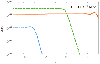
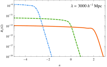
Figure 2: Lower limits on the magnetic fields generated on galactic scales (left panel) and Hubble horizon scales (right panel) in terms of the magnetic spectral index $n$ for different values of the vorticity spectral index $m$. Dot-dashed blue for $m=0$, dashed green for $m\simeq-3$ and full red for $m\simeq-5$.

Using (31), it is possible to translate the existing upper limits on vorticity coming from CMB anisotropies [22] into lower limits on the amplitude of the magnetic fields generated by this mechanism. This indeed represents a discriminating signature of this model because the presence of such magnetics fields is a clear prediction of the theory. We will consider for simplicity magnetic field and vorticity as gaussian stochastic variables such that:

$$\langle B_{i}(\vec{k})B_{j}^{*}(\vec{h})\rangle = \frac{(2\pi)^{3}}{2}P_{ij}\delta(\vec{k}-\vec{h})B^{2}(k)$$

$$\langle\omega_{i}(\vec{k})\omega_{j}^{*}(\vec{h})\rangle = \frac{(2\pi)^{3}}{2}P_{ij}\delta(\vec{k}-\vec{h})\omega^{2}(k)$$ (39)

with $B^{2}(k)=Bk^{n}$, $\omega^{2}(k)=\Omega k^{m}$ and where $P_{ij}=\delta_{ij}-\hat{k}_{i}\hat{k}_{j}$ is introduced because of the transversality properties of $B_{i}$ and $\omega_{i}$. The spectral indices $n$ and $m$ are in principle arbitrary. In Fig. 2 we show the lower limits on the magnetic fields generated by this mechanism on scales $\lambda=0.1h^{-1}$ Mpc, and $\lambda=3000h^{-1}$ Mpc, also for inflation at the electroweak scale. We see that fields can be generated with sufficiently large amplitudes in order to seed a galactic dynamo or even to account for observations just by collapse and differential rotation of the protogalactic cloud [23]. Moreover, they could be also compatible with recent extra-galactic observations[5, 6].

7 Non-minimal couplings

We shall end by generalizing the previous results to include non-minimal couplings to curvature:

$$S=\int d^{4}x\sqrt{-g}\left[-\frac{1}{4}F_{\mu\nu}F^{\mu\nu}+\frac{\xi}{2}(\nabla_{\mu}A^{\mu})^{2}+\sigma G_{\mu\nu}A^{\mu}A^{\nu}\right].$$ (40)

Notice that we are not introducing any new dimensional parameter, being $\sigma$ a dimensionless constant. The particular non-minimal coupling has been chosen so that the induced effective electromagnetic current $J_{g}^{\mu}=2\sigma G^{\mu\nu}A_{\nu}$ is covariantly conserved in the weak field limit, which is achieved thanks to the divergenceless of the Einstein tensor $G_{\mu\nu}$. The most stringent constraint on $\sigma$ comes from PPN measurements and it is given by $|\sigma|\mathrel{\mathop{\kern 0.0pt\hbox to0.0pt{\raise 0.86108pt\hbox{$<$}\hss}}\lower 3.87495pt\hbox{\kern-1.90002pt$\sim$}}10^{-5}$. Moreover, the smallness of $\sigma$ guarantees the stability of the theory and that the cosmological evolution of the homogeneous mode becomes modified in a negligible way by the presence of the non-minimal coupling. This ensures that the inflationary generation and cosmological evolution discussed in previous sections for the minimal theory is also a good description in the non-minimal case (see Ref. nonminimal for a more detail discussion).

In the following we shall show how the non-minmal coupling gives rise to non-trivial electromagnetic effects generated by massive bodies even if they are electrically neutral. To that end, we shall assume a small perturbation around Minkowski with a constant background vector field of the form $A_{\mu}=\bar{A}_{0}\delta^{0}_{\mu}$. Thus, the effective current becomes $J_{g}^{\mu}=2\sigma G^{\mu 0}\bar{A}_{0}$ and, using Einstein equations to relate $G^{\mu\nu}$ to the matter content, we obtain:

$$J_{g}^{\mu}=16\pi G\sigma T^{\mu 0}\bar{A}_{0}$$ (41)

so that the effective electromagnetic current is essentially determined by the four-momentum density. Moreover, if we assume $T^{\mu\nu}=(\rho+p)u^{\mu}u^{\nu}-p\eta^{\mu\nu}$ at first order, we can see that the energy density of any perfect fluid has an associated electric charge density given, for small velocities, by:

$$\rho_{g}=J_{g}^{0}=16\pi G\sigma\rho\bar{A}_{0}$$ (42)

and the three-momentum density generates an electric current density given by

$$\vec{J}_{g}=16\pi G\sigma(\rho+p)\vec{v}\bar{A}_{0}$$ (43)

Thus, this theory effectively realizes the old conjecture by Schuster, Einstein and Blackett [25, 26, 27] of gravitational magnetism, i.e. neutral mass currents can generate electromagnetic fields.

In the case of a particle of mass $m$ at rest, (42) introduces a small contribution to the active electric charge (the source of the electromagnetic field), given by $\Delta q=16\pi G\sigma m\bar{A}_{0}\simeq 15\sigma(m/M_{P})$, but leaving unmodified its passive electric charge (that determining the coupling to the electromagnetic field). This effect implies a difference in the active charge of electrons and protons because of their mass difference and, furthermore, provides neutrons with a non-vanishing active electric charge. However, the effect is very small in both cases $\Delta q\simeq 4\sigma 10^{-18}e$ where $e=0.303$ is the electron charge in Heaviside-Lorentz units. Present limits on the electron-proton charge asymmetry and neutron charge are both of the order $10^{-21}e$ [28], implying $|\sigma|\mathrel{\mathop{\kern 0.0pt\hbox to0.0pt{\raise 0.86108pt\hbox{$<$}\hss}}\lower 3.87495pt\hbox{\kern-1.90002pt$\sim$}}10^{-3}$ which is less stringent than the PPN limit discussed before.

On the other hand, for any compact object, the effective electric current will generate an intrinsic magnetic moment given by:

$$\vec{m}=\beta\frac{\sqrt{G}}{2}\vec{L}$$ (44)

with $\vec{L}$ the corresponding angular momentum and $\beta=16\pi\sqrt{G}\sigma\bar{A}_{0}$ a constant parameter. This relation resembles the Schuster-Blackett law, which is a purely empirical relation between the magnetic moment and the angular momenta found in a wide range of astrophysical objects from planets, to galaxies, including those related to the presence of rotating neutron stars such as GRB or magnetars [29, 30]. In any case, the observational evidence on this relation is still not conclusive. From observations, the $\beta$ parameter ranges from 0.001 to 0.1. Imposing the PPN limits on the $\sigma$ parameter, we find $\beta\mathrel{\mathop{\kern 0.0pt\hbox to0.0pt{\raise 0.86108pt\hbox{$<$}\hss}}\lower 3.87495pt\hbox{\kern-1.90002pt$\sim$}}10^{-4}$, which is just below the observed range. Thus for a typical spiral galaxy, a direct calculation provides: $B\sim\sigma 10^{-4}$ G, i.e. according to the PPN limits, the field strength could reach $10^{-9}$ G without amplification.

8 Discussion

We have reviewed the extended electromagnetic theory in which a gauge-fixing term is promoted into a physical contribution in the fundamental action. The quantization of the free theory can be performed without having to impose any subsidiary condition at the price of introducing an additional degree of freedom. This new mode can be gravitationally produced from quantum fluctuations during inflation and its amplitude will be determined precisely by the scale at which inflation takes place. In the subsequent cosmological evolution, this new mode has two effects. On super-Hubble scales, it behaves as an effective cosmological constant whose observed value can be explained if inflation occurred at the electroweak scale. On sub-Hubble scales, the additional mode gives rise to a stochastic background of longitudinal electric waves that generate magnetic fields from sub-galactic scales up to the present Hubble radius. On the other hand, we have also considered the effects of non-minimal couplings in the presence of the temporal electromagnetic mode and shown that in such a case, neutral massive objects can act as sources of electromagnetic fields thus implementing the old conjecture by Schuster, Einstein and Blackett of gravitational magnetism.

The theory studied in this work shows how a modification of electromagnetism which does not require the introduction of new fields, dimensional parameters or potential terms could provide a simple explanation for the tiny value of the cosmological constant and, at the same time, a mechanism for the generation of magnetic fields on cosmological scales. Some open questions still remain to be studied such as the inclusion of electromagnetic interactions in the theory, since all the analysis performed so far are limited to the free theory. Also, it would be interesting to know the behaviour of the new mode in more general background space-times in order to determine the viability of the model from the theoretical and phenomenological point of views. Finally, the possibility of detecting the longitudinal electric wave background generated during inflation could provide a clear signal of the modification of electromagnetism on cosmological scales.

Acknowledgments: This work has been supported by MICINN (Spain) project numbers FIS 2008-01323 and FPA 2008-00592, CAM/UCM 910309 and MICINN Consolider-Ingenio MULTIDARK CSD2009-00064. JBJ is also supported by the Ministerio de Educación under the postdoctoral contract EX2009-0305.

References

- [1] A. S. Goldhaber, M. M. Nieto, Rev. Mod. Phys. 82 (2010) 939-979.
- [2] L. M. Widrow, Rev. Mod. Phys. 74 (2002) 775.
- [3] R. M. Kulsrud and E. G. Zweibel, Rept. Prog. Phys. 71 (2008) 0046091;.
- [4] P. P. Kronberg, Rept. Prog. Phys. 57 (1994) 325.
- [5] A. Neronov and I. Vovk, Science 328 (2010) 73;
- [6] F. Tavecchio, et al., MNRAS, 406: L70-L74,2010.
- [7] S. i. Ando, A. Kusenko, Astrophys. J. 722 (2010) L39.
- [8] A. Neronov, D. V. Semikoz, P. G. Tinyakov et al., [arXiv:1006.0164 [astro-ph.HE]].
- [9] A. Higuchi, L. Parker and Y. Wang, Phys. Rev. D 42, 4078 (1990).
- [10] J. Beltrán Jiménez and A.L. Maroto, Phys. Lett. B 686 (2010) 175.
- [11] A. R. Zhitnitsky, Phys. Rev. D 82 (2010) 103520.
- [12] N. Ohta, Phys. Lett. B695: 41-44 (2011).
- [13] Birrell, N.D. and Davies, P.C.W., Quantum fields in curved space, Cambridge University Press, 1982, ISBN: 0-521-27858-9.
- [14] S. L. Adler, J. Lieberman, and Y. J. Ng, Ann. Phys. 106 (1977) 279.
- [15] M. R. Brown and A. C. Ottewill,, Phys. Rev. D34 (1986) 1776–1786.
- [16] M. J. Pfenning, Phys. Rev. D65 (2002) 024009.
- [17] J. Beltrán Jiménez and A.L. Maroto, JCAP 0903 (2009) 016.
- [18] J. Beltrán Jiménez and A.L. Maroto, Int. J. Mod. Phys. D 18 (2009) 2243.
- [19] J. B. Jimenez, T. S. Koivisto, A. L. Maroto and D. F. Mota, JCAP 0910 (2009) 029.
- [20] C. Will, Theory and experiment in gravitational physics, Cambridge University Press, (1993).
- [21] J. B. Jimenez and A. L. Maroto, JCAP 0902 (2009) 025.
- [22] C. Caprini and P. G. Ferreira, JCAP 0502 (2005) 006.
- [23] J. Beltrán Jiménez, A. L. Maroto, Phys. Rev. D83: 023514 (2011).
- [24] J. Beltrán Jiménez, A. L. Maroto, JCAP 1012: 025 (2010).
- [25] A. Schuster, Proc. Lond. Phys. Soc. 24 (1912) 121.
- [26] A. Einstein, Schw. Naturf. Ges. Verh. 105 Pt. 2, 85 (1924) S. Saunders S and H.R. Brown, Philosophy of Vacuum (Oxford: Clarendon) (1991).
- [27] P. M. S. Blackett, Nature 159 (1947) 658.
- [28] C. Amsler et al. (Particle Data Group), Phys. Lett. B 667 (2008) 1.
- [29] R. Opher and U. F. Wichoski, Phys. Rev. Lett. 78 (1997) 787.
- [30] R. da Silva de Souza, R. Opher, JCAP 1002 (2010) 022.