Extending spin ice concepts to another geometry: the artificial triangular spin ice

Abstract

In this work we propose and study a realization of an artificial spin ice-like system in a triangular geometry, which unlike square and kagome artificial spin ice, is not based on any real material. At each vertex of the lattice, the “ice-like rule” dictates that three spins must point inward while the other three must point outward. We have studied the system’s ground-state and the lowest energy excitations as well as the thermodynamic properties of the system. Our results show that, despite fundamental differences in the vertices topologies as compared to the artificial square spin ice, in the triangular array the lowest energy excitations also behave as a kind of Nambu monopoles (two opposite monopoles connected by an energetic string). Indeed, our results suggest that the monopoles charge intensity may have a universal value while the string tension could be tuned by changing the system’s geometry, probably allowing the design of systems with different string tensions. Our Monte Carlo findings suggest a phase transition in the Ising universality class where the mean distance between monopoles and anti-monopoles increases considerably at the critical temperature. The differences on the vertices topologies seem to facilitate the experimental achievement of the system’s ground-state, thereby allowing a more detailed experimental study of the system’s properties.

I Introduction

Geometrical frustration and fractionalization are key concepts in modern condensed matter theory. While the former is related to the impossibility of simultaneously minimize the energy for all constituents of a system due to geometrical constraints, the latter is related to the appearance of collective excitations that carry only a fraction of the elementary constituents properties. In some systems these phenomena are closely related, as is the case of spin ice materials (Dy₂Ti₂O₇ and Ho₂Ti₂O₇) Castelnovo08 ; Fennell09 ; Morris09 ; Bramwell09 ; Kadowaki09 ; Jaubert09 ; Giblin11 . There, due to a geometrical frustration, the energy is minimized by the appearance of the two-in/two-out ice rule, where at each vertex of a lattice two spins point inward and two outward. Violations of this rule are viewed thus as a fraction of a dipole Castelnovo08 , since these collective excitations behave as magnetic monopoles, constituting the first example of fractionalization in three-dimensional ($3d$) materials.

With the aid of modern experimental techniques, mainly the capability to construct and manipulate nanostructured systems, artificial arrays with properties very similar to the spin ice material were recently built Wang06 ; Li10 ; Zabel09 ; Ladak10 ; Mengotti10 . In particular, in an artificial frustrated two-dimensional ($2d$) square array that mimic the spin ice behavior, the excitations above the ground-state are viewed as a kind of Nambu magnetic monopoles Nambu77 ; Mol09 ; Mol10 ; Morgan10 ; Moller09 , since the end points of the energetic string behave like particles with magnetic charge, which leads to a Coulomb interaction (we remark that the Coulomb is a particular case of the Yukawa potential present in the Nambu calculations). Therefore, there is, of course, a huge interest in accessing the ground-state of the artificial square spin ice (ASSI) to test theoretical predictions concerning the appearance and behavior of monopoles excitations Moller06 ; Silva12 ; Budrikis10 ; Kapaklis11 . However demagnetization protocols Ke08 ; Nisoli07 ; Nisoli10 used so far were not able to drive the ASSI to its lowest energy state. Morgan et al Morgan10 successfully achieved what seems to be the thermalization of the ASSI during fabrication, although, they could not obtain a single ground-state domain.

In this work we investigate if the same fractionalization phenomenon manifested in the ASSI is also present in another artificial setting. We consider here a particular realization of an artificial spin ice in a triangular geometry. Unlike the square and kagome spin ice, our proposal is not based in any real material and were motivated by inquiring what changes arise when the geometry of an artificially frustrated magnetic system is not the usual for typical spin ices. By doing this we have found that in the triangular geometry the ground-state is much likely to be easily obtained experimentally, allowing the experimental investigation of the existence and behavior of collective excitations above the ground-state. In addition, we have found that the artificial triangular system also has collective excitations that can be described by a kind of Nambu monopole. As expected for a system which can be described by the same kind of excitation present in the ASSI, many similarities with ASSI were found. On the other hand, there are fundamental differences between the ASSI and the artificial triangular spin ice (ATSI), specially in what concerns the vertices’ topologies. The existence of monopole-like excitations in the ATSI may also stimulate the searching for other crystalline 3D materials where magnetic monopoles could appear.

II The Artificial Triangular Spin Ice (ATSI)

The study of spin ice-like systems is somehow restricted, until now, to two kinds of vertices: vertices with three spins, as in the kagome and brickwork lattices, and vertices with four spins as in the natural spin ice materials (Dy₂Ti₂O₇ and Ho₂Ti₂O₇) and in the artificial square spin ice (ASSI). We may therefore ask what happens if we have a lattice with six spins per vertex instead of three or four. This is the basic question that motivated this study. To answer it we have considered an array of elongated magnetic nanoparticles having a single domain pattern, as those used to build the ASSI (Permalloy nanoislands), placed in a geometry such that the longest axis of each island points along the lines joining two vertices in a triangular lattice (see Fig. 1).

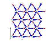
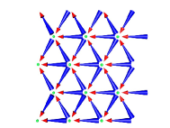
Figure 1: (Color online) Left: A lattice with $L=3$ in its ground-state. The array proposed in this work has six spin in each vertex (small dots). The ice rule is now three in/three out. Right: By applying an strong magnetic field in the $-x$ direction the state shown here should be achieved and by reversing the applied field the system should be driven to the ground-state shown on the left side of the figure.

We have modeled the proposed system by replacing the magnetic moment of each island by a point-like, Ising-like dipole ($\vec{S}_{i}$) that is constrained to point along the line that joins two vertices in the lattice, such that, the interactions are expressed as follows:

$$H_{SI} = Da^{3}\sum_{i\neq j}\left[\frac{\vec{S}_{i}\cdot\vec{S}_{j}}{r_{ij}^{3}}-\frac{3(\vec{S}_{i}\cdot\vec{r}_{ij})(\vec{S}_{j}\cdot\vec{r}_{ij})}{r_{ij}^{5}}\right],$$ (1)

where $D=\mu_{0}\mu^{2}/4\pi a^{3}$ is the dipolar interaction coupling constant, $a$ is the lattice spacing and $\vec{r}_{ij}$ is a vector that connects islands $i$ and $j$. In Fig. 1 we present a sketch of the system, where the vertices and the island’s magnetic moments are shown.

We start our analysis by considering a single vertex and its six spins. It can be easily shown that it is energetically favorable when the moments of a pair of islands are aligned, so that one is pointing into the center of the vertex and the other is pointing out, while it is energetically unfavorable when both moments are pointing inward or both are pointing outward. Therefore the system is expected to be frustrated because for a particular configuration obeying the ice-like rule (three-in/three-out), from the $15$ possible pairs of islands in a vertex, only $9$ can minimize the energy. For the sake of comparison we remember that in the square spin ice there are $6$ pairs at each vertex and only $4$ can minimize the energy when the ice rule is considered.

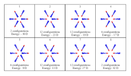
Figure 2: (Color online) The $64$ possible vertices, grouped by increasing energy (left to right) in $8$ topologies. Vertices types 1, 2 and 5 satisfies the three-in/three-out ice rule, while vertices types 3, 4 and 6 are single magnetic charges. Vertices type 7 and 8 are double and triple charged vertices respectively.

Each vertex of the system has $64$ configurations distributed in $8$ different topologies (let us recall that the square lattice has only $16$ configurations distributed in $4$ topologies). In Fig. 2 we show these configurations and topologies, grouped by increasing energy. Types $1,2$ and $5$ obey the three-in/three-out “ice rule”, and analogously to the square lattice, they are energetically split. The remaining types of vertices shown in Fig. 2 possess monopole-like magnetic charges. These correspond to the flip of one, two, or even three spins in a particular vertex. For instance, types $3,4$ and $6$ are monopoles with single charges (with four-in/two-out or two-in/four-out configurations), while types $7$ and $8$ are doubly (five-in/one-out or one-in/five-out) and triply (six-in or six-out) charged monopoles respectively. There are, therefore, $3$ different classes of monopoles with single charge and only one class of doubly and triply charged.

At this point, a fundamental difference between the ASSI and the ATSI appear: while in the ASSI all vertices violating the ice-rule have more energy than the vertices that satisfy it, for the ATSI, this is not true. In an energy scale we have type 1 and type 2 vertices, which satisfies the ice-rule, followed by vertices types 3 and 4, which has four-in/two-out or four-out/two-in spins and of course does not satisfies the ice-rule. Indeed, vertices types 3 and 4 has less energy than type 5 vertices, which has three spins in, three spins out. From this perspective one should expect many differences in the collective behavior of the ATSI and ASSI, for example, in the lowest energy excitations and in the thermodynamic properties; but as will be shown soon they are much more similar than expected.

Going beyond the study of a single vertex we have checked by a simulated annealing process (a Monte Carlo simulation where the system’s temperature is slowly decreased Mol09 ) that the system’s ground-state is indeed composed only by type 1 vertices as can be expected by the vertices energies shown in Fig. 2. Details of the Monte Carlo procedure, including lattice sizes, etc are given in section V. A sketch of the system in its ground-state is shown in Fig. 1.

III Lowest energy excitations

The lowest energy excitation that can be obtained above the ground-state is achieved by flipping one spin, creating two type 4 vertices as shown in Fig 3 (a). This process has an energy cost of approximately $66D$. The second lowest energy state is obtained by flipping a plaquete (Fig. 3 b) and has an energy cost of approximately $77D$. In this case three type 2 vertices are created.

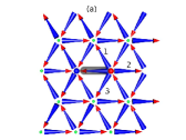
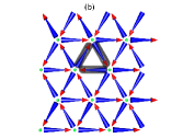
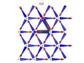
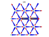
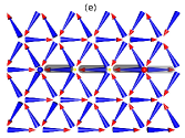
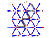
Figure 3: (Color online) (a) Flipping the spin marked in gray results in a monopole anti-monopole pair (big dots). This is the lowest energy excitation of the system. By flipping spins 1, 2 or 3 the configurations of (c) and (d) can be obtained. (b) The second lowest energy state, which is obtained by flipping the marked spins. (c) The third lowest energy state. By repeating this process a sawtooth like string can be formed. (d) The fourth lowest energy state, obtained by flipping the marked spins. (e) A linear string path, where spins marked in dark gray were flipped. By flipping the spin marked in light gray the monopoles are separated by one more lattice spacing. Type 5 vertices that compose the string are marked with small (yellow) dots. (f) A sawtooth string, where spins marked in dark gray were flipped. By flipping the spins marked in light gray the monopoles are separated by one more lattice spacing while the string length increases by two lattice spacings. Type 2 vertices that compose the string are marked with small (green) dots.

Of particular interest is the case where after flipping one spin, which creates two type 4 vertices, more spins are flipped (without further violation of the ice rule) in order to separate them. As can be seen in Fig. 3 (a), to move a excitation to the right side, keeping the neutrality (three-in/three-out) in between, we have three options: flip the spins 1, 2 or 3. By symmetry, its clear that flipping spins 1 or 3 has the same effect in the system and generates the configuration shown in Fig. 3 (c), where a type 2 vertex is created. On the other hand, if spin 2 in Fig. 3 (a) is flipped, the configuration shown in Fig. 3 (d) is formed, which comprises the appearance of a type 5 vertex. As expected, the configuration in Fig. 3 (c) has less energy than the configuration of Fig. 3 (d). While the former costs about $91D$ to be created the latter needs an energy about $123D$. This process can be repeated in order to separate type 4 vertices and the energy of each configuration can be readily obtained, in such a way that we can get the potential energy of the system as a function of the distance between the vertices. Therefore, we have used the same methods of Refs. Mol09, ; Mol10, to determine the potential that better describes the interaction between type 4 vertices. Our results are very similar to those obtained in these references, such that the potential reads:

$$V(R)=q_{t}/R+b_{t}X(R)+c_{t},$$ (2)

where $R$ is the distance between the monopoles and $X(R)$ is the string length.

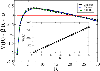
Figure 4: (Color online) Inset: Potential energy as a function of the distance ($R$) between two single charged monopoles separated by a straight string. Outset: The black dots represent the potential minus the linear contribution obtained by fitting $\beta R+\alpha$ to it. The lines are the best non-linear curve fits of the potential according to the functions ($q_{t}/R+b_{t}R+c_{t}$) Coulomb, ($q_{t}\exp(-\kappa R)/R+b_{t}R+c_{t}$) Yukawa and $q_{t}/(R+R_{c})+b_{t}R+c_{t}$ minus $\beta R+\alpha$.

Before showing numerical results some points deserve further explanation. At a first glance, the potential function seems to be linear (see the inset of fig. 4). However, after subtracting from the potential the linear contribution (see fig. 4), one can see that a diverging contribution to the potential for small enough distances must be added to the potential. Among the many possible functions that could be used we found that the addition of a Coulombian term ($q_{t}/R$) to the potential is the best way to describe the ASSI and ATSI data using a function with only three parameters. For the sake of comparison the $\chi^{2}/dof$ is about 0.3 for the pure linear fit and about $6\times 10^{-4}$ for the potential of Eq. 2. Besides that, as can be seen in fig. 4 the potential of Eq. 2 better describes the data. As is well known, one should be very careful when doing a non-linear curve fitting, specially when the fitted function has many parameters, such that the use of functions with more than 3 parameters was avoided. This is the reason why we have opted to describe the excitations by means of Eq. 2. We have also tested other functional forms instead of the Coulomb one, specially the Yukawa potential ($q_{t}\exp(-\kappa R)/R$) and the function $q_{t}/(R+R_{c})$, both with four parameters. Using the Yukawa potential we found approximately the same values for the constants ($q_{t}$, $b_{t}$ and $c_{t}$) and the $\chi^{2}/dof$ diminished by less than one order of magnitude. The use of the $q_{t}/(R+R_{c})$ diminished the $\chi^{2}/dof$ by about one order of magnitude. Nevertheless the fit convergence is highly dependent on the initial values, such that for all purposes we are considering Coulombian interactions between the monopoles. It is worthy noticing that the values shown here are approximate results, that depends on the number of points used in the non-linear fit. Differences up to $20\%$ in $q_{t}$ may be expected.

When single-charged monopoles (type 4 vertices) are separated in a straight line by a straight string, composed by type 5 vertices only (see fig. 3 (e)), the constants in the potential are $q_{t}^{l}=-3.5Da$, $b_{t}^{l}=56D/a$ and $c_{t}^{l}=13D$. The monopoles can also be separated in a straight line by creating only type 2 vertices (see fig. 3 (f)), such that the string has a sawtooth shape. In this case, the constants are $q_{t}^{s}=-3.9Da$, $b_{t}^{s}=25D/a$ and $c_{t}^{s}=46D$, where the string length $X$ is related to the charges distance, $R$, by $X=2R$. The huge difference in the string tension in these situations can be easily understood by recalling that type 2 vertices has less energy than type 5 vertices. It is important to stress that the string in this system is energetic, observable, and unique, in the sense that it is composed by type 2 or type 5 vertices on a background of type 1 vertices. Besides, the value of $q_{t}$ is almost the same of that found in the square spin ice ($-4Da\leq q_{s}\leq-3.4Da$) Mol10 , while the string tension is about six times higher when the string is composed by type 5 vertices only and about two times higher when the string is composed by type 2 vertices ($b_{s}\sim 10D/a$). The difference in the string tension for the shapes considered indicates that there is a huge anisotropy in the system.

IV Ground-state considerations

From an experimental point of view, the achievement of the system’s ground-state is an important step toward the study of monopoles physics. Considering the ATSI we believe that two different approaches can drive the system to its ground-state, or at least to an state close enough to it. The first one is the same approach used by Morgan et al Morgan10 to study the ASSI. In their work they studied the as growth system and found the appearance of ground-state domains with sparse excitations that follows Boltzmann statistics. Considering, for instance, the same island sizes and lattice spacings used by Morgan et al Morgan10 we may expect the achievement of larger domains in the ATSI as compared to the ASSI since in the ATSI, the internal magnetic fields should be stronger. This is by virtue of the presence of more islands in the same area of the material. However, due to experimental difficulties, namely the resolution of the lithography process, it may not be possible to use the same sizes and lattice spacings used by Morgan et al Morgan10 . However, a simpler approach can also be very efficient to drive the system to its ground-state as will be discussed in what follows.

Apply a strong magnetic field in the $-x$ direction of the sample (see Fig. 1), so that the system is driven to the magnetized state shown on the right side of Fig. 1, similarly to what happens to ASSI. However, the energetics of these magnetized configurations, and those deviating from them, are not equivalent in the ASSI and in the ATSI. While the magnetized state of the ASSI is a local minimum, since it is composed by vertices that satisfies the ice rule and any spin flip would increase the system’s energy, in the ATSI the magnetized state is a kind of saddle point. The ATSI’s magnetized state is composed by type 5 vertices only. If a spin in the $x$ direction is flipped, two type 4 vertices are created and since type 4 vertices has less energy than type 5 vertices the system’s energy diminishes. The first spin flipped in the $x$ direction would release an energy of about 45 D. However, if a spin in any other direction is flipped the energy of the system increases since two type 6 vertices are created (remember that type 6 vertices is more energetic than type 5 vertices). If the first spin flipped is not in the $x$ direction, the system’s energy increases by about 10 D. We may thus expect that, after applying a strong field in the $-x$ direction another field applied in the $+x$ direction would induce the formation of type 4 vertices. Once formed, these vertices can be separated apart by creation of type 1 vertices reducing even more the system’s energy. In this process only spins in the $x$ direction (the field direction) are expected to flip. This process would occur in such a way that monopole-like excitations are created above a given state (which is not the ground-state, such that the monopole terminology does not seems to be appropriate) and induced by the presence of the magnetic field to move along the field direction. Note however that south poles (with four-out/two-in) in this situation move in the opposite direction to the field as can be expected by analogy with basic electrostatics. If we restrict our analysis to vertices energy only, we may see that spins that are not in the $x$ direction are not expected to flip, at all, since the vertices that would be created in such a process (type 6) are much more energetic than the other vertices present in the system (types 1, 4 and 5). Even in the presence of a relatively strong disorder the energy needed to flip a spin that is not in the $x$ direction seems to be high enough to prevent its occurrence. However, a detailed analysis of this hypothesis is required due to the long-range character of dipolar interactions. A complete treatment of this possibility is currently in progress and will be published elsewhere.

V Thermodynamics

Knowing the ground state and the elementary excitations, the thermodynamics of the proposed system should deserve attention. Despite the fact that in the artificial spin ices the moment configuration is athermal, some experimental works have presented alternative methods to overcome this difficulty Morgan10 ; Kapaklis11 . Materials with an ordering temperature near room temperature Kapaklis11 are the most recent option; reduction in island’s volume and moment through state-of-the-art nanofabrication is another, but it was not accomplished so far. Besides that, an effective thermodynamic behavior can be obtained by using a rotating magnetic fieldKe08 ; Nisoli07 ; Nisoli10 . Independently of the experimental difficulties we have theoretically studied some thermodynamic properties of the proposed array. Indeed, in an earlier paper considering the ASSI we have argued that the string should loose its tension due to entropic effects Mol09 (the string configurational entropy), rendering free monopoles at a temperature above a critical one, $T_{c}$. The same arguments should be valid here, such that the verification of this hypothesis is of great interest.

To study the thermodynamic properties of this system we have used conventional Monte Carlo techniques, which are briefly presented. We have simulated lattices with size $L\times L_{y}$, where $L_{y}$ is the largest integer resulting from $L/\sqrt{3}$, so that we have $2\times L\times Ly$ vertices and $N_{s}=6\times L\times Ly$ spins for a given $L$; we have considered systems with $L=16,24,32,48,64$ and $80$. Although it is known Mol11 that the introduction of a cut-off radius in the evaluation of dipolar interactions may lead to a critical behavior that does not agree with that found when full long-range interactions are considered, we have opted in this work to use a cut-off radius at eight lattice spacings. This choice is justified by our interest in the basic thermodynamic behavior of the system and not on the details of the possible phase transitions. In our Monte Carlo scheme a combination of single spin flips and loop moves were used. A loop move Barkema98 is a random closed path of aligned spins that are flipped or not according to the Metropolis prescription ($p=\exp{(-\Delta E/k_{B}T)}$). One Monte Carlo step (MCS) is the combination of $N_{s}$ single spin flips and $3$ loop moves. In most simulations we have used $2\times 10^{4}$ MCS to equilibrate the system and $2\times 10^{5}$ MCS to take averages.

We start by presenting the results for the specific heat (see Fig.5). We notice that the specific heat exhibits a peak at a temperature $T_{c}$ approximately equal to $15D/k_{B}$. The amplitude of this peak increases as the system size $L$ increases, as can be seen in the inset of the same figure, where the specific heat maximum is plotted as a function of $\ln(L)$. Therefore, it may indicate a phase transition in the Ising universality class  Privman . We have also analyzed the charges density and the average separation between monopoles and antimonopoles as a function of $T$. In Fig.6 we show the density of single charges (vertices types 3, 4 and 6), $\rho_{1}$, double charges (type 7 vertices), $\rho_{2}$, and triple charges (type 8 vertices), $\rho_{3}$, as a function of temperature. It is remarkable that the density of double and triple charges are much smaller than the density of single charges.

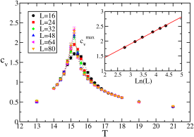
Figure 5: (Color online) Specific heat as a function of temperature for different lattice sizes. The inset shows the specific heat maxima as a function of $\ln(L)$. The line is a guide to the eyes.

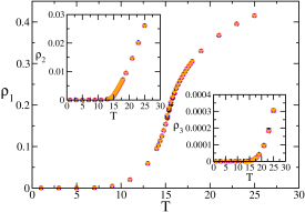
Figure 6: (Color online) Monopoles density as a function of temperature for different lattice sizes. The outer plot shows the density of single charges ($\rho_{1}$) while in the insets the density of double ($\rho_{2}$) and triple ($\rho_{3}$) charges are shown. The symbols are the same used in Fig. 5.

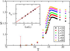
Figure 7: (Color online) Mean distance between single charges as a function of temperature. The inset shows the maximum mean distance as a function of $\ln(L)$. The line is a guide to the eyes.

The mean distance between monopoles and antimonopoles, $S$, as a function of temperature was obtained by considering only defects with unit charge. This quantity is calculated by using the method of assignment problems  Bukard . In our case, we would like to assign $n$ positive charges to $n$ negative charges for a given configuration in such a way that the sum of distances of all possible pairing be a minimum. Note that studying the system’s thermodynamics we are not able to determine the exact pairs energy neither which charge forms a pair with which. The results are shown in Fig.7. The average separation has a local maximum at the same temperature $T_{c}$ in which the specific heat exhibits a peak ($\sim 15D$). We notice that the amplitude of this maximum also increases as the system size increases. Indeed, the maximum average separation $S_{m}$ increases logarithmically with the system size $L$ ($S_{m}\propto\ln L$, see the inset of Fig.7) and hence, one could expect that a certain quantity of monopoles may be almost isolated for very large arrays. For low temperatures the average separation $S$ does not depends on the lattice size $L$, while for high temperatures, this quantity has a tiny dependence on $L$. This picture is suggestive and indicate a different behavior of monopoles and strings at low and high temperatures Mol09 ; Silva12 .

At this point we should stress that the similarities between these results and the results for the ASSI of Ref. Silva12 are remarkable. As discussed before one would expect many differences between those systems since some vertices that does not satisfy the ice rule have less energy than some vertices that satisfy it. Indeed, the fact that the some of the vertices of a string (type 5) have more energy than two kinds of charges (vertices types 3 and 4) would be expected to considerably change the system’s properties, specially those concerning monopoles behavior. However, the only difference that can be noticed is in the critical temperature, which is about $15D/k_{B}$ for the ATSI and $7D/k_{B}$ for the ASSI. The specific heat and magnetic charge behaviors are qualitatively the same, including the mean distance between opposite magnetic charges and their finite size behavior. Of course, as the string in the ATSI has stronger tension, the maximum value of the mean distance between the monopoles is smaller than that of the ASSI for the same lattice size.

VI Conclusions

In summary, we have proposed and theoretically studied a realization of an artificial spin ice in a triangular geometry. The usual experimental difficulty to achieve the ground-state of the artificial square spin ice (ASSI) should not be so dramatic for the artificial triangular spin ice (ATSI) array since a simple demagnetization protocol (similar to a hysteresis loop) will probably drive the system to its ground-state as discussed in section IV (see Fig. 1). This hypothesis is under current investigation. Although there are fundamental differences between the ASSI and the ATSI, specially concerning the vertices topologies, these systems show remarkable similarities. Indeed, the lowest energy excitations of both can be described by magnetic monopoles excitations interacting via a Coulombic term added by an energetic string potential; the thermodynamic behaviors are qualitatively the same. However, contrary to the ASSI, in the ATSI there are 3 different classes of magnetic monopoles, and much more work has to be done to completely understand if all kinds of charged vertices behave in the same way. The same applies for the different classes of three-in/three-out vertices.

Another issue that deserves further investigation is the similarity found in the monopoles’ charge value. While the string tension of the ATSI can be about six times larger than that of the ASSI, the monopoles’ charge have roughly the same value. Indeed, in Ref. Mol10, we have shown that in a modified ASSI, where a height off-set is introduced between the islands in the two different lattice directions, the string tension can be reduced by a factor of about 20 and the monopoles’ charge does not change appreciably. For example, the smallest value of the string tension found for the modified ASSI is about $0.59D/a$ and the highest value we found in this study is $56D/a$ which gives a difference of about 2 orders of magnitude. In general, we expect that the value of the string tension $b$ will not alter the physical picture of artificial systems with different geometries; it must only change the thermodynamic quantities, and $T_{c}$ should increase as $b$ increases (for instance, square and triangular lattices present similar thermodynamic properties but $T_{c}$ is lower in the square lattice, which has smaller $b$). Remember that following our arguments on energy-entropy balance in ASSI Mol09 we found that the effective string tension should be given by $b-\epsilon k_{B}T$, with $\epsilon=\mathcal{O}(a^{-1})$. In this way the critical temperature, the temperature at which the string looses its effective tension, is proportional to the string tension $b$. Of course, $T_{c}\rightarrow 0$ if $b\rightarrow 0$ and hence, magnetic monopoles would be found free for any temperature. Besides, it is expected that smaller string tension demands a weaker field to move the monopoles. On the other hand, all monopoles’ charge values are in the range $-4Da\leq q\leq-3.4Da$ Mol10 . This observation may indicate that these charges have a kind of universal behavior while the string tension can be tuned by modifying the system’s geometry. In addition, it is expected that whenever controlling the monopoles motion, spin ice systems could be used for several practical applications. Indeed, the ability of designing systems with desired string tension, concerned to the field necessary to move a charge, would benefit the development of new devices. The main challenge should be then to find geometries in two-dimensions (or even in three dimensions  Moller09 ; Mol10 ) in which $b\sim 0$ making the control of monopole excitations experimentally feasible by means of externally applied magnetic fields. Of course, a great deal of efforts must be done in order to verify the validity and applicability of these assumptions.

Another prospect for future investigation is the searching for a three-dimensional natural version of this system, a hypothetical “bulk spin ice” with three-in/three-out ice rule. In this case, the expected crystalline structure would be composed by Ising-like spins (as in Dy₂Ti₂O₇ and Ho₂Ti₂O₇) disposed in a network of linked octahedra (which represents the central intersection of two tetrahedra) in such a way that they are constrained to point along the line joining the center of adjacent octahedra.

The authors thank CNPq, FAPEMIG, FUNARBE and CAPES (Brazilian agencies) for financial support.

References

- (1) C. Castelnovo, R. Moessner, and L. Sondhi, Nature 451, 42 (2008).
- (2) T. Fennell et al., Science 326, 415 (2009).
- (3) D.J. P. Morris et al., Science 326, 411 (2009).
- (4) S.T. Bramwell et al., Nature 461, 956 (2009).
- (5) H. Kadowaki et al., J. Phys. Soc. Jpn. 78, 103706 (2009).
- (6) L.D.C. Jaubert and P.C.W. Holdsworth, Nature Phys. 5, 258 (2009).
- (7) S.R. Giblin et al., Nature Phys. 7, 252 (2011).
- (8) S. Ladak et al., Nature Phys. 6, 359 (2010).
- (9) R.F. Wang et al., Nature 439, 303 (2006).
- (10) J. Li et al., Phys. Rev. B 81, 092406 (2010).
- (11) H. Zabel, A. Schumann, W. Westphalen, and A. Remhof, Acta Phys. Pol. A 115, 59 (2009).
- (12) E. Mengotti et al., Nature Phys. 7, 68 (2011).
- (13) Y. Nambu, Nucl. Phys. 130, 505 (1977).
- (14) L.A. Mól et al., J. Appl. Phys. 106, 063913 (2009).
- (15) L.A.S. Mól, W.A. Moura-Melo, and A.R. Pereira, Phys. Rev. B 82, 054434 (2010).
- (16) J.P. Morgan, A. Stein, S. Langridge, and C. Marrows, Nature Phys. 7, 75 (2011).
- (17) G. Möller and R. Moessner, Phys. Rev. B 80, 140409(R) (2009).
- (18) G. Möller and R. Moessner, Phys. Rev. Lett. 96, 237202 (2006).
- (19) R.C. Silva, F.S. Nascimento, L.A.S. Mól, W.A. Moura-Melo, and A.R. Pereira, New Journal of Physics 14, 015008 (2012).
- (20) Z. Budrikis, P. Politi, and R.L. Stamps, Phys. Rev. Lett. 105, 017201 (2010).
- (21) V. Kapaklis et al., New Journal of Physics 14, 035009 (2012).
- (22) X. Ke et al., Phys. Rev. Lett. 101, 037205 (2008).
- (23) C. Nisoli et al., Phys. Rev. Lett.98, 217203 (2007).
- (24) C. Nisoli et al., Phys. Rev. Lett. 105, 047205 (2010).
- (25) L.A.S. Mól and B.V. Costa, ArXiv: 1109.1840, cond.mat (2011).
- (26) G.T. Barkema and M.E.J. Newman, Phys. Rev. E 57, 1155 (1998).
- (27) V. Privman (Ed.) “Finite Size Scaling and Numerical Simulation of Statistical Systems.” World Scientific, 1990.
- (28) R. Bukard, M. Dell‘Amico, and S. Martello, Assignment Problems (Society for Industrial and Applied Mathematics, Philadelphia, 2009).