Methods to distinguish between polynomial and exponential tails

Resum

In this article two methods to distinguish between polynomial and exponential tails are introduced. The methods are mainly based on the properties of the residual coefficient of variation for the exponential and non-exponential distributions. A graphical method, called CV-plot, shows departures from exponentiality in the tails. It is, in fact, the empirical coefficient of variation of the conditional excedance over a threshold. The plot is applied to the daily log-returns of exchange rates of US dollar and Japan yen.

New statistics are introduced for testing the exponentiality of tails using multiple thresholds. Some simulation studies present the critical points and compare them with the corresponding asymptotic critical points. Moreover, the powers of new statistics have been compared with the powers of some others statistics for different sample size.

Keywords:

Residual coefficient of variation. Multiple testing problem. Heavy tailed distributions. Power distributions. Extreme value theory.

1 Introduction

Since Balkema-DeHaan (1974) and Pickands (1975), it has been well known that the conditional distribution of any random variable over a high threshold — what is known in reliability as the residual life — has approximately a generalized Pareto distribution (GPD). The exponential distribution is a particular case that appears between compact support distributions and heavy-tailed distributions, in GPD. Applications of extreme value theory to risk management in finance and economics are now of increasing importance. The GPD has been used by many authors to model excedances in several fields such as hydrology, insurance, finance and environmental science, see McNeil et al. (2005), Finkenstadt and Rootzén (2003), Coles (2001) and Embrechts et al. (1997).

It is especially important for applications to distinguish between polynomial and exponential tails. Often, the methodology is based on graphical methods to determine the threshold where the tail begins, see Embrechts et al. (1997) and Ghosh and Resnick (2010). In this cases, multiple testing problem occurs when one considers a wide set of thresholds.

The main objective of this paper is providing ways to distinguish the behavior of tails, avoiding the multiple testing problems. The methods are mainly based on the properties of the residual coefficient of variation that is closely related to the likelihood functions of the exponential and Pareto distributions, see Castillo and Puig (1999) and Castillo and Daoudi (2009). The empirical coefficient of variation, or equivalent statistics (e.g., Greenwood’s statistic, Stephens $W_{s}$) are omnibus tests used for testing exponentiality against arbitrary increasing failure rate or decreasing failure rate alternatives. A good description of these tests has been given by D’Agostino and Stephens (1986).

A large number of tests for exponentiality have been proposed in the literature. Montfort and Witter (1985) propose the maximum/median statistic for testing exponentiality against GPD. Smith (1975) and Gel, Miao and Gastwirth (2007) show that powerful tests of normality against heavy-tailed alternatives  are obtained using the average absolute deviation from the median. Lee et al. (1980) and Ascher (1990) discuss tests based on the equation $E\left(X^{p}\right)/E\left(X\right)^{p}=\Gamma\left(1+p\right)$, for some $p>0$, where $X$ is an exponential random variable. The limit case, when $p$ tends to $0$, is studied in Mimoto and Zitikis (2008), see also references therein. The case $p=2$ is equivalent to the coefficient of variation test. Lee et al. (1980) show that in this case the power is poor testing against distributions whose coefficient of variation is $1$ (the exponential case) as happens testing against the absolute values of the Student distribution $t_{4}$. Our methods based on a multivariate point of view are also useful in this situation, since the exponential distribution is the unique distribution with the residual coefficient of variation over any threshold equal to $1$; see Sullo and Rutherford (1977), Gupta (1987) and Gupta and Kirmani (2000).

In Section 2 the asymptotic distribution of the residual coefficient of variation is studied as a random process in terms of the threshold. This provides a clear graphical method, called a CV-plot, for assessing departures from exponentiality in the tails. The qualitative behavior of the CV-plot is made more precise in Section 3. The plot is applied to the daily log-returns of exchange rates of US dollar and Japan yen.

New statistics are introduced for testing the exponentiality of tails using multiple thresholds in Section 4. Some simulation studies present the critical points and compare them with the corresponding asymptotic critical points.

In Section 5, the powers of new statistics have been compared with the powers of some others statistics against heavy-tailed alternatives, given by Pareto and absolute values of the Student distributions, for different sample size.

2 The residual coefficient of variation

Let $X$ be a continuous non negative random variable with distribution function $F\left(x\right)$. For any threshold, $t>0$, the distribution function of threshold excedances, $\left(X-t\mid X>t\right)$, denoted $F_{t}\left(x\right)$, is defined by

$$1-F_{t}\left(x\right)=\frac{1-F\left(x+t\right)}{1-F\left(t\right)}.$$

The coefficient of variation (CV) of the conditional excedance over a threshold, $t$, (the residual CV) is

$$CV\left(t\right)=Var\left(X-t\mid X>t\right)^{1/2}/E\left(X-t\mid X>t\right)$$

where $E\left[\cdot\right]$ and $\ Var\left[\cdot\right]$ denote the expected value and the variance. The $CV\left(t\right)$ is independent of scale parameters. It will be useful find the distribution of the empirical $CV$ process for all values of $t$.

It is well known that the mean residual lifetime determines the distribution for random variables. Gupta and Kirmani (2000) showed that mean residual life is a function of the residual coefficient of variation, hence it also characterize the distribution. In this context, generalized Pareto distributions appear as the simple case in which the residual coefficient of variation is a constant. Hence, from Pickands (1975) and Balkema-DeHaan (1974), it is almost constant for a sufficiently high threshold.

Denote $X1_{\left(X>t\right)}$ the random variable $X$ if it is larger that $t$ and zero otherwise. Denote $\mu_{0}\left(t\right)=\Pr\left\{X>t\right\}$ and $\mu_{k}\left(t\right)=E\left[X^{k}1_{\left(X>t\right)}\right]$, $k>0$. Throughout this paper $\mu_{0}\left(t\right)>0,$ foll all $t$, is assumed. Note that

$$\mu_{k}\left(t\right)=\mu_{0}\left(t\right)E\left(X^{k}\mid X>t\right).$$

Given a sample $\left\{X_{j}\right\}$ of size $n$, let $n\left(t\right)=\sum_{j=1}^{n}1_{\left(X_{j}>t\right)}$ the number of excedance over a threshold, $t$. By the law of large numbers, $n\left(t\right)/n$ converges to $\mu_{0}\left(t\right)$. The empirical CV of the conditional excedance is given by

$$cv_{n}\left(t\right)=\frac{n\left(t\right)}{\sum_{j=1}^{n}\left(X_{j}-t\right)1_{\left(X_{j}>t\right)}}\times\\ \left[\frac{\sum_{j=1}^{n}X_{j}^{2}1_{\left(X_{j}>t\right)}}{n\left(t\right)}-\left(\frac{\sum_{j=1}^{n}X_{j}1_{\left(X_{j}>t\right)}}{n\left(t\right)}\right)^{2}\right]^{1/2}$$ (1)

The $cv_{n}\left(t\right)$ is also independent of scale parameters, since the mean and standard deviation have the same units.

Proposition 1

The $cv_{n}\left(t\right)$ is a consistent estimator of $CV\left(t\right)$, assuming finite second moment, since the limit in probability of $cv_{n}\left(t\right)$, as $n$ goes to infinity is

$$m_{cv}\left(t\right)=\frac{\sqrt{\mu_{2}\left(t\right)\mu_{0}\left(t\right)-\mu_{1}\left(t\right)^{2}}}{\mu_{1}\left(t\right)-t\mu_{0}\left(t\right)}=CV\left(t\right)$$

Proof. Fixed $t$, as $n$ goes to infinity

$$\frac{1}{n\left(t\right)}\sum_{j=1}^{n}X_{j}^{k}1_{\left(X_{j}>t\right)}=\frac{n}{n\left(t\right)}\frac{1}{n}\sum_{j=1}^{n}X_{j}^{k}1_{\left(X_{j}>t\right)}\rightarrow\mu_{k}\left(t\right)/\mu_{0}\left(t\right)=E\left[X^{k}\mid X>t\right],$$

by the law of large numbers. Hence, the limit in probability of $cv_{n}\left(t\right)$ is

$$\frac{\sqrt{\mu_{2}\left(t\right)/\mu_{0}\left(t\right)-\left(\mu_{1}\left(t\right)/\mu_{0}\left(t\right)\right)^{2}}}{\mu_{1}\left(t\right)/\mu_{0}\left(t\right)-t}=\frac{\sqrt{Var\left(X-t\mid X>t\right)}}{E\left(X-t\mid X>t\right)}$$

 

Let us define the standardized $k$-th sampling moment of the conditional excedance by

$$W_{k,n}\left(t\right)=\frac{1}{\sqrt{n}}\sum_{j=1}^{n}\left\{X_{j}^{k}1_{\left(X_{j}>t\right)}-\mu_{k}\left(t\right)\right\},$$

hence,

$$\sum_{j=1}^{n}X_{j}^{k}1_{\left(X_{j}>t\right)}=\sqrt{n}W_{k,n}\left(t\right)+n\mu_{k}\left(t\right).$$ (2)

Note that normalizing constant $1/\sqrt{n}$ is used in order to have $W_{k,n}\left(t\right)=O_{p}\left(1\right)$, with orders of convergence in probability notation. The covariance of this random process is given by

$$cov\left(W_{i,n}\left(s\right),W_{j,n}\left(t\right)\right) =cov\left(X^{i}1_{\left(X>s\right)},X^{j}1_{\left(X>t\right)}\right)$$

$$=\mu_{i+j}\left(s\vee t\right)-\mu_{i}\left(s\right)\mu_{j}\left(t\right),$$ (3)

Throughout this paper the quantities $cv$ and $W_{k}$ among others depend on $n$;  wherever possible the dependence of quantities on $n$ is suppressed for simplicity. Even the dependence on $t$ is dropped for $W_{k}=W_{k}\left(t\right)$ and $\mu_{k}=\mu_{k}\left(t\right)$, in many places.

Theorem 2

Let $X$ be a continuous non negative random variable with finite fourth moment. Then, the following expansion holds

$$\sqrt{n}\left(cv\left(t\right)-m_{cv}\left(t\right)\right)\! \!\!=\!\! \!\frac{\mu_{0}W_{2}}{2\left(\mu_{1}-t\mu_{0}\right)\!\sqrt{\mu_{2}\mu_{0}-\mu_{1}^{2}}}+\frac{\mu_{0}\left(t\mu_{1}-\mu_{2}\right)W_{1}}{\left(\mu_{1}-t\mu_{0}\right)^{2}\!\sqrt{\mu_{2}\mu_{0}-\mu_{1}^{2}}}+\!$$

$$+\frac{\left(-2t\mu_{1}^{2}+t\mu_{0}\mu_{2}+\mu_{1}\mu_{2}\right)W_{0}}{2\left(\mu_{1}-t\mu_{0}\right)^{2}\sqrt{\mu_{2}\mu_{0}-\mu_{1}^{2}}}+O_{p}\left(\frac{1}{\sqrt{n}}\right).$$

Proof. The expression $\left(\ref{cv1}\right)$ in terms of $W_{k}=W_{k,n}\left(t\right)$ is

$$cv\left(t\right)=\frac{\mu_{0}\left(t\right)+W_{0}/\sqrt{n}}{\mu_{1}\left(t\right)+W_{1}/\sqrt{n}-t\left(\mu_{0}\left(t\right)+W_{0}/\sqrt{n}\right)}\times\\ \left[\frac{\mu_{2}\left(t\right)+W_{2}/\sqrt{n}}{\mu_{0}\left(t\right)+W_{0}/\sqrt{n}}-\left(\frac{\mu_{1}\left(t\right)+W_{1}/\sqrt{n}}{\mu_{0}\left(t\right)+W_{0}/\sqrt{n}}\right)^{2}\right]^{1/2}$$ (5)

Let $w_{k}=W_{k}/\sqrt{n}=O_{p}\left(1/\sqrt{n}\right)$, since $W_{k}=O_{p}\left(1\right).$ Then, let us replace $w_{k}$ in $\left(\ref{cv3}\right)$. Taking a Taylor expansion of $\sqrt{n}\left(cv\left(t\right)-m_{cv}\left(t\right)\right)$ with respect to $w_{k}$ near zero the result follows.   

Example 3

Let $X$ be a random variable with an exponential distribution with mean $\mu$. Conditional moments of $X$, $\mu_{k}\left(t\right)$, can be obtained from the conditional moments of the exponential distribution of mean $1,\mu_{k}^{1}\left(t\right)$ by

$$\mu_{k}\left(t\right)=\mu^{k}\mu_{k}^{1}\left(t/\mu\right)$$

where

$$\mu_{0}^{1}\left(t\right) \!\!\!\!=\!\!\!\! e^{-t},\qquad\mu_{1}^{1}\left(t\right)=e^{-t}\left(1+t\right),\qquad\mu_{2}^{1}\left(t\right)=e^{-t}\left(2+t\left(2+t\right)\right)$$

$$\mu_{3}^{1}\left(t\right) \!\!\!\!=\!\!\!\! e^{-t}\left(6+t\left(6+t\left(3+t\right)\right)\right),\,\mu_{4}^{1}\left(t\right)=e^{-t}\left(24+t\left(24+t\left(12+t\left(4+t\right)\right)\right)\right).$$

In particular

$$m_{cv}\left(t\right)=1.$$

In this Section several results on the convergence of random processes are shown, in the sense of convergence of finite-dimensional distributions. These results are sufficient for the applications given in Section 4.

If tightness is proved then weak convergence in the Skorokhod space follows, but this will not be considered here.

Corollary 4

Let $X$ be a random variable with exponential distribution of mean $\mu$; then $\sqrt{n}\left(cv\left(t\right)-1\right)$ converges to a Gaussian process with zero mean and covariance function given by

$$\rho\left(s,t\right)=\exp\left(\frac{s\wedge t}{\mu}\right)\text{.}$$

In particular

$$\sqrt{n}\left(cv\left(0\right)-1\right)\overset{d}{\rightarrow}N\left(0,1\right)\text{,}$$ (6)

that corresponds to the asymptotic distribution of Greenwood’s statistic.

Proof. From Theorem 2 and Example 3 it follows that

$$\sqrt{n}\left(cv\left(t\right)-1\right)=\left(W_{0},W_{1},W_{2}\right)\ a\left(t\right)+O_{p}\left(n^{-1/2}\right)$$

where

$$a\left(t\right)^{\prime}=(e^{t/\mu}\,\left(t^{2}+4\,t\,\mu+2\,{\mu}^{2}\right)/\left(2\,{\mu}^{2}\right),-e^{t/\mu}\,\left(t+2\,\mu\right)/{\mu}^{2},e^{t/\mu}/\left(2\,{\mu}^{2}\right))$$

Then, the covariance matrix of $W=\left(W_{0},W_{1},W_{2}\right)^{\prime}$, from $\left(\ref{cov}\right)$ and Example 3, assuming $s\leq t$, is

$$\mathrm{cov}\left(W(s),W(t)\right)\equiv M\left(s,t\right)=\left(\mu_{i+j}\left(t\right)-\mu_{i}\left(s\right)\mu_{j}\left(t\right)\right)_{i,j=0,1,2}.$$

Some algebra shows

$$a\left(s\right)^{\prime}M\left(s,t\right)\ a\left(t\right)=\exp\left(s/\mu\right).$$

 

Proposition 5

Let $X$ be a random variable with exponential distribution of mean $\mu$; then using a new time scale, $\tau=\mu\log t$, for $t\geq 1$, the random process of $\sqrt{n}\left(cv\left(\tau\right)-1\right)$ converges to standard Brownian Motion.

Proof. From $\left(\ref{c1}\right)$, given $s,t\geq 1$,

$$\rho\left(\mu\log s,\mu\log t\right)=\exp\left(\log s\wedge\log t\right)=s\wedge t$$

 

Corollary 4 uses the same $n$ in $\sqrt{n}\left(cv\left(t\right)-1\right)$ for all $t$. The next result uses the sample size adapted to the corresponding $t$.

Corollary 6

Let $X$ be a random variable with an exponential distribution, then $\sqrt{n\left(t\right)}\left(cv\left(t\right)-1\right)$ converges to a Gaussian process with zero mean and covariance function given by

$$\exp\left(-\left|s-t\right|/\left(2\mu\right)\right).$$

This is the covariance function of the Ornstein-Uhlenbeck process, the continuous time version of an $AR(1)$ process. It is a stationary Markov Gaussian process. In particular, for any fixed $t$

$$\sqrt{n\left(t\right)}\left(cv\left(t\right)-1\right)\overset{d}{\rightarrow}N\left(0,1\right)\text{.}$$ (7)

Proof. We remember that $n\left(t\right)/n$ converges to $\mu_{0}\left(t\right)=\Pr\left\{X>t\right\}>0$. Hence, if $n$ tends to infinity $n(t)$ tends to infinity too.We can write

$$\sqrt{n\left(t\right)}\left(cv\left(t\right)-1\right)=\sqrt{n\left(t\right)/n}\sqrt{n}\left(cv\left(t\right)-1\right).$$

From $\left(\ref{as}\right)$ and Example 3, we have

$$\frac{n\left(t\right)}{n}=\exp\left(-t/\mu\right)+\frac{W_{0}}{\sqrt{n}}.$$

Then $\sqrt{n\left(t\right)}\approx\sqrt{n}\exp\left(-t/2\mu\right)$ and we have that

$$\exp\left(-s/2\mu\right)\exp\left(\frac{s\wedge t}{\mu}\right)\exp\left(-t/2\mu\right)=\exp\left(-\left|s-t\right|/\left(2\mu\right)\right).$$

 

3 CV-plot

Given a sample $\left\{x_{k}\right\}$ of positive numbers of size $n$, we denote by $\left\{x_{\left(k\right)}\right\}$ the ordered sample, so that $x_{\left(1\right)}\leq x_{\left(2\right)}\leq...\leq x_{\left(n\right)}$. We denote by CV-plot the representation of the empirical CV of the conditional excedance $\left(\ref{cv1}\right)$, given by

$$k\rightarrow cv\left(x_{\left(k\right)}\right)\text{.}$$ (8)

The CV-plot does not depend on scale parameters, since the $cv_{n}\left(t\right)$ does not. That is, the CV-plots for samples $\left\{x_{k}\right\}$ and $\left\{\lambda\ x_{k}\right\}$ are the same, for any $\lambda>0$.  In order to have a reference for the behavior of $\left(\ref{plot1}\right)$, pointwise error limits for these plots can be obtained for large samples using $\left(\ref{ex}\right)$, from the null hypothesis of exponentiality. In Section 4, pointwise error limits of the CV-plot are computed by simulation for samples of several sizes. Then, the points are joined by linear interpolation and plotted in the CV-plots.

Under regularity conditions, the conditional distribution of any random variable over a high threshold is approximately GPD and this model is characterized as the family of distributions with constant residual CV, as has been said. Hence, the CV-plot can be a complement tool to the Hill-plot or the ME-plot, which are used as diagnostics in the extreme values theory, see Ghosh and Resnick (2010).

In order to illustrate the usefulness of the residual coefficient of variation, we are going to examine the behavior of exchange rates between the US dollar and the Japanese yen (JPY), from January 1, 1979 to December 31, 2003. The data set is available from OANDA Corporation at http://www.oanda.com/ convert/fxhistory.

The daily returns for the dollar price, $P_{k}$, are given by

$$x_{k}=\log\left(P_{k}\right)-\log\left(P_{k-1}\right)$$

The daily returns are assumed to be independent here, as in the most basic financial models. However, the theory may be extended even for short-range correlations, see Coles (2001, chap. 5)

The set of positive returns is called the positive part of returns and  the set of minus the negative returns is called the negative part. Both cases are samples of positive random variables. From the 25 years considered we have 9131 daily returns, 3840 of which are positive, 3642 negative and 1649 are equal to zero.

In Figure 1, the plots (a) and (b) are the CV-plots of the $n=2000$ largest values for the positive and negative part of dollar/yen returns, respectively. Pointwise 90% limits around the line $cv=1$ are included, the lowest sample size we consider is $20$, since not relevant information comes from smaller samples. Since the basic model for returns is the normal distribution, we will assume that the distribution has support in $(0,\infty)$.  Then, their threshold excedances, for large thresholds, are very nearly Pareto distributed with parameter $\xi>0$ (Pickands, 1975). Some remarks arise from Figure 1. The plot (a) shows that the process $\left(\ref{plot1}\right)$ for the positive part of dollar/yen returns is always inside the pointwise limits for the exponential distribution. Moreover, since we are only interested to test against Pareto alternatives, we have to consider only upper bounds; thus the pointwise level is $95\%$. Hence, the hypothesis that $CV=1$ can be accepted and we can say that the tails decrease at an exponential rate. Note that use of simultaneous confidence limits would make the bounds wider, reinforcing our conclusion.

The plot (b) shows that the process $\left(\ref{plot1}\right)$ for the negative part of dollar/yen returns is clearly outside the error limits for the exponential distribution in most of the range. It seems clear that we have to reject the hypothesis of exponentiality. However, the coefficient of variations looks like a constant, approximately. Hence, a Pareto distribution might be accepted for the sample.

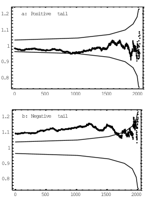
Figura 1: The plots (a) and (b) are the CV-plots of the $n=2000$ largest values for the positive and negative parts of dollar/yen returns, respectively, with pointwise 90% error limits under the exponential distribution hypothesis.

4 Testing exponentiality allowing multiple thresholds

The CV-plot, explained in the last subsection, provides a clear graphical method for assessing departures from exponentiality in the tails. This qualitative behavior shall be made more precise here by introducing new tests of exponential tails adapted to the present situation. The tests are more powerful than most tests against the absolute values of the Student distribution, as we will see in Section 5, including the empirical coefficient of variation, or equivalent statistics as Greenwood’s statistic or Stephens $W_{s}$ (D’Agostino and Stephens, 1986). Our approach is the following:

Given a sample $\left\{x_{j}\right\}$ from an exponential distribution, for any set of thresholds $t_{0}<t_{1}<...<t_{m}$, let $n\left(t_{k}\right)$ be the number of events in $\left\{x_{j}:x_{j}>t_{k}\right\}$, and $cv\left(t_{k}\right)$ the empirical CV given by $\left(\ref{cv1}\right)$, where $0\leq k\leq m$.

From $\left(\ref{ex}\right)$, asymptotically $n\left(t_{k}\right)\left(cv\left(t_{k}\right)-1\right)^{2}$ is distributed as a $\chi_{1}^{2}$ distribution. Let us consider the statistic

$$T=\sum_{k=0}^{m}n\left(t_{k}\right)\left(cv\left(t_{k}\right)-1\right)^{2}.$$ (9)

Clearly the asymptotic expectation of $T$ is $m+1$; however, its asymptotic distribution is not $\chi_{m+1}^{2}$, since the random variables $cv\left(t_{k}\right)$ are not independent. Its distribution does not depend on scale parameters and it is straightforward to simulate the distribution of $T$. It is important to note that lower values for $T$ are expected under the null hypothesis of exponentiality, when the expected values for $cv\left(t_{k}\right)$ are $1$. Hence, high values for $T$ show departure from exponential tails.

The thresholds $\left\{t_{k}\right\}$ can be arbitrary but some practical simplicity is obtained by taking thresholds approximately equally spaced, under the null hypothesis of exponentiality. The next result shows a way of doing this.

Proposition 7

If $X$ is a random variable with exponential distribution of mean $\mu$, then

$$\Pr\left\{X>\left(\mu\log 2\right)k\right\}=1/2^{k}$$

Given a sample $\left\{x_{j}\right\}$ of size $n$ with exponential distribution, the subsample of the last $n/2^{k}$ elements (assuming that $n/2^{k}$ is integer) corresponds to the elements greater than the order statistic $x_{\left(n-n/2^{k}\right)}$ and $x_{\left(0\right)}=0$, $x_{\left(n/2\right)}$, $x_{\left(3\ n/4\right)}$, $x_{\left(7\ n/8\right)}$, … are approximately equally spaced, from Proposition 7.

For a general sample, the quantiles $q_{k}$ corresponding to the last $n/2^{k}$ elements are considered $(q_{1}$ is the median, $q_{2}$ is the third quartile, …$)$. From $\left(\ref{p4}\right)$, $q_{k}\approx\left(\mu\log 2\right)k\approx x_{\left(n-n/2^{k}\right)}$. Taking the set of thresholds corresponding to these sampling quantiles, $\left(\ref{cd0}\right)$ became

$$T_{m}=n\sum_{k=0}^{m}2^{-k}\left(cv\left(q_{k}\right)-1\right)^{2}$$ (10)

4.1 Asymptotic distribution

It is possible to write $\left(\ref{cd}\right)$ in the form $T_{m}$ $=V^{\prime}V$, where

$$V^{\prime}=\sqrt{n}\left[cv\left(q_{0}\right)-1,2^{-1/2}\left(cv\left(q_{1}\right)-1\right),...,2^{-m/2}(cv\left(q_{m}\right)-1)\right]$$

The asymptotic distribution of $T_{m}$ can be found from Corollary 4 in the following way. From Proposition $\ref{p4},$ we have that $q_{k}\approx\left(\mu\log 2\right)k$. Then, asymptotically, the covariance matrix for $V$ is

$$\Sigma_{m}=\left(2^{-i/2}\rho\left(q_{i},q_{j}\right)2^{-j/2}\right)_{i,j=0,...,m}=\left(2^{-\left|i-j\right|/2}\right)_{i,j=0,...,m}$$

Theorem 8

The asymptotic distribution of $T_{m}$ is $\sum_{0}^{m}\lambda_{i}Z_{i}^{2}$ with $Z_{i}$ distributed as independent $N(0,1)$ and $\lambda_{i}$ the eigenvalues of $\Sigma_{m}$.

Proof. From the central limit theorem $V$ is asymptotically multivariate normal $N\left(0,\Sigma_{m}\right)$. Then, in a classical argument, $\Sigma_{m}=A\ \Lambda\ A^{\prime}$ with $A$ an orthogonal matrix and $\Lambda$ the diagonal matrix of the eigenvalues. It follows that $V=A\ \Lambda^{1/2}Z$ with $Z$ asymptotically multivariate normal with the identity as covariance matrix, $N\left(0,I\right)$. Then $T_{m}$ $=V^{\prime}V=Z^{\prime}\Lambda\ Z=\sum_{0}^{m}\lambda_{i}Z_{i}^{2}$, because $A$ is an orthogonal matrix.   

Example 9

For instance, for $m=2$,

$$\Sigma_{2}=\left(\begin{array}[]{ccc}1&1/\sqrt{2}&1/2\\ 1/\sqrt{2}&1&1/\sqrt{2}\\ 1/2&1/\sqrt{2}&1\end{array}\right)$$

and the eigenvalues are given by

$$\lambda_{0}=\left(5+\sqrt{17}\right)/4,\lambda_{1}=1/2,\lambda_{2}=\left(5-\sqrt{17}\right)/4$$

Note also that for $m=0$, the asymptotic distribution of $T_{0}$ is simply a $\chi_{1}^{2}$ distribution. Numerical values of the eigenvalues $\lambda_{i}$ are given in Table 1 for other small values of $m$.

4.2 Approximate critical points

Simulation methods are now easily available to compute critical values and p-values of $T_{m}$. However, the asymptotic distribution of $T_{m}$, given by Theorem 8, provides a way to compute such p-values for large sample sizes without heavy simulation. For instance, if the sample size is $n=2000$ and $m=3$, the direct method needs samples of $2000$ exponential random numbers and the asymptotic distribution only needs samples of $4$ normal random numbers.

Moreover, the asymptotic distribution of $T_{m}$, given by Theorem 8, can be approximated by $a+b\chi_{\nu}^{2}$, where $\chi_{\nu}^{2}$ has gamma distribution with parameters $\left(\nu/2,2\right)$, fitting the constants $a,b,\nu$ in order the three first moments of $\sum_{0}^{m}\lambda_{i}Z_{i}^{2}$ and $a+b\chi_{\nu}^{2}$ be equal. This leads us to solve:

$$a+b\ \nu=\sum_{0}^{m}\lambda_{i},\quad b^{2}\nu=\sum_{0}^{m}\lambda_{i}^{2},\quad b^{3}\nu=\sum_{0}^{m}\lambda_{i}^{3}$$ (11)

Table 1 shows the eigenvalues of the asymptotic covariance matrix of $T_{m}$ and the corresponding constants, $a$, $b$, and $\nu$ for $m=1,2,3$ and $4$.

Table 2 shows the critical points, obtained by simulation, for the $T_{m}$ statistics ($m=0,1,2,3$ and $4$) for samples of size $50$, $100$, $200$, $500$, $1000$ and $2000$, corresponding to the $90$, $95$ and $99$ percentiles, as well as the values obtained by simulation of the asymptotic distribution $\left(\ref{p3}\right)$ and the approximation given from $\left(\ref{app}\right)$. The simulations are all run with $50,000$ samples. It can be seen that the asymptotic and approximate methods are useful for samples larger than $500$. These two methods are particularly useful for finding rough p-values. Note that for the approximate method,

$$\Pr\left\{T_{m}>t\right\}=\Pr\left\{\chi_{\nu}^{2}>(t-a)/b\right\}$$

where $a,b,\nu$ are the solutions of $\left(\ref{app}\right)$.

$$\begin{array}[]{|c|c|c|c|c|c|c|c|c|}\hline\cr&\vrule\lx@intercol\hfil\text{EigenValues}\hfil\lx@intercol\vrule\lx@intercol&\lx@intercol\hfil\text{Parameters}\hfil\lx@intercol\vrule\lx@intercol\\ \hline\cr&\vrule\lx@intercol\hfil\lambda 1\hfil\lx@intercol&\lambda 2&\lambda 3&\lambda 4&\lambda 5&a&b&\nu\\ \hline\cr T1&1.7071&0.2929&-&-&-&0.2000&1.6667&1.0800\\ T2&2.2808&0.5000&0.2192&-&-&0.4792&2.1818&1.1554\\ T3&2.7503&0.7420&0.3104&0.1974&-&0.7971&2.5758&1.2435\cr T4&3.1381&1.0000&0.4241&0.2500&0.1879&1.1323&2.8764&1.3446\cr\hline\cr\end{array}$$

Taula 1: The eigenvalues of the asymptotic covariance matrix of V and the corresponding constants for the approximate distribution.

4.3 An example

This analysis is based on the $n=2000$ largest values for the positive and negative parts of dollar/yen returns, respectively, introduced in Section 3. The corresponding CV-plots are (a) and (b) in Figure 1. Looking at the CV plot it can be think that exponentiality is accepted for high order statistics, even in the negative part. In fact when the sample is small enough always the null hypothesis is accepted. But looking at the CV plot hundreds of test are done.

Here, the statistic $T_{m}$, for $m=7$, is used; see $\left(\ref{cd}\right)$. The coefficients of variation over tresholds, $cv_{k}$ , for $k=0,...,7$, and samples size $n_{k}=n2^{-k}$ are the following: for the positive part

$$\{0.978,0.959,1.008,1.002,1.018,0.919,1.015,0.968\}$$

and for the negative part

$$\{1.088,1.135,1.141,1.111,1.088,1.138,1.16,1.585\}$$ (12)

The $T_{m}$ statistics and their corresponding p-values are given by $T_{m}=3.15$ and $p=0.784$, for the positive part; $T_{m}=54.92$ and $p=0.002$, for the negative part. Hence, we accept exponential tails for the positive part and reject this hypothesis for the negative part. Note that in the first case we accept exponentiality for a really large sample, not only the high upper tail of the distribution, and that our test uses simultaneously eight thresholds. The CV-plot in Figure 1(b) suggests a constant coefficient of variation greater than $1$; thus a Pareto distribution can be assumed (Sullo and Rutherford, 1977).

In our analysis we conclude that the tails for the positive part of the returns decrease exponentially fast. However, for the negative part we conclude that the tails decrease at a polynomial rate. These conclusions can be surprising, since by considering the yen denominated in dollars the positive and negative part change from one to the other. Note that in these 25 years the price of one dollar went down from 200 yen to 100 yen, more or less. Perhaps this fact and the different sizes of the two economies can explain the difference between positive and negative parts. Probably the traders use different strategies when these two currencies go up or go down. We do not know what the dollar will do in future years. We believe that if it goes down a polynomial rates would be correct to measure risks.

4.4 Comparisons with other inference approaches

The CV-plot (b) in Figure 1 suggest to model the negative part of dollar/yen returns by a Pareto distribution. The generalized Pareto family of distributions (GPD) has probability distribution function, for $\beta>0$,

$$F\left(x\right)=1-\left(1+\xi x/\beta\right)^{-1/\xi},$$ (13)

defined on $x>0$ for $\xi>0$ and defined on $0<x<\beta/\left|\xi\right|$ for $\xi<0$. The limit case $\xi=0$ corresponds to the exponential distribution. When $\xi>0$, the GPD is simply the Pareto distribution. In this case the tail function decrease like a power law and the inverse of the shape parameter, $\xi^{-1}$, is called the power of the tail.

Hence we can estimate the parameters of $\left(\ref{pareto}\right)$ by maximum likelihood (ML), using the sample of size $n=2000$ in the last Example. We find $\hat{\xi}^{-1}=13.473$ and $\hat{\beta}=$ $0.024\$ and, the corresponding coefficient of variation is $\hat{c}_{\xi}=1.084$. Note that this result is not far from $c_{0}=1.088$ in $\left(\ref{cvs}\right)$. In the same way, estimating the Pareto parameters by ML, from samples of size $n_{k}$, we find coefficients of variation near $c_{k}$ in $\left(\ref{cvs}\right)$.

The clasical approach from extreme values theory uses

the generalized extreme value distribution. This distribution is defined by the cumulative distribution function

$$G\left(x\right)=\exp\left[-\left(1+\xi\left(\frac{x-\mu}{\sigma}\right)\right)_{+}^{-1/\xi}\right].$$ (14)

For $\xi>0$ the model $\left(\ref{gev}\right)$ is the Frechet distribution, for $\xi=0$ the Gumbel distribution and for $\xi<0$ the Weibull distribution, see Embrechts et al. (1997).

Using $\left(\ref{gev}\right)$, with the anual maximums gives the ML estimation

$$\left(\hat{\mu},\hat{\sigma},\hat{\xi}^{-1}\right)=\left(0.023,0.005,5.485\right)$$

and leads to $\hat{c}_{\xi}=1.255$. The standard error for $\hat{\xi}^{-1}$ has been computed with the inverse of the observed information matrix, and gives $sd($ $\hat{\xi}^{-1})=5.326$. Hence, the $95\%$ confidence interval for $\xi^{-1}$ includes the estimation above. However, the range for $\xi^{-1}$ is really wide, including distributions with no finite mean and distributions with compact support.

We conclude that the estimation done with Pareto distribution seems correct and it agrees with the hypotesis of a coefficient of variation over thresholds constant. However, the tail estimated with generalized extreme value distribution looks away of the coefficients of variation over threshold in $\left(\ref{cvs}\right)$.

5 Power estimates

The $T_{m}$ statistics test simultaneously at several points whether $CV=1$, though at each new point only one half of the sample of the previous point is used. Hence, $T_{m}$ statistics are especially useful for testing exponentiality in the tails, when the exact point where the tail begins is unknown, avoiding the problem of multiple comparisons. However, in this Section $T_{m}$ is considered as a simple test of exponentiality.

Two experiments are conducted. The first one considers as the alternative distribution the absolute value of the Student distribution (with degrees of freedom $\nu=1$ to $10)$. In the second case the alternative distribution is a Pareto distribution. In both cases the empirical powers of the $T_{m}$ statistics ($m=0,1,2,3$ and $4$) have been compared with the empirical powers of the empirical coefficient of variation (D’Agostino and Stephens, 1986) and the tests suggested by Montfort and Witter (1985) and Smith (1975) as tests against heavy-tailed alternatives. Every empirical power is estimated running $10,000$ samples and using the critical points of Tables 2 and 3. All the statistics considered are invariant to changes in scale parameters. Hence, the powers estimated do not depend on scale parameters under the null hypothesis of exponentiality or under the alternative distributions.

Montfort and Witter (1985) propose the maximum/median statistic for testing exponentiality against the GPD. Given a sample $\left\{X_{i}\right\}$, let us denote

$$MW=Max\left(X_{i}\right)/X_{m}$$ (15)

where $X_{m}$ is the median of the sample.

Smith (1975) and Gel, Miao and Gastwirth (2007) show that powerful tests of normality against heavy-tailed alternatives are obtained using the average absolute deviation from the median. The same statistic suggested by Smith (1975) is used here for testing exponentiality against heavy-tailed alternatives. Let us denote

$$SU=\left[\sum_{i}\left(X_{i}-\bar{X}\right)^{2}/n\right]^{1/2}/\left[\sum_{i}\left|X_{i}-X_{m}\right|/n\right]$$ (16)

where $\bar{X}$ is the sample mean.

The empirical coefficient of variation statistics is (D’Agostino and Stephens, 1986)

$$cv=\left[\sum_{i}\left(X_{i}-\bar{X}\right)^{2}/n\right]^{1/2}/\bar{X}.$$

Table 3 shows the critical points for the empirical coefficient of variation and the statistics $MW$ and $SU$, for samples of size equal to $50$, $100$, $200$, $500$, $1000$ and $2000$, corresponding to several quantiles. The simulations are all run with $50,000$ samples. Note that here two-sided test are considered. This one is the unique difference between $cv$ and $T_{0}$.

The cumulative distribution function of the Pareto distribution is

$$F\left(x\right)=1-\left(1+\xi x/\psi\right)^{-1/\xi},$$ (17)

where $\psi>0$ and $\xi>0$ are scale and shape parameters and $x>0$. The limit case $\xi=0$ corresponds to the exponential distribution. The parameter $\alpha=1/\xi$ is called the power of the tail.

The probability density function of the Student distribution with $\nu$ degrees of freedom is

$$t_{\nu}\left(x\right)=\frac{\Gamma\left(\left(\nu+1\right)/2\right)}{\sqrt{\nu\pi}\ \Gamma\left(\nu/2\right)}\left(1+\frac{x^{2}}{\nu}\right)^{-\left(\nu+1\right)/2}$$

Hence, a Student distribution is a distribution of regular variation with index $\alpha=\nu$. That is, the tails of the Student distribution are like the Pareto distribution for $\xi=1/\nu$. When $\nu$ tends to infinity the Student distribution tends to the standard normal distribution, hence it is a usual alternative when the tails are heavier than in the normal case. For $\nu=1$ the distribution is also called the Cauchy distribution. In order to test exponentiality only the positive part, or equivalently the absolute value, of the Student distribution is considered. Note that in finance often models with only three finite moments (infinite kurtosis) are considered; that corresponds to a Student distribution with $\nu=3$ or $\nu=4$.

Table 4 reports the results for the eight statistics with sample sizes, $n$, of $50,100,200,500,1000$ and $2000$, at significance level $5\%$, testing exponentiality against the absolute value of the Student distribution with degrees of freedom from $\nu=1$ to $10$. Several overall observations can be made on the basis of these sampling experiments. First of all, the powers are high for $\nu=1$ (Cauchy distribution) or $\nu=2$ (unbounded variance) and clearly increase with sample size for $\nu\geq 7$. In most cases $cv$ (or $T_{0}$) is superior to the other tests. However, its power is poor against some particular cases. Even for samples of size $2000$ the power is only $38\%$ against the absolute values of the Student distribution $t_{4}$. This is easily explained since the alternative has coefficient of variation $CV=1$, as in the null hypothesis of exponentiality. In this case the powers of $T_{1}$, $T_{2}$ and $T_{3}$ are $96\%$, $98\%$ and $97\%.$ In general the power of $cv$ is something higher than $T_{1}$ or $T_{2}$ but in some cases very much lower.

Table 5 reports the results of the eight statistics with sample sizes, $n$, of $50,100,200,500$ and $1000$, at significance level $5\%$, testing exponentiality against a Pareto distribution with scale parameter $\psi=1$ and shape parameters $\xi$ from $0.05$ to $0.5$ with increments of $0.05$. The Pareto distribution has constant coefficient of variation, hence the $T_{m}$ statistics do not have any advantage testing for $CV=1$ at different points. Moreover, at each new point only one half of the sample of the previous point is used. The overall observation that can be made on the basis of these sampling experiments is that again $cv$ (or $T_{0}$) is superior to other tests; this agrees with the results Castillo and Daoudi (2009). Moreover, other $T_{m}$ statistics are not far away from $cv$.

The main conclusion is that, though $cv$ is in general a good test, the $T_{m}$ statistics have a very similar power and clearly improve the poor power of $cv$ in testing against distributions with coefficient of variation near $1$, which often appear in finance.

6 Bibliography

1. Ascher, S. (1990). A survey of tests for exponentiality. Communications in Statistics: Theory and Methods, 19, 1811–1825.

2. Balkema, A. and DeHaan, L. (1974). Residual life time at great age. Annals of Probability. 2, 792-804.

3. Coles, S. (2001). An Introduction to Statistical Modelling of Extreme Values. Springer, London.

4. Castillo, J. and Daoudi, J. (2009). Estimation of the generalized Pareto distribution. Statistics and Probability Letters. 79, 684-688.

5. Castillo, J. and Puig, P. (1999). The Best Test of Exponentiality Against Singly Truncated Normal Alternatives. Journal of the American Statistical Association. 94, 529-532.

6. D’Agostino, R. and Stephens, M.A. (1986). Goodness-of-Fit Techniques. Marcel Dekker, New York.

7. Embrechts, P. Klüppelberg, C. and Mikosch, T. (1997). Modeling Extremal Events for Insurance and Finance. Springer, Berlin.

8. Finkenstadt, B.and Rootzén, H. (edit) (2003). Extreme values in Finance, Telecommunications, and the Environment. Chapman & Hall.

9. Lee, S., Locke, C. and Spurrier, J. (1980). On a class of tests of exponentiality. Technometrics, 22, 547–554.

10. McNeil, A. Frey, R. and Embrechts, P. (2005). Quantitative Risk Management: Concepts, Techniques and Tools. Princeton UP. New Jersey.

11. Mimoto, N. and Zitikis, R. (2008). The Atkinson index, the Moran statistic and testing exponentiality. J. Japan Statist. Soc. 38, 187–205.

12. Montfort, M. and Witter, J. (1985). Testing exponentiality against generalizad Pareto distribution. Journal of Hydrology, 78, 305-315.

13. Gel, Y., Miao, M. and Gastwirth, J. (2007). Robust directed tests of normality against heavy-tailed alternatives. Computational Statistics & Data Analysis 51, 2734-2746.

14. Ghosh, S. and Resnick, S. (2010). A discussion on mean excess plots.  Stochastic Processes and their Applications 120, 1492-1517.

15. Gupta, R. (1987). On the monotonic properties of the residual variance and their applications in reliability. Journal of Statistical Planning and Inference 16, 329-335.

16. Gupta, R. and Kirmani, S. (2000). Residual coefficient of variation and some characterization results. Journal of Statistical Planning and Inference 91, 23-31.

17. Pickands, J. (1975). Statistical inference using extreme order statistics. The Annals of Statistics 3, 119-131.

18. Smith, V. (1975). A Simulation analysis of the Power of Several Test for Detecting Heavy-Tailed Distributions. Journal of the American Statistical Association, 70, 662-665.

19. Sullo, P. and Rutherford, D. (1977). Characterizations of the Power Distribution by Conditional Exceedance, in American Statistical Association, Proceedings of the Business and Economic Statistics Section, Washington, D.C.

$$\begin{array}[]{|@{\,}c@{\,}|@{\,}c@{\,}|@{\,}c@{\,}|@{\,}c@{\,}|@{\,}c@{\,}|@{\,}c@{\,}|@{\,}c@{\,}|@{\,}c@{\,}|@{\,}c@{\,}|@{\,}c@{\,}|@{\,}c@{\,}|@{\,}c@{\,}|@{\,}c@{\,}|@{\,}c@{\,}|@{\,}c@{\,}|@{\,}c@{\,}|}\hline\cr\lx@intercol\hfil\hfil\lx@intercol\vrule\,&\lx@intercol\hfil T0\hfil\lx@intercol\vrule\,&\lx@intercol\hfil T1\hfil\lx@intercol\vrule\,&\lx@intercol\hfil T2\hfil\lx@intercol\vrule\,&\lx@intercol\hfil T3\hfil\lx@intercol\vrule\,&\lx@intercol\hfil T4\hfil\lx@intercol\vrule\lx@intercol\\ \hline\cr\text{\tiny{Sample $(n)$}}&90&95&99&90&95&99&90&95&99&90&95&99&90&95&99\\ \hline\cr 50&\hfil 2.19&3.02&5.79&3.59&4.88&9.63&4.73&6.21&11.85&5.51&7.02&12.60&6.11&7.62&12.77\\ 100&2.38&3.36&6.43&4.03&5.61&11.30&5.29&7.14&14.45&6.34&8.35&16.27&7.06&9.08&16.90\\ 200&2.47&3.54&6.46&4.36&6.16&11.48&5.85&8.07&15.58&7.04&9.48&18.80&8.03&10.57&20.32\\ 500&2.59&3.71&6.68&4.65&6.52&11.85&6.43&8.85&16.36&7.99&10.72&19.89&9.19&12.24&22.86\\ 1000&2.64&3.74&6.70&4.80&6.65&11.76&6.64&9.21&16.23&8.30&11.37&20.17&9.79&13.16&23.41\\ 2000&2.70&3.83&6.54&4.89&6.84&11.63&6.89&9.39&15.94&8.65&11.63&19.93&10.17&13.55&23.33\\ \text{\tiny{Asimptotic}}&2.71&3.84&6.63&4.99&6.97&11.62&7.04&9.60&15.98&8.96&12.04&19.69&10.80&14.39&22.88\\ \text{\tiny{Approximate}}&2.71&3.84&6.63&4.99&6.93&11.65&7.09&9.67&15.94&9.06&12.18&19.69&10.93&14.49&23.01\\ \hline\cr\end{array}$$

Taula 2: The critical points for the $T_{m}$ statistics ($m=0,1,2,3$ and $4$) for several sample sizes, corresponding to the $90$, $95$ and $99$ percentiles, as well as the values obtained with the asymptotic distribution and its approximation.

$$\begin{array}[]{|@{\,}c@{\,}|@{\,}c@{\,}|@{\,}c@{\,}|@{\,}c@{\,}|@{\,}c@{\,}|@{\,}c@{\,}|@{\,}c@{\,}|@{\,}c@{\,}|@{\,}c@{\,}|@{\,}c@{\,}|@{\,}c@{\,}|}\hline\cr\text{Sample }(n)&\text{Statistic}&0.01&0.025&0.05&0.1&0.5&0.9&0.95&0.975&0.99\\ \hline\cr 20&CV&0.593&0.635&0.674&0.722&0.914&1.174&1.266&1.354&1.472\\ 50&CV&0.733&0.764&0.791&0.823&0.959&1.138&1.201&1.256&1.334\\ 100&CV&0.800&0.824&0.846&0.872&0.977&1.108&1.152&1.194&1.248\\ 200&CV&0.854&0.873&0.890&0.910&0.988&1.081&1.112&1.140&1.176\\ 500&CV&0.903&0.916&0.928&0.942&0.995&1.054&1.073&1.090&1.111\\ 1000&CV&0.930&0.940&0.949&0.959&0.997&1.040&1.052&1.064&1.078\\ 2000&CV&0.950&0.957&0.964&0.971&0.999&1.028&1.037&1.044&1.053\\ \hline\cr 20&HW&2.163&2.388&2.631&2.978&4.855&8.573&10.204&11.851&14.134\\ 50&HW&3.288&3.582&3.880&4.272&6.199&9.573&10.870&12.207&14.120\\ 100&HW&4.194&4.543&4.859&5.271&7.181&10.324&11.531&12.719&14.345\\ 200&HW&5.248&5.573&5.909&6.307&8.182&11.127&12.281&13.413&14.884\\ 500&HW&6.601&6.951&7.278&7.674&9.506&12.335&13.457&14.520&15.924\\ 1000&HW&7.636&7.993&8.298&8.691&10.488&13.310&14.359&15.421&16.802\\ 2000&HW&8.701&9.030&9.344&9.730&11.489&14.269&15.287&16.308&17.674\\ \hline\cr 20&SU&1.127&1.150&1.172&1.202&1.359&1.629&1.735&1.838&1.974\\ 50&SU&1.201&1.224&1.245&1.272&1.401&1.595&1.667&1.738&1.829\\ 100&SU&1.250&1.271&1.291&1.315&1.417&1.561&1.613&1.665&1.731\\ 200&SU&1.297&1.314&1.330&1.349&1.430&1.533&1.570&1.603&1.645\\ 500&SU&1.342&1.356&1.367&1.381&1.436&1.503&1.525&1.546&1.572\\ 1000&SU&1.369&1.379&1.388&1.399&1.440&1.487&1.502&1.515&1.531\\ 2000&SU&1.390&1.397&1.404&1.411&1.441&1.474&1.484&1.493&1.503\\ \hline\cr\end{array}$$

Taula 3: The critical points for the sampling coefficient of variation ($CV$) and the statistics MW and SU, for several sample sizes and several percentiles.

$\nu$	$n$	$cv$	$HW$	$SU$	$T0$	$T1$	$T2$	$T3$	$T4$
1	50	0.948	0.933	0.914	0.951	0.940	0.933	0.931	0.930
2	50	0.441	0.400	0.455	0.447	0.465	0.448	0.442	0.436
3	50	0.207	0.163	0.206	0.200	0.222	0.218	0.213	0.207
4	50	0.177	0.120	0.126	0.157	0.147	0.147	0.144	0.140
5	50	0.196	0.126	0.092	0.186	0.139	0.134	0.130	0.127
6	50	0.241	0.151	0.088	0.212	0.154	0.139	0.138	0.135
7	50	0.278	0.180	0.095	0.254	0.173	0.158	0.154	0.150
8	50	0.309	0.202	0.100	0.280	0.193	0.168	0.161	0.158
9	50	0.338	0.221	0.110	0.304	0.208	0.182	0.176	0.172
10	50	0.373	0.247	0.119	0.324	0.226	0.196	0.188	0.183
1	100	0.998	0.995	0.993	0.998	0.997	0.997	0.996	0.996
2	100	0.649	0.599	0.684	0.670	0.696	0.685	0.672	0.668
3	100	0.256	0.229	0.307	0.268	0.322	0.336	0.324	0.319
4	100	0.203	0.137	0.151	0.193	0.190	0.200	0.193	0.190
5	100	0.280	0.159	0.112	0.245	0.184	0.178	0.170	0.165
6	100	0.350	0.195	0.112	0.323	0.223	0.200	0.184	0.178
7	100	0.439	0.258	0.136	0.405	0.278	0.236	0.218	0.212
8	100	0.511	0.301	0.158	0.462	0.323	0.268	0.248	0.241
9	100	0.556	0.339	0.182	0.516	0.361	0.298	0.275	0.267
10	100	0.604	0.381	0.206	0.559	0.396	0.326	0.294	0.284
1	200	1.000	1.000	1.000	1.000	1.000	1.000	1.000	1.000
2	200	0.883	0.813	0.914	0.891	0.906	0.900	0.891	0.886
3	200	0.360	0.341	0.481	0.376	0.478	0.495	0.492	0.483
4	200	0.248	0.175	0.212	0.237	0.260	0.281	0.286	0.278
5	200	0.393	0.185	0.146	0.346	0.264	0.250	0.247	0.236
6	200	0.557	0.260	0.159	0.512	0.359	0.309	0.290	0.276
7	200	0.682	0.345	0.217	0.646	0.470	0.392	0.349	0.325
8	200	0.766	0.424	0.282	0.743	0.568	0.477	0.427	0.400
9	200	0.825	0.492	0.330	0.798	0.635	0.541	0.487	0.458
10	200	0.870	0.535	0.382	0.846	0.694	0.601	0.543	0.512
1	500	1.000	1.000	1.000	1.000	1.000	1.000	1.000	1.000
2	500	0.996	0.972	0.998	0.994	0.996	0.996	0.995	0.994
3	500	0.565	0.549	0.776	0.574	0.763	0.781	0.773	0.763
4	500	0.305	0.231	0.315	0.301	0.429	0.482	0.477	0.462
5	500	0.577	0.199	0.166	0.569	0.507	0.491	0.456	0.427
6	500	0.818	0.312	0.248	0.804	0.708	0.648	0.596	0.551
7	500	0.928	0.441	0.396	0.927	0.850	0.797	0.745	0.696
8	500	0.972	0.548	0.534	0.966	0.922	0.887	0.847	0.814
9	500	0.988	0.639	0.648	0.987	0.962	0.934	0.906	0.877
10	500	0.994	0.709	0.741	0.994	0.980	0.964	0.944	0.924
1	1000	1.000	1.000	1.000	1.000	1.000	1.000	1.000	1.000
2	1000	1.000	0.998	1.000	1.000	1.000	1.000	1.000	1.000
3	1000	0.758	0.730	0.952	0.771	0.945	0.953	0.950	0.942
4	1000	0.336	0.294	0.463	0.346	0.703	0.759	0.739	0.714
5	1000	0.745	0.217	0.195	0.738	0.824	0.832	0.788	0.742
6	1000	0.951	0.331	0.333	0.950	0.956	0.951	0.922	0.890
7	1000	0.991	0.475	0.579	0.991	0.992	0.990	0.982	0.969
8	1000	0.998	0.619	0.770	0.998	0.999	0.998	0.996	0.992
9	1000	1.000	0.715	0.880	0.999	1.000	0.999	0.999	0.998
10	1000	1.000	0.784	0.935	1.000	1.000	1.000	1.000	1.000
1	2000	1.000	1.000	1.000	1.000	1.000	1.000	1.000	1.000
2	2000	1.000	1.000	1.000	1.000	1.000	1.000	1.000	1.000
3	2000	0.937	0.891	0.998	0.939	0.998	0.999	0.999	0.998
4	2000	0.383	0.414	0.679	0.373	0.962	0.976	0.966	0.951
5	2000	0.882	0.232	0.230	0.888	0.995	0.995	0.993	0.986
6	2000	0.991	0.321	0.484	0.992	1.000	1.000	1.000	0.999
7	2000	0.999	0.506	0.811	0.999	1.000	1.000	1.000	1.000
8	2000	1.000	0.658	0.951	1.000	1.000	1.000	1.000	1.000
9	2000	1.000	0.760	0.987	1.000	1.000	1.000	1.000	1.000
10	2000	1.000	0.834	0.997	1.000	1.000	1.000	1.000	1.000

Figure 4: Power of eight statistics with several sample sizes, $n$, at significance level of 5%, testing exponentiality against a Student distribution with degrees of freedom from $1$ to $10$. The power is estimated using $10,000$ samples.

$\theta$	$n$	$cv$	$HW$	$SU$	$T0$	$T1$	$T2$	$T3$	$T4$
0.05	50	0.078	0.073	0.072	0.079	0.080	0.075	0.074	0.071
0.10	50	0.136	0.119	0.112	0.137	0.136	0.124	0.117	0.114
0.15	50	0.212	0.189	0.175	0.223	0.215	0.200	0.193	0.189
0.20	50	0.302	0.273	0.249	0.317	0.292	0.267	0.257	0.252
0.25	50	0.396	0.356	0.313	0.416	0.387	0.359	0.348	0.342
0.30	50	0.493	0.452	0.388	0.494	0.458	0.429	0.419	0.414
0.35	50	0.577	0.528	0.453	0.594	0.552	0.518	0.505	0.499
0.40	50	0.654	0.609	0.534	0.661	0.619	0.589	0.578	0.574
0.45	50	0.729	0.685	0.604	0.739	0.696	0.667	0.659	0.655
0.50	50	0.784	0.742	0.654	0.799	0.753	0.727	0.720	0.717
0.05	100	0.094	0.088	0.086	0.100	0.099	0.097	0.095	0.092
0.10	100	0.185	0.162	0.159	0.210	0.197	0.186	0.178	0.177
0.15	100	0.330	0.271	0.269	0.356	0.333	0.311	0.293	0.289
0.20	100	0.476	0.392	0.376	0.505	0.467	0.443	0.420	0.413
0.25	100	0.622	0.537	0.502	0.648	0.603	0.568	0.550	0.542
0.30	100	0.744	0.652	0.619	0.760	0.715	0.687	0.667	0.662
0.35	100	0.831	0.746	0.707	0.841	0.801	0.777	0.760	0.757
0.40	100	0.892	0.829	0.786	0.897	0.863	0.842	0.829	0.825
0.45	100	0.933	0.881	0.846	0.943	0.916	0.898	0.888	0.888
0.50	100	0.958	0.920	0.885	0.964	0.945	0.933	0.926	0.923
0.05	200	0.131	0.101	0.114	0.135	0.131	0.124	0.120	0.116
0.10	200	0.299	0.219	0.236	0.329	0.297	0.277	0.263	0.255
0.15	200	0.533	0.393	0.428	0.560	0.513	0.478	0.454	0.440
0.20	200	0.743	0.571	0.613	0.759	0.709	0.674	0.651	0.636
0.25	200	0.865	0.714	0.747	0.879	0.833	0.803	0.784	0.772
0.30	200	0.941	0.832	0.855	0.949	0.924	0.904	0.892	0.885
0.35	200	0.977	0.910	0.925	0.979	0.963	0.953	0.944	0.941
0.40	200	0.990	0.951	0.958	0.992	0.986	0.981	0.977	0.975
0.45	200	0.997	0.979	0.982	0.998	0.996	0.994	0.992	0.991
0.50	200	0.999	0.990	0.992	0.999	0.998	0.997	0.997	0.996
0.05	500	0.215	0.133	0.175	0.235	0.217	0.201	0.190	0.180
0.10	500	0.578	0.328	0.461	0.610	0.567	0.522	0.487	0.467
0.15	500	0.875	0.592	0.752	0.887	0.841	0.802	0.775	0.757
0.20	500	0.976	0.794	0.919	0.977	0.958	0.942	0.930	0.920
0.25	500	0.996	0.919	0.978	0.997	0.994	0.989	0.985	0.982
0.30	500	1.000	0.973	0.995	1.000	0.999	0.999	0.999	0.998
0.35	500	1.000	0.994	0.999	1.000	1.000	1.000	1.000	1.000
0.40	500	1.000	0.998	1.000	1.000	1.000	1.000	1.000	1.000
0.45	500	1.000	1.000	1.000	1.000	1.000	1.000	1.000	1.000
0.50	500	1.000	1.000	1.000	1.000	1.000	1.000	1.000	1.000
0.05	1000	0.358	0.159	0.281	0.386	0.350	0.315	0.293	0.272
0.10	1000	0.851	0.443	0.728	0.868	0.824	0.780	0.744	0.717
0.15	1000	0.990	0.745	0.954	0.992	0.980	0.970	0.959	0.952
0.20	1000	1.000	0.920	0.996	1.000	1.000	0.999	0.998	0.997
0.25	1000	1.000	0.983	1.000	1.000	1.000	1.000	1.000	1.000
0.30	1000	1.000	0.998	1.000	1.000	1.000	1.000	1.000	1.000
0.35	1000	1.000	1.000	1.000	1.000	1.000	1.000	1.000	1.000
0.40	1000	1.000	1.000	1.000	1.000	1.000	1.000	1.000	1.000
0.45	1000	1.000	1.000	1.000	1.000	1.000	1.000	1.000	1.000
0.50	1000	1.000	1.000	1.000	1.000	1.000	1.000	1.000	1.000

Figure 5: Power of the eight statistics with several sample sizes, $n$, at significance level 5%, testing exponentiality against a Pareto distribution with scale parameter $1$ and shape parameters from $0.05$ to $0.5$ ($+0.05$). The power is estimated using $10,000$ samples.