GS100-02-41: a new large H I  shell in the outer part of the Galaxy.

Abstract

Context. Massive stars have a profound effect on the surrounding interstellar medium. They ionize and heat the neutral gas, and due to their strong winds, they swept the gas up forming large H I shells. In this way, they generate a dense shell where the physical conditions for the formation of new stars are given.

Aims. The aim of this study is to analyze the origin and evolution of the large H I shell GS 100–02–41  and its role in triggering star forming processes.

Methods. To characterize the shell and its environs, we carry out a multi-wavelength study. We analyze the H I 21 cm line, the radio continuum, and infrared emission distributions.

Results. The analysis of the H I data shows an expanding shell structure centred at ($l,b$) = (100$\aas@@fstack{\circ}$6, –2$\aas@@fstack{\circ}$04) in the velocity range from –29 to –51.7 $\rm km\,s^{-1}$. Taking into account non circular motions, we infer for GS 100–02–41  a kinematical distance of 2.8 $\pm$ 0.6 kpc. Several massive stars belonging to Cep OB1 are located in projection within the large H I  shell boundaries. The analysis of the radio continuum and infrared data reveal that there is no continuum counterpart of the H I shell. On the other hand, three slightly extended radio continuum sources are observed in projection onto the dense H I shell. From their flux density determinations we infer that they are thermal in nature. An analysis of the H I emission distribution in the environs of these sources shows, for each of them, a region of low emissivity having a good morphological correlation with the ionized gas in a velocity range similar to the one where GS 100–02–41  is detected.

Conclusions. Based on an energetic analysis, we conclude that the origin of GS 100–02–41  could have been mainly due to the action of the Cep OB1 massive stars located inside the H I shell. The obtained age difference between the H I shell and the H II regions, together with their relative location, led us to conclude that the ionizing stars could have been created as a consequence of the shell evolution.

1 Introduction

The presence in the interstellar medium (ISM) of the Milky Way, when viewed in the $\lambda\sim$ 21 cm line emission of the neutral hydrogen (H I), of giant structures having linear dimensions of a few hundred parsecs in diameter is a widely known and well observed phenomena first noticed by Heiles (1979). These structures are usually detected as huge shells or arc-like features of enhanced H I  emission surrounding regions of low H I  emissivity, receiving the generic name of H I  supershells. These features may even be the dominant structure in the interstellar medium, taking up a large fraction of the volume of the galactic disk. The H I  structures could be also observed at infrared wavelengths. Based on the 60 and 100 $\mu$m IRAS databases, Könyves et al. (2007) have performed an all-sky survey of loop- and arc-like structures.

Similar structures have also been observed in nearby spiral galaxies (Stanimirović, 2007; Chakraborti & Ray, 2011). In the Milky Way, these structures were initially catalogued by Heiles (1979, 1984). Though a large number of H I  features likely to be classified as either large H I  shells or H I  supershells have been catalogued in the outer (90${}^{\circ}\leq l\leq$ 270^∘) part of the Galaxy (Ehlerová & Palouš, 2005), only a small number of them have been studied in some detail. The later (Jung et al., 1996; Stil & Irwin, 2001; Uyaniker & Kothes, 2002; McClure-Griffiths et al., 2002; Cazzolato & Pineault, 2003; Arnal & Corti, 2007; Cichowolski & Pineault, 2011) have galactocentric distances ranging from 9.7 to 16.6 kpc, diameters from 120 to $\sim$ 840 pc, expansion velocities between $\sim$10 and $\sim$ 20 $\rm km\,s^{-1}$, and kinetic energies from $\sim$ 1 $\times$ 10⁵⁰ up to $\sim$ 6 $\times$ 10⁵¹ erg. Among them only two (GS 305+01-24 and the feature studied by Cazzolato & Pineault (2003)) have an OB-association as their likely powering source, and other three (GSH 91.5+2–114, GS 234–02 and GS 263–02+45) show evidence of having induced the formation of new generation of stars.

The general consensus is that those structures whose kinetic energy is of the order of, or less than, a few times 10⁵¹ erg, very likely may have been created by the joint action of stellar winds and supernova explosions. A large number of examples are reported in the literature (e.g. Uyaniker & Kothes, 2002; Arnal & Corti, 2007; Cichowolski & Pineault, 2011). On the other hand, for expanding H I  structures having kinetic energies in excess $\sim 10^{52}$ erg, termed supershells, the above mechanism may not be adequate to create them because one would need a stellar grouping (either an open cluster or an OB-association) with many more stars than the average found in the Milky Way. In these cases alternative mechanisms like the infalling of high velocity clouds (Tenorio-Tagle, 1981) or gamma-ray bursts (Perna & Raymond, 2000) may be at work.

Along its expansion, these structures (either a shell or a supershell) may became gravitationally unstable, forming clouds that later on may lead to the formation of stars along the periphery of these H I  structures, or else the expanding structure may hit and compress pre-existing ISM molecular clouds from one side. During this process a high density perturbation may move into the molecular clouds, which may eventually collapse into denser cores in which star formation may occur. A thorough review of observations and theory related to trigger star formation is given by Elmegreen (1998).

A new large scale study aim at detecting in the outer part of the galaxy structures likely to be either large H I  shells or supershells is being carried out by one of the authors (L. A. Suad) as part of her PhD Thesis.

In this paper we analyze a new large H I  shell observed at (l, b) $\sim$ ($100^{\circ}$, $-2^{\circ}$), with the purpose of elucidating both its origin and its interaction with the surrounding ISM. We also look for signs of recent star formation activity likely to be related to this shell.

2 Observations

Low resolution H I  data were retrieved from the Leiden-Argentine-Bonn (LAB) survey (Kalberla et al., 2005). This database is well suited for a study of large scale structures due to its angular resolution. The entire database has been corrected for stray radiation. High angular resolution H I  data, covering most of the structure under study, were obtained from the Canadian Galactic Plane Survey (CGPS, Taylor et al., 2003). Besides the high resolution H I  data, the CGPS also provides high resolution continuum data at 408 and 1420 MHz (Landecker et al., 2000). Continuum data at 2695 MHz (Reich et al., 1984, 1990; Fürst et al., 1990) were also used in this study.

Infrared data from the Midcourse Space Experiment (MSX) (Price et al., 2001) were obtained from the Infrared Science Archive . Infrared images from the Improved Reprocessing of the IRAS Survey (IRIS) (Miville-Deschênes & Lagache, 2005) were retrieved from the SkyView homepage .

Carbon monoxide data (¹²CO (1$\rightarrow$0)) for a small area centered at ($l,b$) $\sim$ ($100\aas@@fstack{\circ}7,-0\aas@@fstack{\circ}5$) were kindly made available to us by Dr. Christ Brunt, while for $l$ $\geq 102\aas@@fstack{\circ}08$ ¹²CO data were retrieved from the CGPS database. These data were obtained using the 14-m dish of the Five College Radio Astronomy Observatory (FCRAO).

Table 1 summarizes the most relevant observational parameters.

The use of this multi-wavelength approach allows us to probe the different components (neutral and ionized gas and dust) of the ISM.

Table 1: Observational parameters.

LAB H I  data
Angular resolution	34′
Velocity resolution	1.3 $\rm km\,s^{-1}$
Velocity coverage	–450 to 400 $\rm km\,s^{-1}$
CGPS H I  data
Angular resolution	$1\aas@@fstack{\prime}2\times 1\arcmin$
Velocity resolution	1.3 $\rm km\,s^{-1}$
Velocity coverage	–164 to 58 $\rm km\,s^{-1}$
Radio continuum
Angular resolution (408 MHz)	$3\aas@@fstack{\prime}5\times 4\aas@@fstack{\prime}6$
Angular resolution (1420 MHz)	$1\aas@@fstack{\prime}2\times 1\arcmin$
Angular resolution (2695 MHz)	4$\aas@@fstack{\prime}$3
CO data
Angular resolution	$\sim$ 1′
Velocity resolution	0.824 $\rm km\,s^{-1}$
Infrared data
Angular resolution (MSX)	18$\aas@@fstack{\prime\prime}$4
Angular resolution (IRIS)	3$\aas@@fstack{\prime}$8 – 4$\aas@@fstack{\prime}$3
Angular resolution (HIRES)	0$\aas@@fstack{\prime}$5 – 2′

3 GS 100–02–41.

3.1 Neutral hydrogen data.

We consider that a given H I  structure may be classified as a shell if the following criteria are fullfilled:

1. It must have a well defined lower brightness temperature surrounded (partially or completely) by regions of higher temperature.

2. The H I  minimum must be observable in at least 5 consecutive velocity channels.

3. It must have a minimum angular size of $2^{\circ}$. This condition is set bearing in mind the angular resolution of the LAB survey, to assure the structure under study is, angularly speaking, fully resolved.

4. At the kinematic distance of the structure, its linear size must exceed 200 pc.

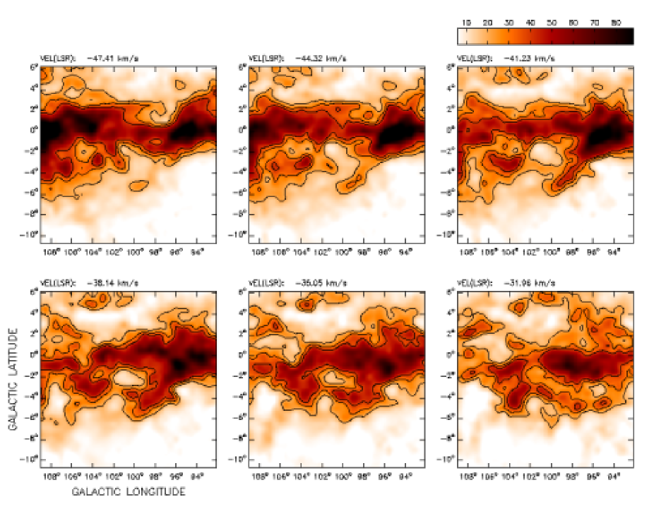
Figure 1: LAB H I  emission distribution averaged in the velocity range from $-47.41$ to $-31.96$ $\rm km\,s^{-1}$. Each image is an average of three velocity channel maps. Contour levels are at 20, 30, and 40 K. The LSR central velocity of each image is indicated in its top left corner. The color bar-code shows the temperature scale in kelvins for all the images.

Relying on the criteria described above, we are constructing a large H I  shells and supershells catalogue in the outer part of the Galaxy (Suad et al. in preparation). As part of this catalogue, we have found an H I  structure located at ($l,b$, $V$) = ($100\aas@@fstack{\circ}6$, $-2\aas@@fstack{\circ}3$, –41 $\rm km\,s^{-1}$). Following the standard nomenclature, this shell is labelled as GS 100–02–41 .

To illustrate the main observational findings, in Fig. 1 a mosaic of six H I  images covering the velocity range form $-47.41$ to $-31.96$ $\rm km\,s^{-1}$  is shown (all velocities in this paper are referred to the LSR). Each image is an average of three individual line channel maps and covers a velocity interval of about 3.09 $\rm km\,s^{-1}$.

The upper left panel shows the H I  brightness temperature distribution at $-47.41$ $\rm km\,s^{-1}$. Besides the H I  emission arising from the galactic plane, quite a few regions of low emissivity are clearly identified. These regions appear as a local minimum surrounded along most of its perimeter by regions of higher brightness temperature, as for example the structure located at ($l,b$) = (101$\aas@@fstack{\circ}$0, –2$\aas@@fstack{\circ}$0). As we move towards more positive velocities, this structure becomes a well defined H I  minimum within the overall galactic H I  emission. This minimum achieves its maximum angular extent at $-41.2$ $\rm km\,s^{-1}$  and is barely visible at $-32$ $\rm km\,s^{-1}$  (lower right panel).

An average of the H I emission distribution in the velocity range from $-42.26$ to $-34.02$ $\rm km\,s^{-1}$  is shown in Fig. 2, where a huge H I  structure having dimensions of $\sim\,6^{\circ}\times 3^{\circ}$ ($\Delta l$ $\times$ $\Delta b$) is easily recognizable.

To estimate the main parameters of this large H I  shell, we have characterized the ellipse that best fit it using a least square method. The points used to fit the ellipse correspond to the local maxima around the cavity. To select these points the CGPS H I  data were used. The parameters derived from this fit are: the symmetry centre of the ellipsoidal H I  distribution (l₀, b₀), the length of both the semi-major (a) and semi-minor (b) axes of the ellipse, and the inclination angle ($\theta$) between the major axis and the galactic longitude axis. This angle is positive towards the north galactic pole. They are given in Table 2.

Under the assumption of a symmetric expansion, an ellipsoidal H I  feature having a central velocity $V_{0}$ and an expansion velocity $V_{e}$ should depict, in a position-position diagram, an ellipse-like pattern when observed at different radial velocities. At $V_{0}$ the ellipse of H I  emission attains its maximum dimensions, while at extreme velocities (either approaching ($V_{\mathrm{m}}\,=\,V_{0}\,-\,V_{\mathrm{e}}$) or receding ($V_{\mathrm{M}}\,=\,V_{0}\,+\,V_{\mathrm{e}}$)) the hydrogen emission should look like an ”ovoidal” patch of emission. At intermediate velocities the dimension of the H I  ellipse shrinks as $V_{\mathrm{M}}\,$ (or $V_{\mathrm{m}}\,$) is approached. The expansion velocity is estimated as half of the total velocity range ($V_{e}=0.5\,(|V_{\mathrm{M}}\,-\,V_{\mathrm{m}}|)$) covered by the H I  emission related to the feature. This method always provides a lower limit to $V_{e}$, because H I  emission arising from those regions having radial velocities close to either the maximum approaching ($V_{\mathrm{m}}$) or receding ($V_{\mathrm{M}}$) cap are usually difficult to disentangle from the overall galactic H I  emission. Another way to determine $V_{\mathrm{e}}$ without the above drawback is to use the velocity-position diagrams. In Fig. 3 a radial velocity versus galactic longitude diagram is shown. This image shows a different view of GS 100–02–41 . The inner region of the elliptical H I  feature shown in Fig. 2, corresponds to the low emissivity region seen at ($V$, $l$) = ($-41$ $\rm km\,s^{-1}$, $100\aas@@fstack{\circ}6$). The strong peaks of H I  emission seen at $\sim-29$ $\rm km\,s^{-1}$  and $\sim-51$ $\rm km\,s^{-1}$  arise from the H I  associated with the expanding walls of neutral gas related to GS 100–02–41. Figure 4 shows a cross-cut of Fig. 3 along $l=100\aas@@fstack{\circ}6$. By making a Gaussian fit to the H I  emission peaks, $V_{\mathrm{m}}$ and $V_{\mathrm{M}}$ can be derived, along with the value of $V_{0}$, that corresponds to the velocity between $V_{\mathrm{m}}$ and $V_{\mathrm{M}}$ where the minimum value of $T_{b}$ is observed. We obtain $V_{0}$ = $-41\pm 2$ $\rm km\,s^{-1}$and $V_{\mathrm{e}}$ = $11\pm 2$ $\rm km\,s^{-1}$.

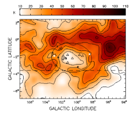
Figure 2: LAB H I  emission distribution averaged in the velocity range from –42.26 to –34.02 $\rm km\,s^{-1}$. Contour levels are from 10 to 90 in steps of 10 K. The area below the dashed line corresponds to the region where CGPS data are not available. The symbols indicate the location of the star members of Cep OB1 lying inside the ellipse (see Section 3.3). White star symbols correspond to O-type main sequence stars. Asterisks and triangles indicate evolved stars that were O-type and B-type stars during the main sequence phase, respectively.

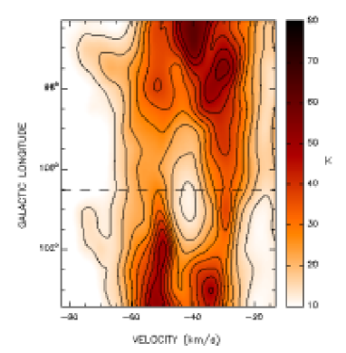
Figure 3: LAB H I  emission distribution averaged in the latitude range from –3$\aas@@fstack{\circ}$0 to –1$\aas@@fstack{\circ}$3. Contour levels are from 13 to 53 K in steps of 5 K. The dashed line indicates the location where the cross-cut shown in Fig. 4 was performed.

It is well known that non-circular motions on a large scale are present in the Perseus spiral arm (Brand & Blitz, 1993), making the galactic rotation model not suitable for this region of the Galaxy. Based on the observed velocity field derived by Brand & Blitz (1993), the systemic velocity of GS 100–02–41  can be translated to a kinematic distance of 2.8 $\pm$ 0.6 kpc. We shall adopt this distance for the H I  shell.

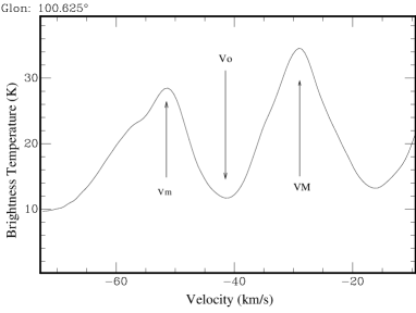
Figure 4: H I  cross-cut at l=100$\aas@@fstack{\circ}$6 obtained from Fig. 3 . The approaching ($V_{\mathrm{m}}$), systemic ($V_{0}$) and receding ($V_{\mathrm{M}}$) velocities are indicated.

Under the assumption that the H I  emission is optically thin and following the procedure described by Pineault (1998), the total neutral hydrogen mass of a structure located at a distance d (kpc) that subtends a solid angle $\Omega$ (square arc-min) is given by

$$M_{\mathrm{HI}}(M_{\odot})=1.3\times 10^{-3}\,\emph{d}^{2}\,\Delta V\,\Delta\emph{T}_{\mathrm{B}}\,\Omega$$

where $\Delta$V is the velocity interval over which the structure is detected, expressed in $\rm km\,s^{-1}$  and $\Delta T_{\mathrm{B}}$ (K) is the mean brightness temperature defined as $\Delta T_{\mathrm{B}}=\mid\emph{T}_{\mathrm{sh}}-\emph{T}_{\mathrm{bg}}\mid$, where T_sh refers to the mean brightness temperature of the H I  shell, and T_bg corresponds to the temperature of the contour level defining the outer border of the H I  shell. The latter represents the temperature of the surrounding galactic H I  emission gas. For this structure we estimated T${}_{\mathrm{sh}}=33.5\pm 1.6$ K, T${}_{\mathrm{bg}}=21.5\pm 1.5$ K, $\Delta$V $=22\pm 2$ $\rm km\,s^{-1}$and $\Omega=4.2\times 10^{4}$ arcmin². Adopting solar abundances, the total gaseous mass of GS 100–02–41  is $\emph{M}_{\mathrm{t}}(M_{\odot})=1.34\,M_{\mathrm{HI}}$ (see Table 2).

Assuming that the mass is uniformly distributed within the structure’s volume, we obtain the gas number density ($n_{sh}$) of the swept up gas. The ambient density ($n_{0}$) of the medium into which the large H I  shell is evolving is derived by uniformly distributing the shell mass ($M_{\mathrm{t}}$) over the volume swept up by the structure. Assuming this mass to be distributed into an ovoidal volume whose semi-major axis is a and the other two dimensions are set equal to b, then

$$n_{0}=10\frac{M_{\mathrm{t}}}{a\,b^{2}}\,\,(\mathrm{cm^{-3}})$$

where $M_{\mathrm{t}}$ is given in M_⊙, and a and b in parsecs.

A rough estimate of the age of the shell can be obtained using a simple model to describe the expansion of a shell created by a continuous injection of mechanical energy or by a supernova explosion. In this way, the dynamical age of GS 100–02–41  can be estimated as $t_{\rm dyn}=\alpha$ R / $V_{e}$ (Weaver et al., 1977), where R is the radius of the shell ($R=\sqrt{a\,b}$) , and $\alpha=0.25$ for a radiative supernova remnant (SNR) or $\alpha=0.6$ for a stellar wind shell.

Another important parameter that characterizes the shells is the kinetic energy, which is given by $\emph{E}_{\mathrm{k}}=0.5\,\emph{M}_{\mathrm{t}}\,V_{e}^{2}$. All the relevant parameters of GS 100–02–41  are given in Table 2.

Table 2: GS 100–02–41  main parameters.

Parameter	Value
Distance (kpc)	2.8 $\pm$ 0.6
($l_{0}$, $b_{0}$)	(100$\aas@@fstack{\circ}$6, –2$\aas@@fstack{\circ}$04)
a	2$\aas@@fstack{\circ}$56
b	1$\aas@@fstack{\circ}$69
$\theta$	–5$\aas@@fstack{\circ}$7
a (pc)	125$\pm$ 25
b (pc)	83 $\pm$ 17
$V_{0}$ ($\rm km\,s^{-1}$)	–41 $\pm$ 2
$V_{e}$ ($\rm km\,s^{-1}$)	11 $\pm$ 2
Mt (M⊙)	(1.5$\pm$ 0.7) $\times 10^{5}$
$n_{sh}$ (cm-3)	2.5 $\pm$ 0.4
$n_{0}$ (cm-3)	1.7 $\pm$ 0.4
$\emph{E}_{\mathrm{k}}$ (erg)	$(1.8\pm 0.8)\times 10^{50}$
tdyn ($\alpha=0.25$) (Myr)	2.3 $\pm$ 1.1
tdyn ($\alpha=0.6$) (Myr)	5.5 $\pm$ 2.7

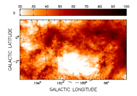
Figure 5: CGPS averaged H I  emission distribution in the velocity range from –42.7 to –34.4 $\rm km\,s^{-1}$. The dashed ellipse corresponds to the ellipse shown in Fig. 2.

Even though the CGPS data do not cover the whole area of GS 100–02–41, for completeness in Fig. 5 the CGPS data averaged in the same velocity range than the LAB data are shown. A comparison with Fig. 2 clearly shows that the large-scale structures are observed in both data sets and, as expected, a lot of small scale structures are observed in the high resolution image. The dashed ellipse shown in Fig. 5 is the one obtained form the fitting of the low resolution data (see Table 2).

3.2 Radio continuum and infrared data.

Figure 6 shows the observed radio continuum emission at 2695 MHz (upper panel) and the 60 $\mu$m infrared emission (lower panel) towards the region where GS 100–02–41  is detected.

No large scale features that could be interpreted as the counterpart of the H I  structure could be found neither in the radio continuum nor in the infrared images. The strong source observed at both frequencies at ($l,b$) $\simeq$ (102$\aas@@fstack{\circ}$8, –0$\aas@@fstack{\circ}$7) is the well known H II  region Sh2-132 , which has been recently studied by Vasquez et al. (2010). Towards the southwest of this H II  region, a ring nebula related to the Wolf-Rayet star WR 152 is also observed (Cappa et al., 2010). On the other hand, three slightly extended and much more weaker sources are seen projected onto the H I  shell. Following the standard nomenclature, they will be referred to as G103.39-2.28 (G103, for short), G100.7-0.5 (G100), and G98.51-1.7 (G98). These three sources will be analyzed in Section 4.

In the infrared image (see Fig. 6 lower panel) two sources, IRAS 22036+5306 (IR1) and IRAS 22142+5206 (IR2), located at ($l,b$) = ($99\aas@@fstack{\circ}63,-1\aas@@fstack{\circ}85$) and ($l,b$) = ($100\aas@@fstack{\circ}38,-3\aas@@fstack{\circ}58$), respectively, are observed. Neither of these sources has a counterpart at 2695 MHz. The first source is associated with a post AGB star, whilst the second one (IRAS 22142+5206) may be a protostellar object (Dobashi et al., 1998).

They found IRAS 22142+5206 to be associated with CO molecular emission at $V=-37.2$ $\rm km\,s^{-1}$.

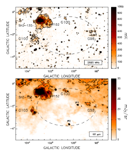
Figure 6: Upper panel. Effelsberg 2695 MHz emission distribution in the area of GS 100–02–41. Contour levels are at 65, 250 and 400 mK. Lower panel. IRIS 60 $\mu$n emission distribution. Contour levels are at 12, 18 and 24 mJy sr^-1. In both panels the ellipse marks the location of the large H I  shell.

3.3 large H I  shell origin.

The origin of GS 100–02–41  may be attributed to the action of the stellar wind of several massive stars and their subsequent supernova explosions. In the following, based on the derived parameters of the shell, we analyze both scenarios.

An inspection of the Galactic OB Associations in the Northern Milky Way Galaxy presented by Garmany & Stencel (1992) reveals that several stars belonging to Cep OB1 are seen projected inside the ellipse delineating GS 100–02–41. They are indicated by symbols in Fig. 2.

Garmany & Stencel (1992) determined for Cep OB1 a photometric distance modulus of DM = 12.2 mag, which yields a distance of 2.75 kpc. On the other hand, based on the stellar proper motions given by Hipparcos, Mel’Nik & Dambis (2009) estimated a distance of 2.8 kpc for this OB association. This distance is consistent with the distance estimate derived for GS 100–02–41  when non-circular motions are considered (Brand & Blitz, 1993). To test the possibility that the Cep OB1 stars lying inside the H I shell could have been capable of creating it, an evaluation of the energy that may be injected into the ISM by the early type stars of Cep OB1 is in place. Is the energy provided by these massive stars enough to create GS 100–02–41?

Those stars lying within the boundaries of GS 100–02–41, twenty in total, are listed in Table 3. Column 1 gives the star’s identification, Col. 2 and 3 their galactic coordinates, and Col.4 their spectral types as given by Garmany & Stencel (1992). Based on the evolutionary track models published by Schaller et al. (1992), and adopting the bolometric magnitudes and effective temperatures given by Garmany & Stencel (1992), we estimated the main sequence (MS) spectral type for each star (Col. 5). Column 6 gives an estimate of the star MS lifetime ($t$(MS)) as derived from the stellar models of Schaller et al. (1992). The values given in this column are a rough estimate as a consequence of the uncertainty in the mass adopted for each star. Column 7 and 8 give the mass loss rates ($\dot{M}$) and wind velocities ($V_{w}$) taken from Leitherer (1998), respectively. Column 9 gives the total wind energy released by each star during its main sequence phase, $E_{w}=0.5\,\dot{M}\,V_{w}^{2}\,t(\rm MS)$. Given that HDE 235673 and HDE 235825 are still in the MS, their values are upper limits.

Table 3: Cep OB1 stars lying inside GS 100–02–41.

Star	$l$	$b$	Sp. Type	MS Sp. Type	MS lifetime (Myr)	log ($\dot{M}$ (M${}_{\odot}yr^{-1}$))	$V_{w}$ ($\rm km\,s^{-1}$)	$E_{w}$($10^{50}$ erg)
HDE 235673	98$\aas@@fstack{\circ}$4	–1$\aas@@fstack{\circ}$6	O6.5 V	O6.5	5.6	–6.27	2700	$\leq$ 2.2
HD 209678	99$\aas@@fstack{\circ}$3	–1$\aas@@fstack{\circ}$8	B2 I	B0	12	–7.17	1600	0.2
HD 209900	99$\aas@@fstack{\circ}$7	–1$\aas@@fstack{\circ}$7	A0 Ib	B1	26	–8.2	2500	0.2
HD 210809	99$\aas@@fstack{\circ}$9	–3$\aas@@fstack{\circ}$1	O9 Iab	O7	6.4	–6.39	2700	2.1
BD +51 3135	100$\aas@@fstack{\circ}$6	–2$\aas@@fstack{\circ}$1	B3 II	B0.5	14	–7.3	1850	0.2
HDE 235781	101$\aas@@fstack{\circ}$2	–2$\aas@@fstack{\circ}$6	B6 Ib	B1	22	–8.2	2500	0.2
BD +53 2820	101$\aas@@fstack{\circ}$2	–1$\aas@@fstack{\circ}$7	B0 IV	B0	16	–7.17	1600	0.2
BD +52 2833	101$\aas@@fstack{\circ}$4	–2$\aas@@fstack{\circ}$1	B1 III	O9.5	10	–7.04	2500	0.5
BD +53 2837	101$\aas@@fstack{\circ}$5	–2$\aas@@fstack{\circ}$1	B2 III	B0.5	14	–7.3	1850	0.2
HDE 235783	101$\aas@@fstack{\circ}$7	–1$\aas@@fstack{\circ}$9	B1 Ib	B0.5	14	–7.3	1850	0.2
BD +53 2843	101$\aas@@fstack{\circ}$8	–2$\aas@@fstack{\circ}$2	O8 III	O7	6.4	–6.39	2700	2.1
BD +54 2718	102$\aas@@fstack{\circ}$0	–0$\aas@@fstack{\circ}$9	B2 III	B0.5	14	–7.3	1850	0.2
BD +54 2726	102$\aas@@fstack{\circ}$2	–1$\aas@@fstack{\circ}$0	B1.5 II	B0.5	14	–7.3	1850	0.2
HDE 235813	102$\aas@@fstack{\circ}$4	–2$\aas@@fstack{\circ}$0	B0 III	O6	6.3	–6.14	2700	2.6
HILTNER 1106	102$\aas@@fstack{\circ}$5	–0$\aas@@fstack{\circ}$7	B0 III	O8	6.9	–6.65	2600	0.9
BD +53 2885	102$\aas@@fstack{\circ}$7	–2$\aas@@fstack{\circ}$9	B2 III	B0.5	14	–7.3	1850	0.2
HD 212455	102$\aas@@fstack{\circ}$8	–1$\aas@@fstack{\circ}$7	B6 Ib	B0.5	14	–7.3	1850	0.2
HDE 235825	102$\aas@@fstack{\circ}$9	–1$\aas@@fstack{\circ}$8	O9 V	O9	8	–6.91	2500	$\leq$0.6
BD +54 2764	103$\aas@@fstack{\circ}$0	–1$\aas@@fstack{\circ}$7	B1 Ib	B0.5	14	–7.3	1850	0.2
BD +54 2761	103$\aas@@fstack{\circ}$1	–1$\aas@@fstack{\circ}$4	O6 III	O3*	4.3	–5.43	3200	$\leq$16.3

*: The bolometric magnitude and effective temperature given by Garmany & Stencel (1992) lie outside the evolutionary tracks of Schaller et al. (1992). We adopted for this star the earliest spectral type.

Theoretical models predict that only 20 % of the wind energy is converted into mechanical energy of the shell (Weaver et al., 1977). In the case of GS 100–02–41 , this implies that for the total kinetic energy stored in the shell, $E_{k}=(1.8\pm 0.8)\times 10^{50}$ erg, a wind energy greater than 9 $\times 10^{50}$ erg would be required. However the analysis of several observed H I  shells shows that the energy conversion efficiency seems to be lower, roughly about 2-5 % (Cappa et al., 2003).

From the last column of Table 3 we infer that the total wind energy injected during the MS phase of the Cep OB1 stars is $\sim 29.7\times 10^{50}$ erg, which is enough to create GS 100–02–41  if the energy conversion efficiency were $\sim$ 6 %.

It is important to mention that the MS lifetime of all the O stars, which are the main energy contributors, is compatible, within errors, with the dynamical age of the shell (5.5 $\pm\,2.7$ Myr). Moreover, the fact that most of the massive stars located inside the shell are evolved stars may explain the absence of ionized gas related to GS 100–02–41.

On the other hand, taking into account that the SN rate in a typical OB association is about one per $10^{5}-3\times 10^{5}$ yr. (McCray & Kafatos, 1987), over the lifetime of GS 100–02–41  is reasonable to assume that the most massive members of Cep OB1 may have exploded as SN. In this case, the energy of the explosions, as well as the energy injected by the stellar winds of the SNe progenitors, would have also contributed to the formation of the shell. There is no detection of a SNR in either radio surveys or x-ray surveys, but this could be due to the relatively large age of GS 100–02–41. However, an evidence that a SN explosion could have taken place in the region is the presence of the pulsar PSR J2150+5247, located at ($l,b$) = (97$\aas@@fstack{\circ}$5, –0$\aas@@fstack{\circ}$9) (Taylor et al., 1993). Even though the estimated distance to the pulsar is 5.48 kpc (Taylor et al., 1993), bearing in mind that this distance is obtained based on the dispersion measure and a galactic electron density model (Taylor & Cordes, 1993), the error is large, and therefore the possibility that the pulsar were located at a distance similar to the one of GS 100–02–41  can not be ruled out. Were this the case, an upper age limit for the progenitor of PSR J2150+5247, assuming it was an early B-type star, would be $\sim$3 $\times$ 10⁷ yr, that is in reasonable agreement with the age of the oldest star, HD 209900, belonging to Cep OB1.

4 Sources G98, G100, and G103

4.1 Their Nature.

As mentioned in Section 3.2, three slightly extended sources, labelled G98, G100, and G103, are observed at radio continuum and infrared wavelengths, projected onto the border of GS 100–02–41. The upper panels of Fig. 7 show the CGPS 1420 MHz radio continuum image of each source. In these images, discrete sources have been removed. The middle panels show the HIRES 60 $\mu$m emission distribution in the area of G98, G100, and G103. At both fequencies, to increase the signal-to-noise ratio, the original images were smoothed to a 2-arcmin resolution.

A clue onto their physical nature (thermal or non-thermal) may be provided by the behavior of the flux density as a function of frequency. Previous flux density estimations for G100 were obtained by White & Becker (1992) and Kerton et al. (2007). White & Becker (1992) obtained a flux density at 1420 MHz of 456 mJy, while Kerton et al. (2007) estimated a lower flux density, S${}_{1420}=48.8\pm 24.0$ mJy. To estimate the spectral index $\alpha$ ($S_{\nu}\propto\nu^{-\alpha}$) of each source, CGPS continuum observations at 408 and 1420 MHz, and Effelsberg continuum data at 2695 MHz were used in this work.

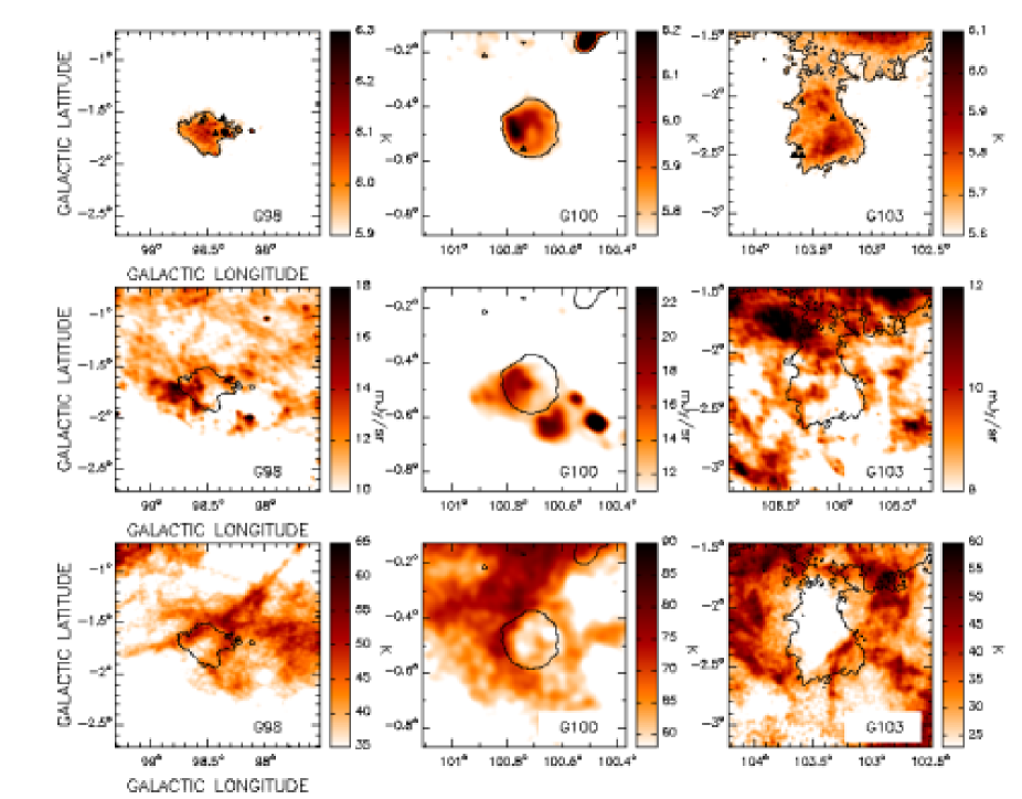
Figure 7: Upper panels 1420 MHz radio continuum images in the area of G98 (left), G100 (middle), and G103 (right). Point-like sources have been removed. Contour levels are at 6.0, 5.8, and 5.6 K, for G98, G100, and G103, respectively. The black triangle symbols indicate the location of the stars HD 235673, ALS 12073, ALS 12071 and ALS 12074 (G98), BD+542684 (G100), and ALS 12434, ALS 12443, ALS 12471, ALS 12469 and ALS 12475 (G103). Middle panels: HIRES 60 $\mu$m emission distribution in the area of G98, G100 and G103. For comparison with the 1420 MHz emission, contour levels are the same as in upper panels. Lower panels: CGPS H I  emission distribution averaged in the velocity range from –41.9 to – 50.9 $\rm km\,s^{-1}$  in the area of G98 (left), from –50.9 to –55.9 $\rm km\,s^{-1}$  in the area of G100 (middle) and from –29.5 to –31.15 $\rm km\,s^{-1}$  in the area of G103 (right). Contour levels are the same as for upper and middle panels. In all images the angular resolution is 2-arcmin.

Flux density determinations, specially for weak sources like the ones we are dealing with, are strongly dependent on the source angular extent, which in turns depends on the outermost reliable continuum level. Before defining the angular extent of each source, the overall galactic continuum emission has to be subtracted out. To this end we applied the ”Back Ground Filtering” method (BGF) developed by Sofue & Reich (1979). A 1$\degr\times$1$\degr$ filtering beam was applied to all sources at each frequency.

The derived flux densities are given in Table 4. The quoted errors stem from the uncertainty in determining the background levels. The spectral index $\alpha$ was derived from a fit to the observed flux densities, under the assumption that none of these sources is optically thick at the lowest frequency (408 MHz). For G100 a residual grating ring from the strong nearby Cas A source falls on top of the source, making the estimate of the 408 MHz flux density meaningless. The lower flux density obtained by Kerton et al. (2007) is consistent with the smaller area considered for G100 by these authors. On the other hand, the higher value given by White & Becker (1992) may be attributed to the fact that they used Green Bank data (HPBW $\sim 11\arcmin$).

Though highly uncertain, the spectral indexes are consistent with a thermal nature for G98, G100, and G103; implying that they are H II  regions. Another argument in favor of this interpretation comes from the far infrared data. From the measured flux densities at 60 and 100 $\mu$m and following the procedure descibed by Cichowolski et al. (2001), the dust temperature was estimated for each region (see Table 4). The derived temperatures are typical of H II  regions. The errors quoted for the dust temperatures are formal errors from the fitting procedure.

Table 4: G98, G100 and G103 parameters.

Source	G98	G100	G103
Longitude	98$\aas@@fstack{\circ}$5	100$\aas@@fstack{\circ}$7	103$\aas@@fstack{\circ}$3
Latitude	–1$\aas@@fstack{\circ}$6	–0$\aas@@fstack{\circ}$5	–2$\aas@@fstack{\circ}$4
Size (arcmin)	73 x 64	19 x 23	54 x 87
S408 (Jy)	2.1 $\pm$ 0.3	–	2.0 $\pm$ 0.3
S1420 (Jy)	2.0 $\pm$ 0.1	0.21 $\pm$ 0.03	1.50 $\pm$ 0.15
S2695 (Jy)	1.9 $\pm$ 0.3	0.19 $\pm$ 0.03	1.70 $\pm$ 0.35
Spectral index $\alpha$	–0.05 $\pm$ 0.01	–0.16 $\pm$ 0.33	–0.11 $\pm$ 0.08
S60 (Jy)	410 $\pm$ 20	120 $\pm$ 6	1030 $\pm$ 50
S100 (Jy)	1640 $\pm$ 80	380 $\pm$ 20	1840 $\pm$ 90
Dust temperature (K)	24.5 $\pm$ 0.7	26.5 $\pm$ 0.8	33.1 $\pm$ 1.1

4.2 Location of G98, G100 and G103.

We now try to discern whether these ionized regions could be physically related to GS 100–02–41. Unfortunately, the radio continuum flux densities of G98, G100 and G103 are not strong enough to allow us to derive a reasonable H I  absorption spectrum in order to attempt to set a limit to their distances. Another way to attempt to estimate their distances is to look for signatures of the interaction among the ionized regions and the H I  and CO gas emission observed around these sources. If the continuum sources were related to GS 100–02–41, the H II  regions would expand within the gas of GS 100–02–41  and we would be able to observe for each source an H I  minimum in a velocity range compatible with the radial velocity of the large H I  shell. After a thorough inspection of the CGPS H I  data cube, we were able to point down H I  minima having a good morphological correlation with the radio continuum sources.

Mean brightness temperature of these structures are shown in the lower panels of Fig. 7 (the original images were smoothed to a 2-arcmin resolution). The radial velocity ranges where these minima are detected range from –40.2 to –51.8 $\rm km\,s^{-1}$  (G98), from –50.1 to –58.4 $\rm km\,s^{-1}$  (G100), and from –22.1 to –33.6 $\rm km\,s^{-1}$  (G103). However, it is important to mention that for the averages shown in Fig. 7 only those velocity channels where the minima are best defined were considered. To facilitate the comparison among the radio continuum and the H I  emission distributions, the 1420 MHz contour line defining the source’s extent is superimposed on the H I images.

The H II  regions are clearly surrounded by enhanced H I  emission. The positional coincidence between the H I  features and their corresponding H II  region suggests that they are physically related. It is worth mentioning that, although the entire velocity cube was searched for H I  features likely to be related to the ionized regions, no other peculiar structures but the ones shown in Fig. 7 were found.

We have also analyzed the CO emission distribution in the area of G100 and G103 (unfortunately there is no CO data available for G98). We found two molecular clouds probably related to G100 in the velocity range form $-52.25$ to $-55.17$ $\rm km\,s^{-1}$  (black contours in Fig. 8), in coincidence with the velocity range where the H I  structure was found. Figure 8 also shows the MSX Band A (8.28 $\mu$m) image (red colours) and the 5.8 K level at 1420 MHz (blue contour). Clearly, the 8.28 $\mu$m emission partially borders the ionized gas. It is worth mentioning that the emission observed in the MSX Band A is not detected in the other three MSX bands (12.13 $\mu$m, 14.65 $\mu$m, and 21.3 $\mu$m), suggesting that the polycyclic aromatic hydrocarbons (PAHs) could be the main responsible for the emission detected at 8.28 $\mu$m, indicating the presence of a photo-dissociated region (PDR) in the border of G100. An inspection of the CO data cube in the area of G103 do not reveal any CO structure probably related to the H II  region.

Bearing in mind that GS 100–02–41  is detected in the velocity range from $-29$ to $-51.7$ $\rm km\,s^{-1}$  and that its baricentral velocity is $V_{0}=-41\pm 2$ $\rm km\,s^{-1}$, we would locate both G98 and G100 in the approaching hemisphere of GS 100–02–41, whilst G103 would be placed in its receding part. In what fallows we adopt for the H II  regions the GS 100–02–41  distance.

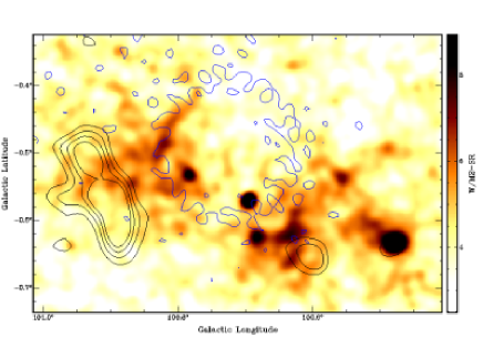
Figure 8: 8.3 $\mu$m emission distribution in the area of G100. The blue contour correspond to the 5.8 K level at 1420 MHz. Black contours are associated with the CO emission distribution averaged between –52.25 and –55.17 $\rm km\,s^{-1}$, at 0.4, 0.6, 0.8 and 1.0 K.

4.3 Exciting stars of G98, G100, and G103.

To identify the exciting stars of G98, G100, and G103 we have inspected the Galactic O Star Catalogue (Sota et al., 2008) and the OB Star Catalogue (Reed, 2003) looking for massive stars located in projection toward the H II regions.

Only one star projected within the border of G98 is listed by Sota et al. (2008), whilst in the Reed catalogue four stars are seen projected towards G98 (one of them coincides with the one catalogued by Sota et al. (2008)), one onto G100 , and five onto G103. They are listed in Table 5 and their positions are indicated by triangle symbols in Fig.7. It is worth mentioning that HD 235673, the star seen projected onto G98, appears in Table 3 as a Cep OB1 member and therefore was considered as an input energy source for the creation of GS 100–02–41. Nonetheless its contribution to the overall energy budget is $\sim$ 7 %, so if this star were related to G98, its exclusion as being responsible in the creation of GS 100–02–41  would not modify the conclusions reached in Section 3.3.

To check whether these stars may have contributed to the creation of the observed structures, under the assumption that they are located at the same distance than the H II  regions (2.8 $\pm$ 0.6 kpc), we analyze if their absolute magnitudes are compatible with those corresponding to OB-type stars. We need first to estimate the visual absorption in the region. From an averaged H I  profile (from 0 to –41 $\rm km\,s^{-1}$) of all over the solid angle covered by GS 100–02–41, we derive a total H I  column density of about $N_{{H\textsc{I}}}=3\times 10^{21}$ cm^-2. Using the relation $A_{v}=5.3\times 10^{-22}N_{{H\textsc{I}}}$ (Bohlin et al., 1978), we estimate $A_{v}=1.6$ mag. As a check on this, for HD 235673 we estimated the visual absorption using $A_{v}=3.1\,E(B-V)$, where $E(B-V)=(B-V)-(B-V)_{0}$. For $(B-V)_{0}=-0.32$ (Schmidt-Kaler, 1982) and $(B-V)=0.21$ (Hiltner & Johnson, 1956) we obtain $A_{v}=1.6$. Both values are in agreement with the absorption of 1-2 mag given by Neckel & Klare (1980).Then, adopting a visual absorption of 1.6 mag, the absolute magnitudes (see Column 5) of the stars listed in Table 5 were calculated. Based on Martins & Plez (2006) and Schmidt-Kaler (1982), the corresponding spectral types were estimated (see Col. 6 of Table 5).

Given that at the assumed distance all the stars listed in Table 5 could be O- or early B-type stars, we suggest that they may be responsible of creating G98, G100, and G103.

Table 5: OB stars probably related to G98, G100, and G103.

Star	Galactic coordinates ($l,b$)	Sp. Type	v (mag)	M${}_{v}^{(a)}$	Sp. Type(a)
G98
HD 235673(b)	98$\aas@@fstack{\circ}$36, –1$\aas@@fstack{\circ}$55	O7	9.14	–4.7 $\pm$ 0.5	O5/O8.5
ALS 12073	98$\aas@@fstack{\circ}$43, –1$\aas@@fstack{\circ}$71	OB	12.1	–1.7 $\pm$ 0.5	B2/B5
ALS 12071	98$\aas@@fstack{\circ}$53, –1$\aas@@fstack{\circ}$55	OB	12.25	–1.6 $\pm$ 0.5	B2/B5
ALS 12074	98$\aas@@fstack{\circ}$55, –1$\aas@@fstack{\circ}$59	OB	12.04	–1.8 $\pm$ 0.5	B2/B5
G100
BD +542684	100$\aas@@fstack{\circ}$74, –0$\aas@@fstack{\circ}$55	OB	10.8	–3.0 $\pm$ 0.5	B0/B2
G103
ALS 12434	103$\aas@@fstack{\circ}$32, –2$\aas@@fstack{\circ}$18	B5	10.6	–3.2 $\pm$ 0.5	B0/B2
ALS 12443	103$\aas@@fstack{\circ}$59, –2$\aas@@fstack{\circ}$04	OB	12.6	–1.2 $\pm$ 0.5	B3/B7
ALS 12471	103$\aas@@fstack{\circ}$59, –2$\aas@@fstack{\circ}$50	OB	12.4	–1.4 $\pm$ 0.5	B2/B7
ALS 12469	103$\aas@@fstack{\circ}$61, –2$\aas@@fstack{\circ}$44	B2	10.6	–3.3 $\pm$ 0.5	B0/B2
ALS 12475	103$\aas@@fstack{\circ}$66, –2$\aas@@fstack{\circ}$50	B2	11.4	–2.4 $\pm$ 0.5	B1/B3

(a): For the adopted distance of 2.8 $\pm$ 0.6 kpc. (b): Star found in both catalogues and member of Cep OB1 (Garmany & Stencel, 1992).

Next, we should consider whether the number of UV ionizing photons needed to keep the continuum sources ionized could be provided by their probably exciting stars. The total number of Lyman continuum photons is given by N${}_{Lym}=0.76\times 10^{47}\,$T${}_{4}^{-0.45}\,\nu_{\rm GHz}^{0.1}$D${}_{\rm kpc}^{2}$  S_ν (Chaisson, 1976), where T₄ is the electron temperature in units of $10^{4}$ K, D_kpc is the distance in kpc, $\nu_{\rm GHz}$ is the frequency in GHz and S_ν is the measure flux density in Jy. Using the 1420 MHz flux densities given in Table 4, a distance of 2.8 kpc and adopting T₄ = 1, we obtained N${}_{Lym}=1.2\times 10^{48}$ s^-1 for G98, N${}_{Lym}=1.3\times 10^{47}$ s^-1 for G100, and N${}_{Lym}=1.8\times 10^{48}$ s^-1 for G103. According to the theoretical models of Schaerer & de Koter (1997), for solar metallicity, the estimated N_Lym necessary to keep G98, G100, and G103 ionized, could be provided by a O9.5V, B0.5V, and O9.5V stars (or two B0V), respectively. This indicates that the join action of the stars listed in Table 5 can provide the ionizing photons needed for each H II region. In the case of G98, given that the contribution of HD 235673 is essential to keep this region ionized, we conclude that this star is associated with G98 instead of being related to the genesis of GS 100–02–41  as it was considered in Section 3.3. This implies that the wind energy provided for this star should not have been taken into account for the origin of GS 100–02–41. As mentioned before, this fact does not affect the scenario proposed for the creation of the large H I  shell.

5 Triggered star formation?

It is generally believed that expanding shells may induce star formation at their edges (Elmegreen, 1998). Shells behind shock fronts experience gravitational instabilities that may lead to the formation of large condensation inside the swept-up gas, and some of them may produce new stars. An increasing body of observational evidence supports the importance of the shell’s evolution in creating new stars (Patel et al., 1998; Oey et al., 2005; Arnal & Corti, 2007; Cichowolski et al., 2009; Cichowolski & Pineault, 2011).

In our case, having an old large H I  shell containing several H II  regions in its edge that seems to be at the same distance, we wonder if this could be other case of triggered star formation. Were this the case, we should expect an age gradient in the region, in the sense that G98, G100, and G103 should be younger than GS 100–02–41. In what follows we shall attempt to estimate the age of the H II  regions G98, G100, and G103, and compare them with the dynamical age of GS 100–02–41  estimated in Section 3.1 (see Table 2).

As a rough estimate to the age of each region, we evaluate their dynamical ages as $t_{dyn}=0.6\,R/V_{e}$ (Weaver et al., 1977). The radius $R$ of each region was estimated from the sizes given in Table 4. We infer $R=27.8\,\pm\,6.0$, $8.5\,\pm\,1.8$ and $27.9\,\pm\,6.0$ pc, for G98, G100 and G103, respectively, where the errors stem from the uncertainty in the distance. Relying on the velocity ranges were the H I  emission associated with each H II  region is observed (see Section 4), expansion velocities of 5.8 $\rm km\,s^{-1}$  (G98), 4.2 $\rm km\,s^{-1}$  (G100) and 5.8 $\rm km\,s^{-1}$  (G103) are assumed. Thus, we obtain an age of 2.9 $\pm\,0.9$, 1.2 $\pm\,0.5$ and 2.9 $\pm\,0.9$ Myr for G98, G100, and G103, respectively. The quoted errors stem from the uncertainties in the sizes and from the assumption that the expansion velocities are accurate to within 1.3 $\rm km\,s^{-1}$  (one velocity channel).

From these estimates, we conclude that G98, G100, and G103 are younger than GS 100–02–41. This age difference is supported by the fact that most of the stars probably responsible of creating GS 100–02–41  have already evolved from the MS, while the ionized gas of the H II  regions is still observed.

As mentioned in Section 3.2, in addition to G98, G100, and G103, three interesting sources are seen projected onto the border of GS 100–02–41: the H II  region Sh2-132, the ring nebula associated with WR 152, and the infrared source IRAS 22142+5206.

Regarding Sh2-132 and the ring nebula associated with WR 152, Vasquez et al. (2010) and Cappa et al. (2010) found neutral gas interacting with the H II regions in the velocity ranges from –38 to –53 $\rm km\,s^{-1}$  and from –43 to –52 $\rm km\,s^{-1}$ , respectively. For Sh2-132 this is in coincidence with the ionized velocity gas (Georgelin & Georgelin, 1976; Chu & Treffers, 1981; Reynolds, 1988; Fich et al., 1990; Quireza et al., 2006). Taking into account non-circular motions in this part of the Galaxy (Brand & Blitz, 1993), Vasquez et al. (2010) and Cappa et al. (2010) inferred for these regions a kinematical distance of $3.5\pm 1.0$ kpc. They argued that this value is in close agreement with the distance estimates of the main exiting stars of the regions, WR 153ab and WR 152. On the other hand, bearing in mind that GS 100–02–41 is observed in the velocity range from –29.0 to –51.7 $\rm km\,s^{-1}$ , and that the H II  regions are located onto its border, we suggest that both ionized structures may be located at the same distance as GS 100–02–41, and that the velocity differences are because the H II  regions are located in the approaching part of the large shell. Although Vasquez et al. (2010) do not give any age estimate for Sh2-132, the fact that it is being ionized by WR 153ab, implies that Sh2-132 should be older than the period of time spent by the progenitor of the WR in the main sequence phase. Given that WR 153ab is a WN6.5 star, the mass of the progenitor was probably about 40-50 $M_{\odot}$ (Crowther, 2007). According to Schaller et al. (1992) the MS lifetime for such a star is about 4 Myr. Concerning the age of the ring nebula associated with WR 152, Cappa et al. (2010) estimated a dynamical age of 1 Myr for the associated wind blown bubble. However, knowing that, as mentioned by Cappa et al. (2010), large errors are involved in this estimate and bearing in mind the time that the progenitor of the WR star spent in the MS phase, the age of the H II  region is probably higher, closer to the one estimated above for Sh2-132.

With respect to IRAS 22142+5206, as mentioned in Section 3.2, this infrared source has a massive molecular outflow associated with it at the velocity of –37.2 $\rm km\,s^{-1}$  (Dobashi et al., 1998). The coincidence between this velocity and the velocity range where GS 100–02–41  is observed suggests they may be located at the same distance. Based on the total luminosity of IRAS 22142+5206, Dobashi et al. (1998) suggest that this source will evolve into a late O-type or an early B-type star.

In summary, the fact that G98, G100, G103, Sh2-132, the ring nebula associated with WR 152, and IRAS 22142+5206 lie at the edge of GS 100–02–41  and seems to be at the same distance, together with the age gradient, suggest that these sources could have been triggered by the expansion of GS 100–02–41.

6 Conclusions

The large H I  shell GS 100–02–41  has been analyzed to study the interaction of massive stars with the interstellar medium and, in particular, the process of triggered star formation. From this analysis we conclude the following:

1. GS 100–02–41  is a large shell of a radius of about 102 pc located at a distance of 2.8 $\pm\,$ 0.6 kpc. The swept up mass in the shell is ($1.5\pm\,0.7$) $\times\,10^{5}$ M_⊙ and the shell density $n_{sh}=2.5\pm\,0.4$ cm^-3. The shell is expanding at a velocity of 11 $\pm\,2$ $\rm km\,s^{-1}$  and its kinetic energy is ($1.8\pm\,0.8$) $\times\,10^{50}$ erg.

2. Several evolved massive stars members of Cep OB1 are projected inside the large shell. The distance to the OB association is compatible with the kinematical distance of GS 100–02–41  when non-circular motions are considered. An energetic analysis suggests that the wind energy provided during the main sequence phase of the stars could explain the origin of the shell. However, taking into account the SN rate in OB associations, the energy contribution of a SN explosion as well as of its massive progenitor can not be discarded.

3. From the 2695 MHz radio continuum and 60 $\mu$m infrared images, we found three slightly extended sources, labelled G98, G100, and G103 projected onto the borders of GS 100–02–41. From the radio flux densities estimated at different wavelengths, the thermal nature of the sources was confirmed by the estimation of their spectral indexes. In addition, dust temperatures were estimated and found to be typical of H II  regions.

4. An inspection of the 1^′  CGPS H I  data reveals H I  minima having a good morphological correlation with the H II  regions at velocity ranges compatible with the velocity spanning by GS 100–02–41. This leads to the conclusion that G98, G100, and G103 are located at the same distance than GS 100–02–41.

5. From O and OB star catalogues, the massive star candidates to be responsible for the ionized gas were identified.

6. The obtained age difference among the H II  regions and the shell, together with their relative location leads us to the conclusion that G98, G100, and G103 may have been created as a consequence of the action of a strong shock produced by the expansion of GS 100–02–41  into the surrounding gas.