I Introduction

AdS/CFT is a powerful tool Maldacena:1997re ; Witten:1998qj ; Gubser:1998bc which among other things allows us to compute CFT correlators at strong coupling via Witten diagrams in AdS space. In practice these computations are still quite challenging in position space and generally require a lot of work, see LiuTseytlin ; hep-th/9811152 ; D'Hoker:1998mz ; Freedman:1998bj ; Freedman:1998tz ; D'Hoker ; Arutyunov:2000py ; Arutyunov:2002fh ; Arutyunov:2003ae ; Berdichevsky:2007xd ; Uruchurtu:2008kp ; Buchbinder:2010vw ; Uruchurtu:2011wh ; Dolan:2006ec ; Howtozintegrals ; Raju1 ; Raju2 . Recently it has been argued that taking the Mellin transform of correlation functions drastically simplifies the computations and the resulting expressions have nice mathematical structure, see e.g. Mack:2009mi ; Mack:2009gy ; Penedones:2010ue ; Paulos:2011ie ; Fitzpatrick:2011ia ; Costa:2011mg ; Costa:2011dw ; arXiv:1102.0577 . The correlation functions of primary scalar operators for a CFT can be written in Mellin space as

$$\langle\mathcal{O}(x_{1})\mathcal{O}(x_{2})\ldots\mathcal{O}(x_{n})\rangle\sim\int\mathrm{d}\delta_{ij}M(\delta_{ij})\!\prod_{1\leq i<j\leq n}\!\!\Gamma(\delta_{ij})\,(x^{2}_{ij})^{-\delta_{ij}},$$ (1)

where $M(\delta_{ij})$ is called the Mellin amplitude and parameters $\delta_{ij}$ can be parametrized as $\delta_{ij}=k_{i}\cdot k_{j}$. Mellin amplitudes have many similarities to scattering amplitudes in flat space, in particular the large AdS radius limit of the Mellin amplitude was argued to be equivalent to the scattering amplitudes in flat space Penedones:2010ue ; Fitzpatrick:2011ia , such that $k_{i}$ plays the role of momentum in flat space, suggesting that Mellin amplitudes could be used to provide a holographic definition of the S-matrix, see susskind ; polchinski ; GGP ; JP ; Katz ; TakuyaFSL ; Fitzpatrick:2011jn ; Gary:2009mi ; GiddingsBulkLoc ; Gary:2011kk for related discussion.

More recently in Paulos:2011ie and Fitzpatrick:2011ia , the authors studied various aspects of the Mellin representation of AdS correlators. In particular, a set of Feynman rules, for computing Mellin amplitudes for any theory of scalar field at tree-level, was proposed and checked for a few non-trivial correlators in $\phi^{3}$ and $\phi^{4}$ theories in Paulos:2011ie as well as recursively via a factorization formula for $\phi^{3}$ theory in Fitzpatrick:2011ia .

In this note we will consider a scalar field with $\phi^{n}$ interaction at tree level and offer a direct proof of the Feynman rules for Mellin amplitudes by evaluating all the Witten diagram integrals explicitly. We hope that our results will be useful for better understanding of the structure of Mellin amplitudes and for the future development of similar rules for fields with spin and for loop amplitudes. We have also checked that the Mellin space Feynman rules reduce to the usual Feynman rules in the flat space limit.

The paper is organized as follows. In section $2$ we review the conjectured Feynman rules for Mellin amplitudes. In section $3$ we use particular forms of the bulk-to-boundary and bulk-to-bulk propagators to compute the Witten diagram with the maximal off-shell vertex for a $\phi^{n}$ theory and show that they lead to the conjectured Feynman rules for Mellin amplitudes. Then we demonstrate that we get the same Feynman rules for such a vertex embedded in a very general Witten diagram of the $\phi^{n}$ theory. In section $4$ we show that these Feynman rules reduce to the usual Feynman rules in the flat space limit.

Note added: While this paper was in preparation, the paper Fitzpatricknew appeared which checks the formula for the off-shell $n$-pt vertex of the $\phi^{n}$ theory via recursion relations.

II Feynman rules for Mellin amplitudes

Let us first review the Feynman rules for Mellin amplitudes corresponding to any tree level Witten diagram in AdS_d+1 for a $\phi^{n}$ scalar theory, as proposed in Paulos:2011ie . To compute the Mellin amplitude one has to put together propagators and vertices following a few simple steps:

$-$ Assign a “momentum” $k_{i}$ to every line such that the external lines of the Witten diagram have $-k_{i}^{2}=\Delta_{i}$ and at each vertex we have conservation $\sum_{i}k_{i}=0$, where $\Delta_{i}$ is the conformal dimension of the corresponding field.

$-$ Assign an integer $m_{i}$ to each internal line with the propagator

$${\cal P}_{i}=\frac{-1}{2m_{i}!\Gamma(1+\Delta_{m_{i}}+m_{i}-h)}\ \frac{1}{k_{i}^{2}+(\Delta_{m_{i}}+2m_{i})},$$ (2)

where $h=d/2.$

$-$ The factor for a vertex connecting lines with dimension $\Delta_{i}$ and integers $m_{i}$, (see Fig. 1) is given by

$$V^{\Delta_{1}\ldots\Delta_{n}}_{[m_{1},\ldots,m_{n}]}=g^{(n)}\,\Gamma\left(\frac{\sum_{i=1}^{n}\Delta_{i}-2h}{2}\right)\left(\prod_{i=1}^{n}\left(1-h+\Delta_{i}\right)_{m_{i}}\right)$$

$$F_{A}^{(n)}\left(\frac{\sum_{i=1}^{n}\Delta_{i}-\!2h}{2},\left\{-\!m_{1},\ldots,-\!m_{n}\right\},\left\{1\!+\!\Delta_{1}\!-\!h,\ldots,1\!+\!\Delta_{n}\!-\!h\right\};1,\ldots,1\right)\hskip 28.45274pt\ \ \$$ (3)

where $g^{(n)}$ is the coupling in the $g^{(n)}\phi^{n}$ theory, $(a)_{m}={\Gamma(a+m)\over\Gamma(a)}$ is the Pochhammer symbol and $F_{A}^{(n)}$ is the Lauricella function of $n$ variables

$$F_{A}^{(n)}\left(y,\left\{a_{1},\ldots,a_{n}\right\},\left\{b_{1},\ldots,b_{n}\right\};x_{1},\ldots,x_{n}\right) = \sum_{l_{i}=0}^{\infty}\left((y)_{\sum_{i=1}^{n}l_{i}}\prod_{i=1}^{n}\frac{(a_{i})_{l_{i}}}{(b_{i})_{l_{i}}}\frac{x_{i}^{l_{i}}}{l_{i}!}\right).$$ (4)

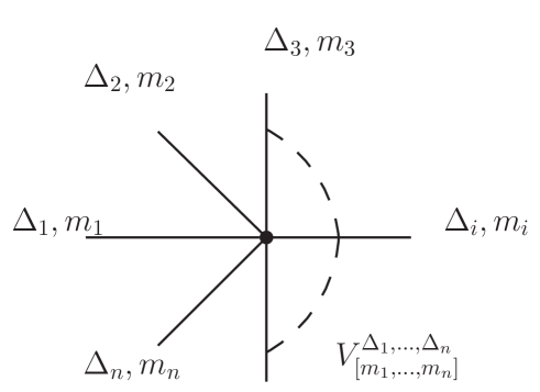
Figure 1: A general vertex for $\phi^{n}$ theory.

$-$ Finally, sum over all positive integers $m_{i}$ to obtain the Mellin amplitude.

We note here that the vertex given above is the most general type of vertex (or the maximal off-shell vertex) when all legs are off-shell, but the theory would also have vertices with less number of off-shell legs. The vertex factor in such cases can be simply obtained from the general case by taking some of the $m_{i}$’s to zero, corresponding to the legs going on-shell. Also, note that the Lauricella function of $m$ variables can be written in a series form as in (4) which is convergent for $\sum_{i}|x_{i}|<1$. For the vertex above, all $n$ variables $x_{i}$ take a particular value $1$, which is the Lauricella function evaluated at that particular point, which is well-defined via analytic continuation.

III Proof of Feynman rules

III.1 Maximal off-shell vertex

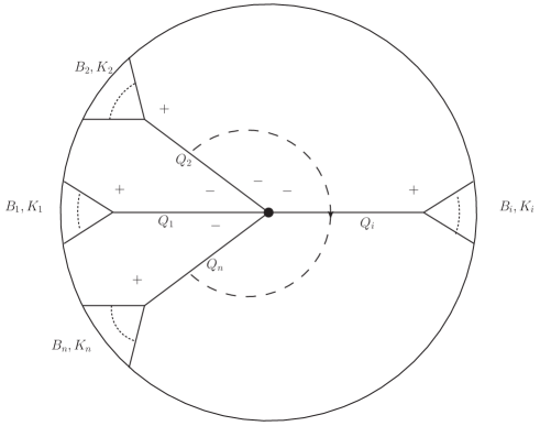
Figure 2: The Witten diagram for the scalar $\phi^{n}$ theory with a vertex having $n$ off-shell legs and $n$ vertices having $1$ off-shell leg and $(n\!-\!1)$ on-shell legs.

In this section we consider a Witten diagram for the scalar $\phi^{n}$ theory in AdS_d+1 which has a vertex with the maximal number of off-shell legs (see Fig. 2) and prove the Feynman rules for this case which we described in the previous section.

Let $X^{I}$ be the coordinates of the Euclidean AdS_d+1 space, embedded in a $d+2$ dimensional Minkowski space such that $X^{2}=-R^{2},$ where $R$ is the AdS radius and the point on the boundary $P^{A}$ defined on the light-cone such that $P^{2}=0$. The bulk-to-boundary propagator between a point $P$ on the boundary and $X$ in the bulk for a scalar field of dimension $\Delta$ is given by

$$E(P,X)=\frac{1}{2\pi^{h}\Gamma(1+\Delta-h)}\int_{0}^{+\infty}\frac{\mathrm{d}t}{t}t^{\Delta}\,e^{2tP\cdot X}.$$ (5)

The bulk-to-bulk propagator between the points $X_{1}$ and $X_{2}$ can be written as an integral over a point $Q$ on the boundary of the AdS, the integrand being the product of two bulk-to-boundary propagators of states with unphysical dimension $h\pm c$

$$G_{BB}(X_{1},X_{2})=\int_{-i\infty}^{+i\infty}\frac{\mathrm{d}c}{2\pi i}f_{\Delta}(c)\int_{\partial\mbox{\tiny$AdS$}}\mathrm{d}Q\int\frac{\mathrm{d}s}{s}\frac{\mathrm{d}\bar{s}}{\bar{s}}s^{h+c}\bar{s}^{h-c}\,e^{2sQ\cdot X_{1}+2\bar{s}Q\cdot X_{2}}$$ (6)

where

$$f_{\Delta}(c)\equiv\frac{1}{2\pi^{2h}[(\Delta-h)^{2}-c^{2}]}\frac{1}{\Gamma(c)\Gamma(-c)}.$$ (7)

To simplify the notations, let us call each set of external $(n\!-\!1)$ legs in Fig. 2 as a block, and denote it as $B_{i}$ with $i=1,\dots,n$. Equations (6) and (5) give us the building blocks of any arbitrary Witten diagram in the $\phi^{n}$ theory. Fig. 2 can be constructed using two types of $n$-point correlation functions, built out of (5) and (6), which are given as

$$A_{n}(B_{i},Q_{i,+}) = g^{(n)}\,\int_{0}^{+\infty}\prod_{i=1}^{n-1}\frac{\mathrm{d}t_{i}}{t_{i}}t_{i}^{\Delta_{i}}\frac{\mathrm{d}s_{i}}{s_{i}}s_{i}^{h+c_{i}}\int_{\mbox{\tiny$AdS$}}\mathrm{d}X_{i}\,e^{2(B_{i}+s_{i}Q_{i})\cdot X_{i}},$$ (8)

$$A_{n}(Q_{1,-},\ldots,Q_{n,-}) = g^{(n)}\,\int_{0}^{+\infty}\prod_{i=1}^{n}\frac{\mathrm{d}\bar{s}_{i}}{\bar{s}_{i}}\bar{s}_{i}^{h-c_{i}}\int_{\mbox{\tiny$AdS$}}\mathrm{d}X_{i}\,e^{2(\sum_{k=1}^{n}\bar{s}_{k}Q_{k})\cdot X_{i}},$$

where the blocks of $(n\!-\!1)$ legs, which we call $B_{i}$, are typically given as,

$$B_{i}=\sum_{k=(i-1)(n-1)+1}^{i(n-1)}t_{k}P_{k}.$$ (9)

We note that in general $B_{i}$ can also contain fewer legs, (in which case the Witten diagram gives a vertex with fewer off-shell legs) so the limits of the summation in (9) would change according to the diagram under consideration. Moreover in Fig. 2 the label $K_{i}$ indicates

$$K_{i}\equiv k_{a_{i}}+\ldots+k_{a_{i}+n-1}$$ (10)

the sum of the momenta of all the fields in the block $B_{i}$ where $k_{a_{i}}$ is the momenta of each field.

Now, let us write the expression for the Witten diagram in Fig. 2 using the $n$-point correlation functions (8) as the building blocks and we get

$$A = \int_{-i\infty}^{+i\infty}\prod_{i=1}^{n}\frac{\mathrm{d}c_{i}}{(2\pi i)^{n}}f_{\Delta_{i}}(c_{i})\int_{\partial\mbox{\tiny$AdS$}}\prod_{i=1}^{n}\mathrm{d}Q_{i}\biggl{(}A_{n}(B_{i},Q_{i,+})\ldots A_{n}(B_{n},Q_{n,+})A_{n}(Q_{1,-},\ldots,Q_{n,-})\biggr{)}$$ (11)

$$= (g^{(n)})^{n+1}\int_{-i\infty}^{+i\infty}\prod_{i=1}^{n}\frac{\mathrm{d}c_{i}}{(2\pi i)^{n}}f_{\Delta_{i}}(c_{i})\int\prod_{i=1}^{n(n-1)}\frac{\mathrm{d}t_{i}}{t_{i}}t_{i}^{\Delta_{i}}\int\prod_{i=1}^{n}\frac{\mathrm{d}s_{i}}{s_{i}}\frac{\mathrm{d}\bar{s}_{i}}{\bar{s}_{i}}s_{i}^{h+c_{i}}\bar{s}_{i}^{h-c_{i}}$$

$$\times \int_{\partial\mbox{\tiny$AdS$}}\prod_{i=1}^{n}\mathrm{d}Q_{i}\int_{\mbox{\tiny$AdS$}}\prod_{i=1}^{n+1}\mathrm{d}X_{i}\exp\biggl{(}(2\sum_{i=1}^{n}X_{i}\cdot(B_{i}+s_{i}Q_{i})+2X_{n+1}\cdot(\sum_{i=1}^{n}\bar{s}_{i}Q_{i})\biggr{)},$$

where $A$ is the $n(n-1)$ point correlation function.

III.2 Evaluating the integrals

Integrals over $X_{i}$

The integrations over the bulk points $X_{i}$ can be done by applying (46) from the Appendix, which gives us the result,

$$A=(g^{(n)})^{n+1}(\pi^{h})^{n+1}\int_{-i\infty}^{+i\infty}\prod_{i=1}^{n}\frac{\mathrm{d}c_{i}}{(2\pi i)^{n}}f_{\Delta_{i}}(c_{i})\int\prod_{i=1}^{n(n-1)}\frac{\mathrm{d}t_{i}}{t_{i}}t_{i}^{\Delta_{i}}\int\prod_{i=1}^{n}\frac{\mathrm{d}s_{i}}{s_{i}}\frac{\mathrm{d}\bar{s}_{i}}{\bar{s}_{i}}s_{i}^{h+c_{i}}\bar{s}_{i}^{h-c_{i}}$$

$$\int_{\partial\mbox{\tiny$AdS$}}\prod_{i=1}^{n}\mathrm{d}Q_{i}\biggl{(}\prod_{i=1}^{n}\Gamma(\frac{\Delta_{B_{i}}+(h+c_{i})-2h}{2})\biggr{)}\Gamma(\frac{\sum_{i=1}^{n}(h-c_{i})-2h}{2})e^{E_{Q}},$$ (12)

where $\Delta_{B_{i}}=\sum_{j\in B_{i}}\Delta_{j}$ and $\Delta_{j}$ is the conformal dimension of the field $j$ and the exponent in the above integrand is given by,

$$E_{Q} = \sum_{i=1}^{n}(B_{i}+s_{i}Q_{i})^{2}+(\sum_{i=1}^{n}\bar{s_{i}}Q_{i})^{2}.$$ (13)

Integrals over $Q$

To perform the $Q_{i}$ integrals we first expand (13) and rewrite it as,

$$E_{Q} = \sum_{i=1}^{n}\bigl{(}B_{i}^{2}+2s_{i}Q_{i}\cdot B_{i}\bigr{)}+2\sum_{\begin{subarray}{c}1\leq i<j\leq n\end{subarray}}\bar{s}_{i}\bar{s}_{j}Q_{i}\cdot Q_{j}.$$ (14)

Now we will integrate out the $Q_{i}$’s successively.

First we will do the $Q_{1}$ integral using (47) and using the on-shell condition, $Q_{i}^{2}=0$ to simplify the result, we finally get,

$$E_{Q_{1}} = \sum_{i=1}^{n}B_{i}^{2}+(s_{1}B_{1})^{2}$$ (15)

$$+ 2\biggl{(}(1+\bar{s}_{1}^{2})(\sum_{\begin{subarray}{c}1<i<j\end{subarray}}^{n}\bar{s}_{i}\bar{s}_{j}Q_{i}\cdot Q_{j})+\sum_{i\neq 1}^{n}(s_{i}B_{i}+\bar{s}_{i}(\bar{s}_{1}s_{1}B_{1}))\cdot Q_{i}\biggr{)},$$

where the notation $E_{Q_{k}}$ is used to denote the exponent obtained as a result of doing the set of successive integrals from $Q_{1}$ to $Q_{k}$, i.e.

$$\int_{\partial\mbox{\tiny$AdS$}}\prod_{i=1}^{k}\mathrm{d}Q_{i}e^{E_{Q}}=e^{E_{Q_{k}}}.$$

Next, we perform the $Q_{2}$ integral in a similar way and we find that $E_{Q_{2}}$ can be written as

$$E_{Q_{2}} = \sum_{i=1}^{n}B_{i}^{2}+(s_{1}B_{1})^{2}+(s_{2}B_{2}+\bar{s}_{2}(\bar{s}_{1}s_{1}B_{1}))^{2}+2\biggl{(}(1+\bar{s}_{1}^{2})(1+\bar{s}_{2}^{2}(1+\bar{s}_{1}^{2}))(\sum_{\begin{subarray}{c}2<i<j\end{subarray}}^{n}\bar{s}_{i}\bar{s}_{j}Q_{i}\cdot Q_{j})\biggr{)}$$ (16)

$$+ 2\biggl{(}\sum_{i\neq\{1,2\}}^{n}\biggl{(}s_{i}B_{i}+\bar{s}_{i}\bigl{(}(\bar{s}_{1}s_{1}B_{1})+(1+\bar{s}_{1}^{2})\bar{s}_{2}(s_{2}B_{2}+\bar{s}_{2}(\bar{s}_{1}s_{1}B_{1}))\bigr{)}\biggr{)}\cdot Q_{i}\biggr{)}.$$

We continue integrating out the $Q_{i}$’s successively as in the last few steps and integrating the $p_{th}$ step the result is of the form,

$$E_{Q_{p}} = \sum_{i=1}^{n}B_{i}^{2}+\sum_{i=1}^{p}\big{(}\bar{s}_{i}Y_{i-1}+s_{i}B_{i}\big{)}^{2}+2\biggl{(}(\prod^{p}_{m=1}g_{m})(\sum_{\begin{subarray}{c}p<i<j\end{subarray}}^{n}\bar{s}_{i}\bar{s}_{j}Q_{i}\cdot Q_{j})\biggr{)}$$ (17)

$$+ 2\biggl{(}\sum_{i\neq\{1,2,\ldots,p\}}^{n}(s_{i}B_{i}+\bar{s}_{i}Y_{p})\cdot Q_{i}\biggr{)},$$

where we have defined the functions $Y_{i}$ and $g_{i}$ as,

$$Y_{l} = \sum^{l}_{i=1}{(\prod_{k=1}^{l}g_{k})\over g_{i}}s_{i}\bar{s}_{i}B_{i}\quad\rm{and}$$ (18)

$$g_{l} = (1+\bar{s}^{2}_{l}\prod^{l-1}_{k=0}g_{k})~{}~{}~{}{\rm with}~{}~{}g_{0}=1.$$

After integrating out all the $Q_{i}$’s using (17) we finally get the exponent of the integrand in (12) as,

$$E_{Q_{n}}=\sum_{i=1}^{n}B_{i}^{2}+\sum^{n}_{l=1}\big{(}\bar{s}_{l}Y_{l-1}+s_{l}B_{l}\big{)}^{2}.$$ (19)

Integrals over $t_{i}$

Let us first expand the term in the parentheses in (19), and with the help of (18) we get

$$E_{Q_{n}} = \sum_{i=1}^{n}(1+s_{i}^{2}F_{i})B_{i}^{2}+\sum_{1\leq i<j\leq n}\frac{2(s_{i}\bar{s}_{i}s_{j}\bar{s}_{j})(B_{i}\cdot B_{j})}{g_{i}g_{j}}\bigl{(}\prod_{l=1}^{n}g_{l}\bigr{)}.$$ (20)

where

$$F_{i}=1+{\bar{s}^{2}_{i}\over g^{2}_{i}}(\sum^{n}_{l={i+1}}\bar{s}^{2}_{l}(\prod_{k=1}^{l-1}g_{k}^{2})).$$ (21)

Next, we will apply Symanzik star formula (48) to our integral (12) in order to obtain the Mellin amplitude $M(\delta_{ij})$.

Let us recall that $B_{i}$’s are given as $\sum t_{l}P_{l}$, so the exponent of the integrand would only have terms quadratic in $t$ coming from expanding the $B_{i}^{2}$ and $B_{i}\cdot B_{j}$ terms in (20). Using (48), we can see that the full result of the Witten diagram integral gives,

$$A = (g^{(n)})^{n+1}\frac{(\pi^{h})^{n+2}}{2(2\pi i)^{\frac{1}{2}n(n-3)}}\int\mathrm{d}\delta_{ij}\!\prod_{1\leq i<j\leq n}\!\!\Gamma(\delta_{ij})\,(P_{ij})^{-\delta_{ij}}\int_{-i\infty}^{+i\infty}\prod_{i=1}^{n}\frac{\mathrm{d}c_{i}}{(2\pi i)^{n}}$$ (22)

$$\times \biggl{(}\bigl{(}\prod_{i=1}^{n}\Gamma(\frac{\Delta_{B_{i}}+(h+c_{i})-2h}{2})\bigr{)}\Gamma(\frac{\sum_{i=1}^{n}(h-c_{i})-2h}{2})f_{\Delta_{i}}(c_{i})\mathcal{M}(k_{i},c_{i})\biggr{)},$$

where we introduce a new notation $\mathcal{M}(k_{i},c_{i})$ and call it as the Mellin integrand which is given as

$$\mathcal{M}(k_{i},c_{i}) = \int\prod^{n}_{i=1}{ds_{i}\over s_{i}}{d\bar{s}_{i}\over\bar{s}_{i}}\,s_{i}^{h+c_{i}+a_{i}}\bar{s}^{h-c_{i}+a_{i}}_{i}(g_{i})^{b_{i}}\big{(}1+s^{2}_{i}F_{i}\big{)}^{d_{i}},$$ (23)

such that the Mellin amplitude can be given in terms of the Mellin integrand as,

$$M(\delta_{ij}) = \int_{-i\infty}^{+i\infty}\prod_{i=1}^{n}\frac{\mathrm{d}c_{i}}{(2\pi i)^{n}}\bigl{(}\prod_{i=1}^{n}\Gamma(\frac{\Delta_{B_{i}}+(h+c_{i})-2h}{2})\bigr{)}$$ (24)

$$\times \Gamma(\frac{\sum_{i=1}^{n}(h-c_{i})-2h}{2})f_{\Delta_{i}}(c_{i})\mathcal{M}(k_{i},c_{i}).$$

Note that in the Mellin integrand $\mathcal{M}(k_{i},c_{i})$ we have used $k_{i}$ instead of $\delta_{ij}$, and recall that $\delta_{ij}\equiv k_{i}\cdot k_{j}$.

Furthermore, a few words about the exponents $a_{i},b_{i}$ and $d_{i}$ are in order. With respect to the $i_{th}$ propagator in Fig. 2, $a_{i}$ is the product of the momenta flowing through the propagator $i$ from both sides. So according to our convention of Fig. 2, where $K_{i}$ is the sum of all momenta of the fields contained in the block $B_{i}$, i.e. $K_{i}\equiv k_{a_{i}}+\ldots+k_{a_{i}+n-1}$, we get

$$a_{i}\equiv-(K_{i}\cdot\sum_{m\neq i}K_{m})=K^{2}_{i}.$$ (25)

The exponent $b_{i}$ is the sum of all possible products of the momenta flowing through the propagators connecting the propagator $i$ on the $\bar{s}_{i}$ side i.e.

$$b_{i}\equiv-(\sum_{m,n\neq i,m\neq n}K_{m}\cdot K_{n}),$$ (26)

while $d_{i}$ is the sum of all possible products of the momenta flowing from the other direction, namely $s_{i}$ side,

$$d_{i}\equiv-{a_{i}-\Delta_{B_{i}}\over 2},$$ (27)

recall that $\Delta_{B_{i}}=\sum_{j\in B_{i}}\Delta_{j}$.

Integrals over $s_{i}$ and $\bar{s}_{i}$

The integral $\mathcal{M}(k_{i},c_{i})$ in (23) can be greatly simplified using a set of transformations which are the generalization of the transformations used in Paulos:2011ie . Firstly, we rescale $s^{2}_{i}$ by a factor of $F_{i}$, then (23) becomes

$$\mathcal{M}(k_{i},c_{i}) = \prod^{n}_{i=1}\int{ds_{i}\over s_{i}}s^{h+c_{i}+a_{i}}_{i}(1+s^{2}_{i})^{d_{i}}\int{d\bar{s}_{i}\over\bar{s}_{i}}\,F_{i}^{-{h+c_{i}+a_{i}\over 2}}\bar{s}^{h-c_{i}+a_{i}}_{i}g_{i}^{b_{i}}.$$ (28)

Then we can make a set of consecutive transformations on $\bar{s}$’s, to simplify the integral further,

$$\bar{s}^{2}_{j} \rightarrow x_{j}$$ (29)

$$x_{2} \rightarrow {x_{2}\over 1+x_{1}}$$

$$\vdots$$

$$x_{n} \rightarrow {x_{n}\over(1+x_{1})(1+x_{2})\dots(1+x_{n-1})}$$

$$x_{1} \rightarrow {x_{1}\over(1+x_{2})(1+x_{3})\dots(1+x_{n})}$$

$$\vdots$$

$$x_{n-1} \rightarrow {x_{n-1}\over 1+x_{n}}.$$

Under the above set of transformations we find that $g_{i}$, $F_{i}$ and $x_{i}$(or $\bar{s}^{2}_{i}$) transform as,

$$g_{i} \rightarrow {1+\sum^{n}_{j=i}x_{j}\over 1+\sum^{n}_{j=i+1}x_{j}},$$ (30)

$$F_{i} \rightarrow {(1+x_{i})(1+\sum^{n}_{j=i+1}x_{j})\over 1+\sum^{n}_{j=i}x_{j}},$$

$$x_{i} \rightarrow {x_{i}(1+\sum^{n}_{j=i}x_{j})\over(1+\sum^{n}_{j=i+1}x_{j})(1+\sum^{n}_{j=1}x_{j})}.$$

We also find that the exponent of $(1+\sum^{n}_{j=i+1}x_{j})$ is given by

$$({h+c_{i}+a_{i}+h-c_{i}+a_{i}\over 2}+b_{i})-({h+c_{i-1}+a_{i-1}+h-c_{i-1}+a_{i-1}\over 2}+b_{i-1}),$$

and this vanishes when we use the definition of $a_{i}$ and $b_{i}$ from (25) and (26). Hence all the terms of the form $(1+\sum_{j=i+1}^{n}x_{j})$ do not have any contribution to the exponent. Finally we are left with a very simple integral given as

$$\mathcal{M}(k_{i},c_{i})=\prod_{i=1}^{n}\int{ds_{i}\over s_{i}}s^{h+c_{i}+a_{i}}_{i}(1+s^{2}_{i})^{d_{i}}\int{dx_{i}\over x_{i}}x^{h-c_{i}+a_{i}\over 2}_{i}(1+x_{i})^{-{h+c_{i}+a_{i}\over 2}}(1+\sum^{n}_{j=1}x_{j})^{q},$$ (31)

where $q={1\over 2}(\sum c_{i}-(n-2)h)$.

The $s_{i}$ integrals give the Gamma functions,

$$\prod_{i=1}^{n}\int{ds_{i}\over s_{i}}s^{h+c_{i}+a_{i}}_{i}(1+s^{2}_{i})^{d_{i}} = \prod_{i=1}^{n}{\Gamma({h+c_{i}+a_{i}\over 2})\Gamma({\Delta_{B_{i}}-c_{i}-h\over 2})\over\Gamma({\Delta_{B_{i}}-a_{i}\over 2})},$$ (32)

where we have used the fact that $k^{2}_{i}=-\Delta_{i}$ and also the definition of $a_{i}$ and $d_{i}$ from (25) and (27)to get the final form of the result.

To perform the $x_{i}$ integrals, we will do a series expansion of the factor $(1+\sum^{n}_{j=1}x_{j})^{q}$ in (31) as,

$$(1+\sum^{n}_{j=1}x_{j})^{q} = \!\!\!\sum_{m_{1},\ldots,m_{n}=0}^{\infty}\prod_{k=1}^{n}(-q\!+\sum_{j=1}^{{k-1}}m_{j})_{m_{k}}\prod_{k=1}^{n}\frac{(-x_{k})^{m_{k}}}{m_{k}!}$$

$$= \!\!\!\sum_{m_{1},\ldots,m_{n}=0}^{\infty}\prod_{k=1}^{n}(-q)_{\sum_{i}m_{i}}\prod_{k=1}^{n}\frac{(-x_{k})^{m_{k}}}{m_{k}!}.$$

Then the $x_{i}$ integrals can be performed easily, which leads to

$$\prod_{i=1}^{n} \int{dx_{i}\over x_{i}}x^{h-c_{i}+a_{i}\over 2}_{i}(1+x_{i})^{-{h+c_{i}+a_{i}\over 2}}(1+\sum^{n}_{j=1}x_{j})^{q}$$ (34)

$$= F_{A}^{(n)}\left(-q,\left\{{h-c_{1}+a_{1}\over 2},\ldots,{h-c_{n}+a_{n}\over 2}\right\},\left\{1-c_{1},\ldots,1-c_{n}\right\};1,\ldots,1\right)$$

$$\times \prod_{i=1}^{n}{\Gamma(c_{i})\Gamma({h-c_{i}+a_{i}\over 2})\over\Gamma({h+c_{i}+a_{i}\over 2})}.$$

So the Mellin integrand (31) is now given by the product of (32) and (34).

We can now do the final integration over the $c$ variables to get the Mellin amplitude,

$$M(k_{i})=\int^{+i\infty}_{-i\infty}\biggl{(}\prod^{n}_{i=1}{dc_{i}\over 2\pi i}f_{\Delta_{i}}(c_{i})\Gamma(\frac{\Delta_{B_{i}}+c_{i}-h}{2})\biggr{)}\Gamma(\frac{(n-2)h-\sum_{i=1}^{n}c_{i}}{2})\mathcal{M}(k_{i},c_{i}).$$ (35)

As pointed out in Paulos:2011ie , we can do this integral by determining the poles in the kinematics, namely, the $a_{i}$’s and their corresponding residues. They can be determined by pinching of the contour by two poles, $c_{i}=\pm(\Delta_{i}-h)$ from $f_{\Delta_{i}}(c_{i})$ and $c_{i}=a_{i}+h+2n_{i}$ from $\Gamma({h-c_{i}+a_{i}\over 2})$ with positive integer $n_{i}$, for each $c_{i}$ integration. The above mentioned residues can be cast in a simple form and we can write the full result for (35) in the following form,

$$M(k_{i})=\sum^{\infty}_{n_{1},\dots,n_{n}=0}(\prod^{n}_{i=1}\mathcal{P}_{i})V^{\Delta_{1},\dots,\Delta_{n-1},\Delta_{n_{1}}}_{[0,\dots,0,n_{1}]}\dots V^{\Delta_{(n-1)^{2}+1},\dots,\Delta_{n(n-1)},\Delta_{n_{n}}}_{[0,\dots,0,n_{n}]}V^{\Delta_{n_{1}},\dots,\Delta_{n_{n}}}_{[n_{1},\dots,n_{n}]},$$ (36)

where the simple poles in $a_{i}$ can be read off from the terms, $\frac{1}{a_{i}+(\Delta_{n_{i}}+2n_{i})}$, appearing in $\mathcal{P}_{i}$.

One may worry about other possible poles, including the poles $\pm c_{i}=\Delta_{B_{i}}-h+2m$ from $\Gamma({\Delta_{B_{i}}\pm c_{i}-h\over 2})$, and the pole from $\Gamma({(n-2)h-\sum_{i}c_{i}\over 2})$. Firstly the pole from $\Gamma({(n-2)h-\sum_{i}c_{i}\over 2})$ is canceled by $(-q)_{\sum n_{i}}$ in the Lauricella function, and as for the other pole, we note that after pinching off $c_{i}=-(\Delta_{B_{i}}-h+2m)$ with $c_{i}=a_{i}+h+2n_{i}$, this pole is canceled out by $\Gamma({\Delta_{B_{i}}+a_{i}\over 2})$ in $I_{s}(c_{i})$.

Furthermore, it has been argued in Fitzpatrick:2011ia that the correlation function in Mellin space has good behavior at large $a_{i}$, and poles and the corresponding residues are enough to determine the whole function, so (36) is the complete result of the integral (35), and it leads to the Feynman rules stated earlier in section $2$.

For a $\phi^{n}$ theory, there are also vertices with less than $n$ off-shell legs. In fact one can have vertices with $n,(n\!-\!1),\dots,1$ and $0$ off-shell legs. We can obtain the results of these cases from the vertex with a maximal number of off-shell legs in Fig. 2 by taking some of $B_{i}$’s to be a single leg connecting directly to the boundary. The result of this Witten diagram can be obtained by simply removing $s_{n}$ and $\bar{s}_{n}$ and noticing that for a single leg on the boundary we have $(t_{n}P_{n})^{2}=0$. If we take $m$ out of $n$ $B_{i}$’s to be single legs, the result is actually in the same form of the $\phi^{n-m}$ theory, as one would have expected.

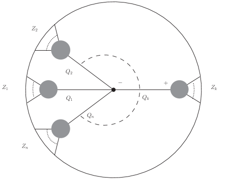
Figure 3: A vertex with all off-shell legs in arbitrary Witten diagram.

III.3 General case

Let us consider the most general case of a maximal off-shell vertex in an arbitrary Witten diagram in a scalar $\phi^{n}$  theory, as in Fig. 3. Here, the off-shell leg $Q_{k}$, is connected to the set of on-shell fields in the block named $Z_{k}$ with $k=1,\ldots,n$ via many propagators and vertices. All these intermediate propagators and vertices are collectively denoted by the blob attached to $Q_{k}$. We also assume that we had already done the $Q$ integrations for all the propagators inside each blob connected to the block $Z_{k}$ and the contribution from this to the exponent in the integrand of the $s,\bar{s},{\rm and}~{}c$ integrals is labeled as $\mathcal{B}^{Z}_{k}$. We note that this quantity depends on the variables $s,\bar{s}$ associated with all the propagators in the blob of the $k_{th}$ block $Z_{k}$ and all the $t_{k}P_{k}$’s associated with the on-shell fields contained in this block, but most importantly it does not contain the variables associated with the propagator $Q_{k}$ i.e. $s_{k}$ and $\bar{s}_{k}$.

We note that Fig. 2 is a special case of Fig. 3 if the $k_{th}$ blob contains only one maximal vertex of $\phi^{n}$ theory with $(n\!-\!1)$ on-shell legs and then $\mathcal{B}^{Z}_{k}\equiv B_{k}$.

Now it is obvious that just as in the previous section, the contribution to the Mellin exponent after doing the integrations over $Q_{1}$ to $Q_{n}$ can be written as,

$$E_{Q_{n}}=\sum_{i^{\prime}}(\mathcal{D}_{i^{\prime}})^{2}+\sum^{n}_{l=1}\big{(}\bar{s}_{l}\mathcal{Y}^{Z}_{l-1}+s_{l}\mathcal{B}^{Z}_{l}\big{)}^{2},$$ (37)

where

$$\mathcal{Y}^{Z}_{n} = \sum^{n}_{i=1}{(\prod_{k=1}^{n}g_{k})\over g_{i}}s_{i}\bar{s}_{i}\mathcal{B}^{Z}_{i}$$ (38)

and $\mathcal{D}_{i^{\prime}}$ is defined as follows. Since the $Q_{1}$ to $Q_{n}$ integrations affect the form of $\mathcal{B}_{i}^{Z}$, obtained from the previous $Q$ integrations, at each step of these integrations we will get some complicated functions which we denote as $\mathcal{D}_{i^{\prime}}$. We note that these do not have any dependence on the $s$ and $\bar{s}$ variables associated with the maximal vertex and are not of any interest for the remaining calculation. The other definitions being the same as in (18). Even though, it seems that this situation is much more complicated than before we note that none of the $\mathcal{B}^{Z}_{k}$’s depend on the $s_{k}$ and $\bar{s}_{k}$’s associated with the vertex under consideration and moreover the $\mathcal{B}^{Z}_{k}$’s are also linear in the $t_{k}P_{k}\in Z_{k}$ and hence we can apply Symanzik star formula, to perform the $t_{i}$ integrals, as before by expanding the square. Now, let us focus on the second sum in (37) and since it has the same form as (19), the analysis is similar to the one in the previous section but with a few added subtleties. In particular, when applying Symanzik star formula, the contributions from the $\mathcal{B}^{Z}_{i}\cdot\mathcal{B}^{Z}_{j}$ term will be same as that of the $B_{i}\cdot B_{j}$ term before, with $i\neq j$, but the contributions from $\mathcal{B}^{Z}_{i}\cdot\mathcal{B}^{Z}_{i}$ would be different from the analogous term in the previous section.

So all of the analysis in the previous section still holds as we can isolate the integrations for this particular vertex and write the Mellin integrand as,

$$\mathcal{M}(k_{j}) = \int ds\mathcal{V}(s)\int\prod^{n}_{j=1}{ds_{j}\over s_{j}}{d\bar{s}_{j}\over\bar{s}_{j}}\,s_{j}^{h+c_{j}+a_{j}}\bar{s}^{h-c_{j}+a_{j}}_{j}g_{j}^{-b_{j}}\prod^{n}_{j=1}H_{j}(s^{2}_{j}F_{j},s),$$ (39)

where we denote $\int ds\mathcal{V}(s)$ as the integrals irrelevant to the vertex. Even though $H_{i}(s^{2}_{i}F_{i},s)$ can be a complicated function, for the $s$ and $\bar{s}$ relevant to the vertex we are interested in, they are always of the form $s^{2}_{j}F_{j}$. So we can rescale $s^{2}_{i}$ by a factor of $F_{i}$ for $i=1,2,\dots,n$, and after rescaling, $H_{i}(s^{2}_{i}F_{i},s)$ will be included in the irrelevant integral $\int ds\mathcal{V}(s)$. So at the end we arrive at the integral related to the vertex we are interested in i.e. the $\bar{s}$ dependent part

$$\mathcal{M}(k_{i})\big{|}_{\bar{s}} = \int\prod^{n}_{i=1}{d\bar{s}_{i}\over\bar{s}_{i}}\,\bar{s}^{h-c_{i}+a_{i}}_{i}g_{i}^{-b_{i}}\prod^{n}_{i=1}F^{\frac{-h+c_{i}+a_{i}}{2}}_{i},$$ (40)

which is exactly the same as the $\bar{s}$ part of the integral in (28) and hence gives the same form of the maximal off-shell vertex.

IV Flat space limit

In this section we consider the flat space limit of the Mellin space Feynman rules. We will show that these rules give rise to the usual Feynman rules for scattering amplitudes in the flat space limit. This limit can also be considered as a consistency check of the AdS Feynman rules. The flat space limit corresponds to the large $\delta_{ij}$ behavior of the Mellin amplitudes. As had been discussed in Penedones:2010ue and Fitzpatrick:2011ia , in this limit the Mellin amplitudes are related to the S-matrix in flat space by the following relation

$$M(\delta_{ij})\approx\ \int_{0}^{\infty}d\beta\,\beta^{\frac{1}{2}\sum\Delta_{i}-h-1}e^{-\beta}\,T(p_{i}\cdot p_{j}=2\beta\delta_{ij})\ ,\ \ \ \ \ \ \ \ \delta_{ij}\gg 1\ ,$$ (41)

where $T(p_{i}\cdot p_{j}=2\beta\delta_{ij})$ is the flat space S-matrix as a function of the kinematic invariants $p_{i}\cdot p_{j}$ and $\beta$ is an integration parameter. We will study the case of large $\delta_{ij}$ limit with $\Delta_{i}$ fixed. In order to confirm that the AdS Feynman rules indeed reduce to the usual flat space Feynman rules of $\phi^{n}$ theory in this limit, we only need to show that

$$\sum_{\{n_{i}\}}M(n_{1},\dots,n_{s})={(-1)^{s}\over 2^{s}}\Gamma({1\over 2}\sum\Delta_{i}-h-s),$$ (42)

where $\sum_{\{n_{i}\}}M(n_{1},\dots,n_{s})$ related to the Mellin amplitude by

$$M(\delta_{ij})\approx\sum_{\{n_{i}\}}M(n_{1},\dots,n_{s})\prod^{s}_{i=1}{1\over k^{2}_{i}},$$ (43)

where $1\over k^{2}_{i}$ is the propagator, $s$ is the number of propagators, and the summation over $\{n_{i}\}$ become clear shortly. The above equation (42) follows directly from (41) by using the definition of the flat space massless scalar scattering amplitudes.

We will use the AdS Feynman rules (4) to compute the left hand side of (41). As in the case of $\phi^{3}$ theory Fitzpatrick:2011ia , we can always start from the bulk propagators closer to the external legs in the Witten diagram and perform the sum over $\{n_{i}\}$ recursively. To do so for a general $\phi^{n}$ theory, we need the following identity, which will be proved shortly,

$$\sum^{\infty}_{n_{I_{1}},n_{I_{2}},\dots,n_{I_{m}}=0}{V^{(1)}(n_{I_{1}})V^{(1)}(n_{I_{2}})\dots V^{(1)}(n_{I_{m}})V^{(m+1)}(n_{I_{1}},n_{I_{2}},\dots,n_{I_{m}},n_{o})\over P_{n_{I_{1}}}P_{n_{I_{2}}}\dots P_{n_{I_{m}}}}$$ (44)

$$={(-1)^{m}\over 2^{m}}((m+1)-{\sum\Delta_{i}\over 2}+\Delta_{n_{o}})_{n_{o}}\Gamma({\sum\Delta_{i}\over 2}-h-m),$$

where $P_{n}\equiv-2n!\Gamma(1+\Delta_{n}+n-h)$, and $V^{(1)}(n_{I})$ denotes the vertex with one off-shell leg where this leg is labeled as $n_{I}$, and we follow a similar logic to define $V^{(m+1)}(n_{I_{1}},n_{I_{2}},\dots,n_{I_{m}},n_{o})$, which denotes the vertex with $(m+1)$ off-shell legs. Finally, the summation in $\sum\Delta_{i}$ indicates the sum over all the external on-shell legs. The identity (44) can be proved by performing the summation in the following order: first we sum over $l_{1}$, the summation variable in the Lauricella function $F_{A}^{(n)}$ then the corresponding $n_{I_{1}}$, next we do the sum over $l_{2}$ then $n_{I_{2}}$ and so on. At each step of the sum we can apply the identity,

$$\sum^{\infty}_{n=0}{(a)_{n}(b)_{n}\over n!(c)_{n}}={(c-b)_{-a}\over(c)_{-a}}.$$ (45)

We note here that $((m+1)-{\sum\Delta_{i}\over 2}+\Delta_{n_{o}})_{n_{o}}$ in (44) has the same dependence on $n_{o}$ as $V^{(1)}(n)$ does. So the summation on $n_{o}$ in a general Witten diagram can be done by applying the above identities again. At the end of the day, we will be left with a sum involving only factors of the form of $V^{(1)}(n)$. It can be shown that the answer for the final sum of any Witten diagram is indeed given as Eq. (42).

Appendix A Useful integrals

Here we list some formulas, which have been extensively used in this paper. For more details about these formulas, see Symanzik:1972wj ; Penedones:2010ue .

$X$ integral formula

$$\int_{0}^{+\infty}\prod_{i}\left(\frac{\mathrm{d}t_{i}}{t_{i}}t^{\alpha_{i}}\right)\int_{\mbox{\tiny$AdS$}}\mathrm{d}X\,e^{2T\cdot X}=\pi^{h}\Gamma\left(\frac{\sum_{i}\alpha_{i}-2h}{2}\right)\int_{0}^{+\infty}\prod_{i}\left(\frac{\mathrm{d}t_{i}}{t_{i}}t^{\alpha_{i}}\right)e^{T^{2}},$$ (46)

where $T=\sum_{i}t_{i}P_{i}$.

$Q_{i}$ integral formula

$$\int_{0}^{+\infty}\frac{\mathrm{d}s}{s}\frac{\mathrm{d}\bar{s}}{\bar{s}}s^{h+c}s^{h-c}\,\int_{\partial\mbox{\tiny$AdS$}}\mathrm{d}Q\,e^{2T\cdot Q}=2\pi^{h}\int_{0}^{+\infty}\frac{\mathrm{d}s}{s}\frac{\mathrm{d}\bar{s}}{\bar{s}}s^{h+c}s^{h-c}e^{T^{2}},$$ (47)

where $T=(sX+\bar{s}Y)$.

$t$ integral formula

This is also called the Symanzik star integration formula where we consider a set of $n$ points in Euclidean space $x_{i}$ and their differences $x_{i}-x_{j}$. In the embedding formalism we have $P_{ij}\equiv-2P_{i}\cdot P_{j}=(x_{i}-x_{j})^{2}$. Then Symanzik’s formula is:

$$\int_{0}^{+\infty}\!\!\left(\prod_{i=1}^{n}\frac{\mathrm{d}t_{i}}{t_{i}}t^{\Delta_{i}}\right)e^{-(\sum\limits_{1\leq i<j\leq n}t_{i}t_{j}\,P_{ij})}=\frac{\pi^{h}/2}{(2\pi i)^{\frac{1}{2}n(n-3)}}\int\mathrm{d}\delta_{ij}\!\prod_{1\leq i<j\leq n}\!\!\Gamma(\delta_{ij})\,(P_{ij})^{-\delta_{ij}}$$ (48)

where the integration is over $n(n-3)/2$ variables and the integration paths are chosen parallel to the imaginary axis, with real parts such that the real parts of the arguments of the gamma functions are positive.

Appendix B Example: $9$-points in $\phi^{3}$ theory

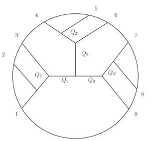
Figure 4: A vertex with all off-shell legs in $9$-point amplitude in $\phi^{3}$ theory

In order to illustrate the general strategy of isolating the maximal vertex in any arbitrary Witten diagram, as discussed in section $3.3$, here we will study a specific example, that of a $9$-point Witten diagram in $\phi^{3}$ theory and we will write down the results as a special case of (39) and (40). We have the $Q$ variables labeled as $Q_{1^{\prime}},Q_{2^{\prime}},Q_{3^{\prime}},Q_{1},Q_{2},Q_{3}$ and then we will integrate them out in that particular order. We note here that only the variables $Q_{1},Q_{2},Q_{3}$ are relevant for the vertex under consideration. After doing all the $Q$ integrals we will get the exponent as before given by (37),

$$E_{Q_{3}}=\sum_{i=1}^{3}(\mathcal{D}_{i^{\prime}})^{2}+\sum^{3}_{l=1}\big{(}\bar{s}_{l}\mathcal{Y}^{Z}_{l-1}+s_{l}\mathcal{B}^{Z}_{l}\big{)}^{2},$$ (49)

where the term in the first bracket is given by

$$\mathcal{D}_{1^{\prime}} = P_{3}t_{3}\bar{s}_{1^{\prime}}+s_{1^{\prime}}\left(P_{1}t_{1}+P_{2}t_{2}\right),$$

$$\mathcal{D}_{2^{\prime}} = P_{6}t_{6}\bar{s}_{2^{\prime}}+s_{2^{\prime}}\left(P_{4}t_{4}+P_{5}t_{5}\right),$$

$$\mathcal{D}_{3^{\prime}} = P_{9}t_{9}\bar{s}_{3^{\prime}}+s_{3^{\prime}}\left(P_{7}t_{7}+P_{8}t_{8}\right),$$ (50)

and these terms do not contain any of the variables relevant to the vertex we are interested in and hence we will not consider them further. Now let us focus on the term inside the second bracket where the relevant functions $\mathcal{B}^{Z}$ and $\mathcal{Y}^{Z}$, defined by (38), are given by,

$$\mathcal{B}^{Z}_{1} = \mathcal{D}_{1^{\prime}}\bar{s}_{1^{\prime}}+P_{3}t_{3},$$

$$\mathcal{B}^{Z}_{2} = \mathcal{D}_{2^{\prime}}\bar{s}_{2^{\prime}}+P_{6}t_{6},$$

$$\mathcal{B}^{Z}_{3} = \mathcal{D}_{3^{\prime}}\bar{s}_{3^{\prime}}+P_{9}t_{9}$$ (51)

and

$$\mathcal{Y}^{Z}_{0} = 0,$$

$$\mathcal{Y}^{Z}_{1} = s_{1}\mathcal{B}^{Z}_{1}\bar{s}_{1},$$

$$\mathcal{Y}^{Z}_{2} = s_{2}\mathcal{B}^{Z}_{2}\left(\bar{s}_{1}^{2}+1\right)\bar{s}_{2}+s_{1}\mathcal{B}^{Z}_{1}\bar{s}_{1}\left(\left(\bar{s}_{1}^{2}+1\right)\bar{s}_{2}^{2}+1\right).$$ (52)

The next step is to expand the second term of $E_{Q_{3}}$ like before and after doing all the $t_{i}$ integrals we get the form of the integrand as in (39),

$$\mathcal{M}(k_{j}) = \int ds\mathcal{V}(s)\int\prod^{3}_{j=1}{ds_{j}\over s_{j}}{d\bar{s}_{j}\over\bar{s}_{j}}\,s_{j}^{h+c_{j}+a_{j}}\bar{s}^{h-c_{j}+a_{j}}_{j}g_{j}^{-b_{j}}\prod^{3}_{j=1}H_{j}(s^{2}_{j}F_{j},s),$$ (53)

where $g$ and $F$ are defined by (18) and (21) and $a_{j},b_{j}$ are defined by (25) and (26) respectively. Moreover, the part which is irrelevant to the maximal vertex is given by

$$\mathcal{V}(s) = \prod^{3^{\prime}}_{j=1^{\prime}}{ds_{j}\over s_{j}}s_{j}^{h+c_{j}+a^{\prime}_{j}}\bar{s}_{j}^{h-c_{j}+a^{\prime}_{j}}\left(\bar{s}_{1^{\prime}}^{2}+1\right){}^{-k_{3}\left(k_{1}+k_{2}+k_{3}\right)}$$ (54)

$$\times \left(\bar{s}_{2^{\prime}}^{2}+1\right){}^{-k_{6}\left(k_{4}+k_{5}+k_{6}\right)}\left(\bar{s}_{3^{\prime}}^{2}+1\right){}^{-k_{9}\left(k_{7}+k_{8}+k_{9}\right)},$$

where,

$$a^{\prime}_{1^{\prime}} = -(k_{1}+k_{2})^{2},$$

$$a^{\prime}_{2^{\prime}} = -(k_{4}+k_{5})^{2},$$

$$a^{\prime}_{3^{\prime}} = -(k_{7}+k_{8})^{2}.$$ (55)

The complicated $H$ function which would eventually give the terms relevant for the vertex, is given by,

$$H_{1}(s^{2}_{1}F_{1},s) = \left(F_{1}s_{1}^{2}\left(\bar{s}_{1^{\prime}}^{2}+1\right)+1\right){}^{\left(k_{1}+k_{2}\right)k_{3}}\left(s_{1^{\prime}}^{2}\left(F_{1}s_{1}^{2}\bar{s}_{1^{\prime}}^{2}+1\right)+1\right){}^{k_{1}k_{2}},$$

$$H_{2}(s^{2}_{2}F_{2},s) = \left(F_{2}s_{2}^{2}\left(\bar{s}_{2^{\prime}}^{2}+1\right)+1\right){}^{\left(k_{4}+k_{5}\right)k_{6}}\left(s_{2^{\prime}}^{2}\left(F_{2}s_{2}^{2}\bar{s}_{2^{\prime}}^{2}+1\right)+1\right){}^{k_{4}k_{5}},$$

$$H_{3}(s^{2}_{3}F_{3},s) = \left(F_{3}s_{3}^{2}\left(\bar{s}_{3^{\prime}}^{2}+1\right)+1\right){}^{\left(k_{7}+k_{8}\right)k_{9}}\left(s_{3^{\prime}}^{2}\left(F_{3}s_{3}^{2}\bar{s}_{3^{\prime}}^{2}+1\right)+1\right){}^{k_{7}k_{8}}.$$ (56)

Now, as before, we can use the the transformation

$$s_{i}^{2}\rightarrow\frac{s_{i}^{2}}{F_{i}}$$ (57)

and we will get the required form of the $\bar{s}$ integral part as in (40), to be

$$\mathcal{M}(k_{i})\big{|}_{\bar{s}} = \int\prod^{3}_{i=1}{d\bar{s}_{i}\over\bar{s}_{i}}\,\bar{s}^{h-c_{i}+a_{i}}_{i}g_{i}^{-b_{i}}F^{\frac{-h+c_{i}+a_{i}}{2}}_{i}.$$ (58)

From (56) we also see that after the rescaling of $s^{2}_{i}$’s we are left with a term of the form ,

$$\mathcal{V}^{\prime}(s) = \left(s_{1}^{2}\left(\bar{s}_{1^{\prime}}^{2}+1\right)+1\right){}^{\left(k_{1}+k_{2}\right)k_{3}}\left(s_{1^{\prime}}^{2}\left(s_{1}^{2}\bar{s}_{1^{\prime}}^{2}+1\right)+1\right){}^{k_{1}k_{2}}$$ (59)

$$\times \left(s_{2}^{2}\left(\bar{s}_{2^{\prime}}^{2}+1\right)+1\right){}^{\left(k_{4}+k_{5}\right)k_{6}}\left(s_{2^{\prime}}^{2}\left(s_{2}^{2}\bar{s}_{2^{\prime}}^{2}+1\right)+1\right){}^{k_{4}k_{5}}$$

$$\times \left(s_{3}^{2}\left(\bar{s}_{3^{\prime}}^{2}+1\right)+1\right){}^{\left(k_{7}+k_{8}\right)k_{9}}\left(s_{3^{\prime}}^{2}\left(s_{3}^{2}\bar{s}_{3^{\prime}}^{2}+1\right)+1\right){}^{k_{7}k_{8}},$$

which we note is independent of the $\bar{s}$ variables related to the maximal vertex and hence irrelevant.

References

- (1) J. M. Maldacena, “The Large N limit of superconformal field theories and supergravity,” Adv.Theor.Math.Phys. 2 (1998) 231–252, arXiv:hep-th/9711200 [hep-th].
- (2) E. Witten, “Anti-de Sitter space and holography,” Adv.Theor.Math.Phys. 2 (1998) 253–291, arXiv:hep-th/9802150 [hep-th].
- (3) S. Gubser, I. R. Klebanov, and A. M. Polyakov, “Gauge theory correlators from noncritical string theory,” Phys.Lett. B428 (1998) 105–114, arXiv:hep-th/9802109 [hep-th].
- (4) H. Liu and A. A. Tseytlin, “On four-point functions in the CFT/AdS correspondence,”Phys. Rev. D59 (1999) 086002, arXiv:hep-th/9807097.
- (5) H. Liu, “Scattering in anti-de Sitter space and operator product expansion,” Phys. Rev. D 60, 106005 (1999) arXiv:hep-th/9811152.
- (6) E. D’Hoker and D. Z. Freedman, “General scalar exchange in AdS(d+1),” Nucl. Phys. B550 (1999) 261–288, arXiv:hep-th/9811257.
- (7) D. Z. Freedman, S. D. Mathur, A. Matusis, and L. Rastelli, “Comments on 4-point functions in the CFT/AdS correspondence,” Phys. Lett. B452 (1999) 61–68, arXiv:hep-th/9808006.
- (8) D. Z. Freedman, S. D. Mathur, A. Matusis, and L. Rastelli, “Correlation functions in the CFT()/AdS() correspondence,” Nucl. Phys. B546 (1999) 96–118, arXiv:hep-th/9804058.
- (9) E. D’Hoker, D. Z. Freedman, S. D. Mathur, A. Matusis, and L. Rastelli, “Graviton exchange and complete 4-point functions in the AdS/CFT correspondence,” Nucl. Phys. B562 (1999) 353–394, arXiv:hep-th/9903196.
- (10) G. Arutyunov and S. Frolov, “Four-point functions of lowest weight CPOs in N = 4 SYM(4) in supergravity approximation,” Phys. Rev. D62 (2000) 064016, arXiv:hep-th/0002170.
- (11) G. Arutyunov, F. A. Dolan, H. Osborn, and E. Sokatchev, “Correlation functions and massive Kaluza-Klein modes in the AdS/CFT correspondence,” Nucl. Phys. B665 (2003) 273–324, arXiv:hep-th/0212116.
- (12) G. Arutyunov and E. Sokatchev, “On a large N degeneracy in N = 4 SYM and the AdS/CFT correspondence,” Nucl. Phys. B663 (2003) 163–196, arXiv:hep-th/0301058.
- (13) L. Berdichevsky and P. Naaijkens, “Four-point functions of different-weight operators in the AdS/CFT correspondence,” JHEP 01 (2008) 071, arXiv:0709.1365 [hep-th].
- (14) L. I. Uruchurtu, “Four-point correlators with higher weight superconformal primaries in the AdS/CFT Correspondence,” JHEP 03 (2009) 133, arXiv:0811.2320 [hep-th].
- (15) E. I. Buchbinder and A. A. Tseytlin, “On semiclassical approximation for correlators of closed string vertex operators in AdS/CFT,” JHEP 08 (2010) 057, arXiv:1005.4516 [hep-th].
- (16) L. I. Uruchurtu, “Next-next-to-extremal Four Point Functions of N=4 1/2 BPS Operators in the AdS/CFT Correspondence,” arXiv:1106.0630 [hep-th].
- (17) F. A. Dolan, M. Nirschl, and H. Osborn, “Conjectures for large N N = 4 superconformal chiral primary four point functions,” Nucl. Phys. B749 (2006) 109–152, arXiv:hep-th/0601148.
- (18) E. D’Hoker, D. Z. Freedman, and L. Rastelli, “AdS/CFT 4-point functions: How to succeed at z-integrals without really trying,” Nucl. Phys. B562 (1999) 395–411, arXiv:hep-th/9905049.
- (19) S. Raju, “BCFW for Witten Diagrams,” Phys.Rev.Lett. 106 (2011) 091601, arXiv:1011.0780 [hep-th].
- (20) S. Raju, “Recursion Relations for AdS/CFT Correlators,” Phys. Rev. D83 (2011) 126002, arXiv:1102.4724 [hep-th].
- (21) G. Mack, “D-independent representation of Conformal Field Theories in D dimensions via transformation to auxiliary Dual Resonance Models. Scalar amplitudes,” arXiv:0907.2407 [hep-th].
- (22) G. Mack, “D-dimensional Conformal Field Theories with anomalous dimensions as Dual Resonance Models,” arXiv:0909.1024 [hep-th].
- (23) J. Penedones, “Writing CFT correlation functions as AdS scattering amplitudes,” JHEP 1103, 025 (2011) arXiv:1011.1485 [hep-th].
- (24) M. F. Paulos, “Towards Feynman rules for Mellin amplitudes,” arXiv:1107.1504 [hep-th].
- (25) A. L. Fitzpatrick, J. Kaplan, J. Penedones, S. Raju and B. C. van Rees, “A Natural Language for AdS/CFT Correlators,” arXiv:1107.1499 [hep-th].
- (26) M. S. Costa, J. Penedones, D. Poland and S. Rychkov, “Spinning Conformal Correlators,” JHEP 1111, 071 (2011) arXiv:1107.3554 [hep-th].
- (27) M. S. Costa, J. Penedones, D. Poland and S. Rychkov, “Spinning Conformal Blocks,” arXiv:1109.6321 [hep-th].
- (28) I. Balitsky, “Mellin representation of the graviton bulk-to-bulk propagator in AdS,” Phys. Rev. D 83, 087901 (2011) arXiv:1102.0577 [hep-th]].
- (29) L. Susskind, “Holography in the flat space limit,” arXiv:hep-th/9901079.
- (30) J. Polchinski, “S-matrices from AdS spacetime,” arXiv:hep-th/9901076.
- (31) M. Gary, S. B. Giddings, and J. Penedones, “Local bulk S-matrix elements and CFT singularities,” Phys. Rev. D80 (2009) 085005, arXiv:0903.4437 [hep-th].
- (32) I. Heemskerk, J. Penedones, J. Polchinski, and J. Sully, “Holography from Conformal Field Theory,” JHEP 10 (2009) 079, arXiv:0907.0151 [hep-th].
- (33) A. L. Fitzpatrick, E. Katz, D. Poland, and D. Simmons-Duffin, “Effective Conformal Theory and the Flat-Space Limit of AdS,” arXiv:1007.2412 [hep-th].
- (34) T. Okuda and J. Penedones, “String scattering in flat space and a scaling limit of Yang-Mills correlators,” arXiv:1002.2641 [hep-th].
- (35) A. Fitzpatrick and J. Kaplan, “Scattering States in AdS/CFT,” arXiv:1104.2597 [hep-th].
- (36) M. Gary and S. B. Giddings, “The flat space S-matrix from the AdS/CFT correspondence?,” Phys. Rev. D80 (2009) 046008, arXiv:0904.3544 [hep-th].
- (37) S. B. Giddings, “Flat-space scattering and bulk locality in the AdS/CFT correspondence,” Phys. Rev. D61 (2000) 106008, arXiv:hep-th/9907129.
- (38) M. Gary and S. B. Giddings, “Constraints on a fine-grained AdS/CFT correspondence,” arXiv:1106.3553 [hep-th].
- (39) K. Symanzik, “On Calculations in conformal invariant field theories,” Lett. Nuovo Cim. 3, 734 (1972).
- (40) A. Fitzpatrick and J. Kaplan, “Analyticity and the Holographic S-Matrix,” arXiv:1111.6972v1 [hep-th].