Abstract

We briefly recall the main physical features of the parton distributions in the quantum statistical picture of the nucleon. Some predictions from a next-to-leading order QCD analysis are successfully compared to recent unpolarized and polarized experimental results. We will discuss the extension to the transverse momentum dependence of the parton distributions and its relevance for semiinclusive deep inelastic scattering. Finally, we will present some new positivity constraints for spin observables and their implications for parton distributions.

Keywords: Polarized electroproduction, proton spin structure

PACS: 12.40.Ee, 13.60.Hb, 13.88.+e,14.65.Bt

1 A short review on the statistical approach

Let us first recall some of the basic ingredients for building up the parton distribution functions (PDF) in the statistical approach, as oppose to the standard polynomial type parametrizations, based on Regge theory at low $x$ and counting rules at large $x$. The fermion distributions are expressed by the sum of two terms [1], the first one, a quasi Fermi-Dirac function, for a given helicity and flavor, and the second one, a flavor and helicity independent diffractive contribution equal for light quarks. So we have, at the input energy scale $Q_{0}^{2}=4\mbox{GeV}^{2}$,

$$xq^{h}(x,Q^{2}_{0})=\frac{AX^{h}_{0q}x^{b}}{\exp[(x-X^{h}_{0q})/\bar{x}]+1}+\frac{\tilde{A}x^{\tilde{b}}}{\exp(x/\bar{x})+1}~{},$$ (1)

$$x\bar{q}^{h}(x,Q^{2}_{0})=\frac{{\bar{A}}(X^{-h}_{0q})^{-1}x^{2b}}{\exp[(x+X^{-h}_{0q})/\bar{x}]+1}+\frac{\tilde{A}x^{\tilde{b}}}{\exp(x/\bar{x})+1}~{}.$$ (2)

Notice the change of sign of the potentials and helicity for the antiquarks. The parameter $\bar{x}$ plays the role of a universal temperature and $X^{\pm}_{0q}$ are the two thermodynamical potentials of the quark $q$, with helicity $h=\pm$. It is important to remark that the diffractive contribution occurs only in the unpolarized distributions $q(x)=q_{+}(x)+q_{-}(x)$ and it is absent in the valence $q_{v}(x)=q(x)-\bar{q}(x)$ and in the helicity distributions $\Delta q(x)=q_{+}(x)-q_{-}(x)$ (similarly for antiquarks). The eight free parameters in Eqs. (1,2) were determined at the input scale from the comparison with a selected set of very precise unpolarized and polarized Deep Inelastic Scattering (DIS) data [1]. They have the following values

$$\bar{x}=0.09907,~{}b=0.40962,~{}\tilde{b}=-0.25347,~{}\tilde{A}=0.08318,$$ (3)

$$X^{+}_{0u}=0.46128,~{}X^{-}_{0u}=0.29766,~{}X^{-}_{0d}=0.30174,~{}X^{+}_{0d}=0.22775~{}.$$ (4)

For the gluons we consider the black-body inspired expression

$$xG(x,Q^{2}_{0})=\frac{A_{G}x^{b_{G}}}{\exp(x/\bar{x})-1}~{},$$ (5)

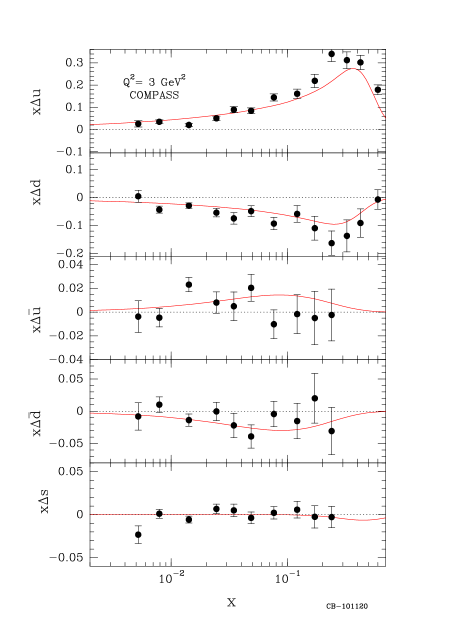
Figure 2: Left : Quark and antiquark helicity distributions as a function of $x$ for $Q^{2}=3\mbox{GeV}^{2}$. Data from COMPASS [10]. The curves are predictions from the statistical approach. Right : Ratios $(\Delta u+\Delta\bar{u})/(u+\bar{u})$ and $(\Delta d+\Delta\bar{d})/(d+\bar{d})$ as a function of $x$. Data from Hermes for $Q^{2}=2.5\mbox{GeV}^{2}$ [11] and a JLab Hall A experiment [12]. The curves are predictions from the statistical approach

a quasi Bose-Einstein function, with $b_{G}=0.90$, the only free parameter , since $A_{G}=20.53$ is determined by the momentum sum rule. We also assume that, at the input energy scale, the polarized gluon distribution vanishes, so $x\Delta G(x,Q^{2}_{0})=0$. For the strange quark distributions, the simple choice made in Ref. [1] was greatly improved in Ref. [2]. More recently, new tests against experimental (unpolarized and polarized) data turned out to be very satisfactory, in particular in hadronic collisions, as reported in Refs. [3, 4].
An interesting point concerns the behavior of the ratio $d(x)/u(x)$, which depends on the mathematical properties of the ratio of two Fermi-Dirac factors, outside the region dominated by the diffractive contribution. So for $x>0.1$, this ratio is expected to decrease faster for $X_{0d}^{+}-\bar{x}<x<X_{0u}^{+}+\bar{x}$ and then above, for $x>0.6$, it flattens out.
This change of slope is clearly visible in Fig. 1 (Left), with a very little $Q^{2}$ dependence. Note that our prediction for the large $x$ behavior, differs from most of the current literature, namely $d(x)/u(x)\to 0$ for $x\to 1$, but we find $d(x)/u(x)\to 0.16$ near the value $1/5$, a prediction originally formulated in Ref. [5]. This is a very challenging question, since the very high-$x$ region remains poorly known. To continue our tests of the unpolarized parton distributions, we must come back to the important question of the flavor asymmetry of the light antiquarks. Our determination of $\bar{u}(x,Q^{2})$ and $\bar{d}(x,Q^{2})$ is perfectly consistent with the violation of the Gottfried sum rule, for which we found the value $I_{G}=0.2493$ for $Q^{2}=4\mbox{GeV}^{2}$. Nevertheless there remains an open problem with the $x$ distribution of the ratio $\bar{d}(x)/\bar{u}(x)$ for $x\geq 0.2$. According to the Pauli principle, this ratio is expected to remain above 1 for any value of $x$. However, the E866/NuSea Collaboration [6] has released the final results corresponding to the analysis of their full data set of Drell-Yan yields from an 800 GeV/c proton beam on hydrogen and deuterium targets and they obtain the ratio, for $Q^{2}=54\mbox{GeV}^{2}$, $\bar{d}(x)/\bar{u}(x)$ shown in Fig. 1 (Right). Although the errors are rather large in the high-$x$ region, the statistical approach disagrees with the trend of the data. Clearly by increasing the number of free parameters, it is possible to build up a scenario which leads to the drop off of this ratio for $x\geq 0.2$. For example this was achieved in Ref. [7], as shown by the dashed curve in Fig. 1 (Right). There is no such freedom in the statistical approach, since quark and antiquark distributions are strongly related. On the experimental side, there are now new opportunities for extending the $\bar{d}(x)/\bar{u}(x)$ measurement to larger $x$ up to $x=0.7$, with the upcoming E906 experiment at the 120 GeV Main Injector at Fermilab [8] and a proposed experiment at the new 30-50 GeV proton accelerator at J-PARC [9].
Analogous considerations can be made for the corresponding helicity distributions, whose most recent determinations are shown in Fig. 2 (Left). By using a similar argument as above, the ratio $\Delta u(x)/u(x)$ is predicted to have a rather fast increase in the $x$ range $(X^{-}_{0u}-\bar{x},X^{+}_{0u}+\bar{x})$ and a smoother behaviour above, while $\Delta d(x)/d(x)$, which is negative, has a fast decrease in the $x$ range $(X^{+}_{0d}-\bar{x},X^{-}_{0d}+\bar{x})$ and a smooth one above. This is exactly the trends displayed in Fig. 2 (Right) and our predictions are in perfect agreement with the accurate high-$x$ data. We note the behavior near $x=1$, another typical property of the statistical approach, is also at variance with predictions of the current literature. The fact that $\Delta u(x)$ is more concentrated in the higher $x$ region than $\Delta d(x)$, accounts for the change of sign of $g^{n}_{1}(x)$, which becomes positive for $x>0.5$, as first observed at Jefferson Lab [12].
Concerning the light antiquark helicity distributions, the statistical approach imposes a strong relationship to the corresponding quark helicity distributions. In particular, it predicts $\Delta\bar{u}(x)>0$ and $\Delta\bar{d}(x)<0$, with almost the same magnitude, in contrast with the simplifying assumption $\Delta\bar{u}(x)=\Delta\bar{d}(x)$, often adopted in the literature. According to the COMPASS experiment at CERN [13], $\Delta\bar{u}(x)+\Delta\bar{d}(x)\simeq 0$, in agreement with our prediction.

2 The TMD extension

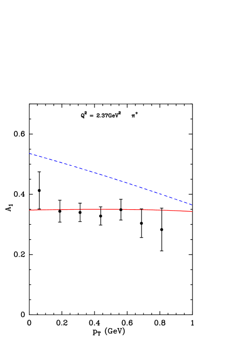
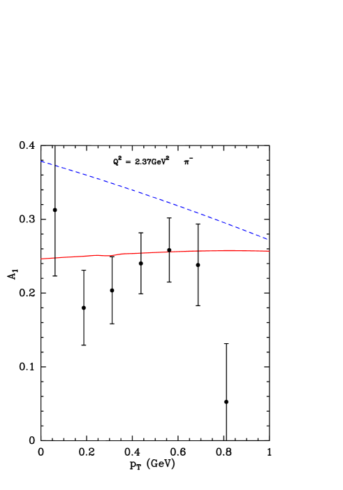
Figure 3: Left : The double longitudinal-spin asymmetry $A_{1}$ for $\pi^{+}$ production on a proton target, versus the $\pi^{+}$ momentum $p_{T}$, compared to the JLab data Ref. [17]. The solid lines are the results from the TMD statistical distributions [15] and the dashed lines correspond to the relativistic covariant distributions [16] Right : Same for $\pi^{-}$.

We now turn to another important aspect of the statistical PDF and very briefly discuss a new version of the extension to the transverse momentum dependence (TMD). In Eqs. (1,2) the multiplicative factors $X^{h}_{0q}$ and $(X^{-h}_{0q})^{-1}$ in the numerators of the non-diffractive parts of $q$’s and $\bar{q}$’s distributions, imply a modification of the quantum statistical form, we were led to propose in order to agree with experimental data. The presence of these multiplicative factors was justified in our earlier attempt to generate the TMD [14], but it was not properly done and a considerable improvement was achieved recently [15]. We have introduced some thermodynamical potentials $Y^{h}_{0q}$, associated to the quark transverse momentum $k_{T}$, and related to $X^{h}_{0q}$ by the simple relation $\mbox{ln}(1+\exp[Y^{h}_{0q}])=kX^{h}_{0q}$. We were led to choose $k=3.05$ and this method involves another parameter $\mu^{2}$, which plays the role of the temperature for the transverse degrees of freedom and whose value was determined by the transverse energy sum rule. We have calculated the $p_{T}$ dependence of semiinclusive DIS cross sections and double longitudinal spin asymmetries, taking into account the effects of the Melosh-Wigner rotation, for $\pi^{\pm}$ production by using this set of TMD statistical parton distributions and another set coming from the relativistic covariant approach [16]. Both sets do not satisfy the usual factorization assumption of the dependence in $x$ and $k_{T}$ and they lead to different results, which can be compared to recent experimental data from CLAS at JLab, as shown on Figs. 3.

3 Positivity bounds

Spin observables for any particle reaction, contain some unique information which allow a deeper understanding of the nature of the underlying dynamics and this is very usefull to check the validity of theoretical assumptions. We emphasize the relevance of positivity in spin physics, which puts non-trivial model independent constraints on spin observables. If one, two or several observables are measured, the constraints can help to decide which new observable will provide the best improvement of knowledge. Different methods can be used to establish these constraints and they have been presented together with many interesting cases in a review article [18]. For lack of space, here we will only briefly discuss some new results obtained very recently [19, 20].
Let us consider the inclusive reaction of the type $A(\mbox{spin 1/2})+B(\mbox{spin 1/2})\to C+X$, where both initial spin $1/2$ particles can be in any possible directions and no polarization is observed in the final state. The spin-dependent corresponding cross section $\sigma\left(P_{a},P_{b}\right)={\rm Tr}\left(M\rho\right)$, can be defined through the $4\times 4$ cross section matrix $M$ and the spin density matrix $\rho$, where $P_{a}$, $P_{b}$ are the spin unit vectors of $A$ and $B$, $\rho=\rho_{a}\otimes\rho_{b}$ is the spin density matrix with $\rho_{a}=(I_{2}+P_{a}\cdot\vec{\sigma}_{a})/2$, and similar for $\rho_{b}$. Here $I_{2}$ is the $2\times 2$ unit matrix, and $\sigma=(\sigma_{x},\sigma_{y},\sigma_{z})$ stands for the $2\times 2$ Pauli matrices. $M$ can be parametrized in terms of 8 parity-conserving asymmetries and 8 parity-violating asymmetries. The crucial point is that $M$ is a Hermitian and positive matrix and this allows to derive some positivity conditions. Since one of the necessary conditions for a Hermitian matrix to be positive definite is that all the diagonal matrix elements has to be positive $M_{ii}\geq 0$, we thus derive $1\pm A_{NN}\geq\left|A_{aN}\pm A_{bN}\right|$, valid in full generality, for both parity-conserving and parity-violating processes, where $A_{N}$ denotes the single transverse spin asymmetry and $A_{NN}$ the double transverse spin asymmetry. In the case $p^{\uparrow}+p^{\uparrow}\to C+X$ where the initial particles are identical, we have $A_{aN}(y)=-A_{bN}(-y)$. Using this relation , one obtains, $1\pm A_{NN}(y)\geq\left|A_{N}(y)\mp A_{N}(-y)\right|$. This is an interesting result which, can be used, in principle, with available data on $A_{N}$ for $\pi^{\pm}$, $K^{\pm}$, $\pi^{0}$, $\eta$ production, to put some non trivial contraints on $A_{NN}(y)$.
Let us now study the implications of the above relation for the parity-violating process $p^{\uparrow}+p^{\uparrow}\to W^{\pm}+X$. Since $A_{NN}\approx 0$, to a very good approximation, it reduces to $1/2\geq|A_{N}(y=0)|$, to be compared with the usual trivial bound $1\geq|A_{N}(y=0)|$.

The TMD quark distribution in a transversely polarized hadron can be expanded as $f_{q/h^{\uparrow}}(x,\mathbf{k}_{\perp},\vec{S})\equiv f_{q/h}(x,k_{\perp})+\frac{1}{2}\Delta^{N}f_{q/h^{\uparrow}}(x,k_{\perp})\,\vec{S}\cdot\left(\hat{p}\times\hat{\mathbf{k}}_{\perp}\right)$, where $\hat{p}$ and $\hat{\mathbf{k}}_{\perp}$ are the unit vectors of $\vec{p}$ and $\mathbf{k}_{\perp}$, respectively. $f_{q/h}(x,k_{\perp})$ is the spin-averaged TMD distribution, and $\Delta^{N}f_{q/h^{\uparrow}}(x,k_{\perp})$ is the Sivers function. There is a trivial positivity bound for the Sivers functions which reads $|\Delta^{N}f_{q/h^{\uparrow}}(x,k_{\perp})|\leq 2f_{q/h}(x,k_{\perp})$. Since $A_{N}$ is directly expressed in terms of $\Delta^{N}f_{q/h^{\uparrow}}(x,k_{\perp})$, this trivial bound can be improved as shown in Ref. [20].
In the helicity basis it is easy to obtain the explicit form of $M$ and now from $M_{ii}\geq 0$, we have $1\pm A_{LL}(y)\geq|A_{aL}(y)\pm A_{bL}(y)|$, where $A_{L}$ denotes the single helicity asymmetry and $A_{LL}$ the double double asymmetry. It is important to note that for identical initial particles scattering, one has $A_{aL}(y)=A_{bL}(-y)$, so one gets $1\pm A_{LL}(y)\geq|A_{L}(y)\pm A_{L}(-y)|$. These bounds should be tested in RHIC experiments for $W^{\pm}$ or $Z^{0}$ production in longitudinal $pp$ collisions, $\vec{p}\vec{p}\to W^{\pm}/Z^{0}+X$. In perturbative QCD formalism, at leading-order and restricting to only up and down quarks, one has simple expressions for the single and double helicity asymmetries, involving only quark helicity distributions. The statistical PDF satisfy the positivity bound. Finally at $y=0$, since $A_{LL}(0)$ is expected to be very small, the bound implies $A_{L}(0)\leq 1/2$, a remarquable simple result which must be satisfied by future experimental data.

Acknowledgments
I am grateful to the organizers of DSPIN2011 for their warm hospitality at JINR and for their invitation to present this talk. My special thanks go to Prof. A.V. Efremov for providing a full financial support and for making, once more, this meeting so successful.

Figure 1: Left : The ratio $d(x)/u(x)$ as function of $x$ for $Q^{2}=4\mbox{GeV}^{2}$ (solid line) and $Q^{2}=100\mbox{GeV}^{2}$ (dashed-dotted line). Right : Comparison of the data on $\bar{d}/\bar{u}(x,Q^{2})$ from E866/NuSea at $Q^{2}=54\mbox{GeV}^{2}$ [6], with the prediction of the statistical model (solid curve) and the set 1 of the parametrization proposed in Ref. [7] (dashed curve).

References

-
[1]
C. Bourrely, F. Buccella and J. Soffer, Euro. Phys. J. C23, (2002) 487.
For a practical use of these PDF, we refer the reader to the following web site:
www.cpt.univ-mrs.fr/ bourrely/research/bbs-dir/bbs.html. - [2] C. Bourrely, F. Buccella and J. Soffer, Phys. Lett. B648, (2007) 39.
- [3] C. Bourrely, F. Buccella and J. Soffer, Mod. Phys. Letters A18, (2003) 771 ; Euro. Phys. J. C41, (2005) 327.
- [4] C. Bourrely, F. Buccella and J. Soffer, Euro. Phys. J. C41, (2005) 327.
- [5] G.R. Farrar and D.R. Jackson, Phys. Rev. Lett. 35, (1975) 1416.
- [6] R.S. Towell et al., [FNAL E866/Nusea Collaboration], Phys. Rev. D64, (2001) 052002.
- [7] A. Daleo, C.A. García Canal, G.A. Navarro and R. Sassot, Int. J. Mod. Phys. A17, (2002) 269.
- [8] D.F. Geesaman et al., [E906 Collaboration], FNAL Proposal E906, April 1, 2001.
- [9] J.C.. Peng et al., hep-ph/0007341.
- [10] M. Alekseev et al., [COMPASS Collaboration], Phys. Lett. B693, (2010) 227.
- [11] K. Ackerstaff et al., [Hermes Collaboration], Phys. Lett. B464, (1999) 123.
- [12] X. Zheng et al., [Jefferson Lab Hall A Collaboration], Phys. Rev. C70, (2004) 065207.
- [13] M. Alekseev et al., [COMPASS Collaboration], Phys. Lett. B660, (2008) 458.
- [14] C. Bourrely, F. Buccella and J. Soffer, Mod. Phys. Letters A21, (2006) 143.
- [15] C. Bourrely, F. Buccella and J. Soffer, Phys. Rev. D83, (2011) 074008.
- [16] P. Zavada, Eur. Phys. J. C52, 121 (2007) and references therein. A.V. Efremov, P. Schweitzer, O.V. Teryaev and P. Zavada, Proceedings of XIII Workshop on High Energy Spin Physics DSPIN-09, Dubna, Russia, Sept. 1-5, 2009. arXiv:0912.3380v3 [hep-ph] and references therein. See also arXiv:1008.3827v1 [hep-ph].
- [17] H. Avakian , [CLAS Collaboration], Phys. Rev. Lett. 105, (2010) 262002.
- [18] X. Artru, M. Elchikh, J.M. Richard, J. Soffer and O. Teryaev, Physics Reports 470, (2009) 1.
- [19] Zhong-Bo Kang and J. Soffer, Phys. Rev. D83, (2011) 114020.
- [20] Zhong-Bo Kang and J. Soffer, Phys. Lett B695, (2011) 275.